Remote State Estimation with Smart Sensors over Markov Fading Channels
Abstract
††W. Liu, Y. Li and B. Vucetic are with School of Electrical and Information Engineering, The University of Sydney, Australia. Emails: {wanchun.liu, yonghui.li, branka.vucetic}@sydney.edu.au. D. E. Quevedo is with the School of Electrical Engineering and Robotics, Queensland University of Technology (QUT), Brisbane, Australia. Email: daniel.quevedo@qut.edu.au. K. H. Johansson is with School of Electrical Engineering and Computer Science, KTH Royal Institute of Technology, Stockholm, Sweden. Email: kallej@kth.se.We consider a fundamental remote state estimation problem of discrete-time linear time-invariant (LTI) systems. A smart sensor forwards its local state estimate to a remote estimator over a time-correlated multi-state Markov fading channel, where the packet drop probability is time-varying and depends on the current fading channel state. We establish a necessary and sufficient condition for mean-square stability of the remote estimation error covariance in terms of the state transition matrix of the LTI system, the packet drop probabilities in different channel states, and the transition probability matrix of the Markov channel states. To derive this result, we propose a novel estimation-cycle based approach, and provide new element-wise bounds of matrix powers. The stability condition is verified by numerical results, and is shown more effective than existing sufficient conditions in the literature. We observe that the stability region in terms of the packet drop probabilities in different channel states can either be convex or non-convex depending on the transition probability matrix of the Markov channel states. Our numerical results suggest that the stability conditions for remote estimation may coincide for setups with a smart sensor and with a conventional one (which sends raw measurements to the remote estimator), though the smart sensor setup achieves a better estimation performance.
Index Terms:
Estimation, Kalman filtering, linear systems, stability, mean-square error, Markov fading channelI Introduction
I-A Motivation
In the long-term evolution of wireless applications from conventional wireless sensor networks (WSNs) to the Internet-of-Things (IoT) and the Industry 4.0, remote estimation is a key component [1, 2, 3, 4]. Driven by Moore’s Law, the accelerated development and adoption of smart sensor technology enables low-cost sensors with high computational capability [5]. Thus, in a number of remote estimation applications, it is practical to use smart sensors (e.g., with Kalman filters) to pre-estimate the dynamic states, and then send the estimated states rather than the raw measurements to the remote estimator. In the presence of communication constraints, the smart sensors provide better estimation performance than the conventional sensors that purely send raw measurement data to the remote estimator [6].
Unlike wired communications, wireless communications are unreliable and the channel status varies with time due to multipath propagation and shadowing caused by obstacles affecting the wave propagation. The transition process of the fading channel states is usually modeled as a Markov process [7, 8, 9], and different channel states lead to different packet drop probabilities of transmissions. The presence of an unreliable wireless communication channel degrades the estimation performance, and in some cases even lead to instability. Whilst stability when using conventional sensors has been well investigated, see literature survey below, stability when using a smart sensor has been much less considered. In this paper, we tackle the fundamental problem: what are necessary and sufficient conditions on system parameters that ensure stochastic stability of a smart-sensor-based remote estimation system over a Markov fading channel?
I-B Related Works
The existing work on remote estimation can be divided into two categories based on the sensor’s computational capability.
In the conventional sensor scenario, the sensor sends raw measurements to the remote estimator. When considering a static wireless channel, where neither the transceivers nor the wireless environment are moving, the packet drop probability during the remote estimation process remains fixed, so the packet arrival process is a Bernoulli process. It was proven in [10] that there exists a critical packet drop probability, such that the mean estimation error covariance is bounded for all initial conditions and diverges for some initial condition if the packet drop probability is less or greater than the critical probability, respectively. This result was further extended to a scenario with random packet delays in [6]. By modeling the packet arrival process as a Markovian binary switching process, sufficient conditions for stability in the sense of peak covariance were obtained in [11, 12]. For situations where the number of consecutive packet dropouts constitutes a bounded Markov process, peak covariance stability was investigated in [13]. By modeling the sequence of packet dropouts as a stationary finite-order Markov process, a necessary and sufficient stability condition was obtained in the sense of mean estimation error covariance in [14]. In contrast to [11, 12, 13, 14], which directly model packet-dropouts as a Markovian process and abstract away the underlying wireless channel, Markovian fading channel states were explicitly considered in [15]. A sufficient condition for exponential stability was derived by using stochastic Lyapunov functions. With the same multi-state Markov channel model as [15], optimal transmit power allocation policy under different channel conditions was proposed in [16] to achieve the minimum remote estimation error.
More recently, closed-loop control systems over multi-state Markov channels were investigated in [17, 18, 19]. Under an ideal assumption of perfect sensor measurements, a necessary and sufficient stability condition was obtained in [17], where the sensor and the controller were co-located; a sufficient stability condition of a half-duplex control system was obtained in [18], where the controller applied a scheduling policy determining when to receive the sensor’s packet or to transmit a control packet to the actuator. In [19], sufficient stability conditions in terms of maximum allowable transmission interval of a nonlinear system was investigated. The work [20] focused on bit-rate limited error-free communication channels, where the number of bits to be transmitted in each time slot formed a Markov chain. By combining results from quantization theory with insights from Markov Jump Linear Systems, [20] examined how the quantization errors induced by finite-bit quantizers affect the control and estimation quality.
In the smart sensor scenario, an estimator (e.g., based on a Kalman filter) of the sensor side pre-processes the raw measurements, such that an estimate is transmitted to the remote estimator over the wireless channel. It has been rigorously proved in [6] that smart sensor scenario performs better than the conventional sensor scenario when taking into account the transmission delay and failures. However, unlike the conventional-sensor-based scenario, most of the theoretical research on smart-sensor-based remote estimation considered static channels and assumed independent and identically distributed (i.i.d.) packet dropouts [6, 21, 22, 23, 24, 25, 26, 27, 28]. In [6], a necessary and sufficient condition for remote estimation stability was derived in the mean-square sense. In [21], an optimal sensor power scheduling policy under a sum power constraint was obtained. In [22], the optimal transmission scheduling policy of two sensors each measuring the state of one of the two systems was obtained in a closed form, where the sensors shared a single wireless channel. This work was extended to a multi-sensor-multi-channel scenario in [23], where the optimal transmission schedule policy was obtained by solving a Markov decision process problem. In [24], an optimal event-triggered transmission policy of a multi-sensor-multi-channel remote estimation system was proposed with a combined design target: the estimation error and the energy consumption of sensor transmissions.
In addition, optimal smart sensor transmission scheduling policies for single and multiple wireless channel scenarios were investigated under the presence of jamming attacks in [25] and [26], respectively; an optimal transmission scheduling policy under the presence of an eavesdropper was proposed in [27] to minimize the remote estimation error at the dedicated receiver while keeping the eavesdropper’s estimation error as large as possible.
More recently, a remote estimation system with retransmissions was proposed in [28], where the smart sensor can decide whether to retransmit the unsuccessfully transmitted local estimate (with a longer latency) or to send a new estimate (with a lower reliability). The obtained optimal retransmission scheduling policy found the optimal balance between the transmission latency and reliability on the remote estimation performance.
I-C Contributions
In this paper, we investigate mean-square stability of smart-sensor-based remote estimation over an error-prone multi-state time-homogeneous Markov channel. The -state fading-channel model under consideration introduces an unbounded Markov chain in the analysis of the remote estimation system, which presents some non-trivial challenges. The main contributions are summarized as below.
-
1.
We derive a necessary and sufficient condition on the stability of a remote state estimation system in terms of the system matrix , the packet drop probabilities in different channel states and the matrix of the channel state transitions . The remote state estimation is mean-square stable if and only if , where denotes the spectral radius, and is the diagonal matrix generated by .
-
2.
We derive asymptotic upper and lower bounds of the estimation error function in terms of the number of consecutive packet dropouts , which are in the same order of and , respectively, where is an arbitrarily small positive number.
To obtain these results, we propose a novel estimation-cycle based analytical approach. Moreover, we further develop the asymptotic theory of matrix power, which provides new element-wise bounds of matrix powers.
I-D Outline and Notations
The remainder of this paper is organized as follows: Section II presents the model of the remote estimation system using a Markov fading channel. Section III presents and discusses the main results of the paper. Section IV proposes a stochastic estimation-cycle based analysis approach and derives some element-wise bounds of matrix powers. They are used in Section V to prove the main results. Section VI numerically evaluates the performance of the remote estimation system, and verifies the theoretical results. Section VII draws conclusions.
Notations: Sets are denoted by calligraphic capital letters, e.g., . denotes set subtraction. Matrices and vectors are denoted by capital and lowercase upright bold letters, e.g., and , respectively. denotes the cardinality of the set . is the expectation of the random variable . is the matrix transpose operator. is the sum of the vector ’s elements. is the Euclidean norm of a vector . is the trace operator. denotes the diagonal matrix with the diagonal elements . and denote the sets of positive and non-negative integers, respectively. denotes the -dimensional Euclidean space. is the spectral radius of , i.e., the largest absolute value of its eigenvalues. denotes the matrix with identical elements . denotes the element at the th row and th column of a matrix . denotes the semi-infinite sequence .
II System Model
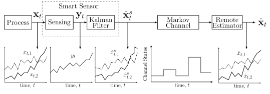
We consider a basic system setting wherein a smart sensor periodically samples, pre-estimates and sends its local estimation of a dynamic process to a remote estimator through a wireless link affected by random packet dropouts, as illustrated in Fig. 1.
II-A Process Model and Smart Sensor
The discrete-time linear time-invariant (LTI) model is given as (see e.g., [6, 21, 29])
| (1) | ||||
where is the process state vector, is the state transition matrix, is the measurement vector of the smart sensor attached to the process, is the measurement matrix, and are the process and measurement noise vectors, respectively. We assume and are independent and are identically distributed (i.i.d.) zero-mean Gaussian processes with corresponding covariance matrices and , respectively. In this work, we focus on the stability condition of the remote estimation of the process in the sense of average remote estimation mean-square error. Note that, if , then the covariance of is always bounded, and stability will trivially be satisfied. Thus, as commonly done in this context, in the sequel we focus on the more interesting case with indicating that the plant state grows up exponentially fast.
Note that in practice, feedback control of open-loop unstable LTI systems with Gaussian noise always requires sensors with unbounded measurement range, and adaptive zooming-in/zooming-out measurement range have been widely adopted [30]. Beyond the idealized situation of LTI systems, system models with exponentially growing modes are also obtained through linearization at unstable equilibria, see for example the Pendubot system in [27] and references therein.
Since the sensor’s measurements are noisy, a smart sensor is used to estimate the state of the process, . For that purpose a Kalman filter [21, 29] is used, which gives the minimum estimation MSE, based on the current and previous raw measurements:
| (2a) | ||||
| (2b) | ||||
| (2c) | ||||
| (2d) | ||||
| (2e) | ||||
where is the identity matrix, is the prior state estimate, is the posterior state estimate at time , is the Kalman gain. The matrices and represent the prior and posterior error covariance at the sensor at time , respectively. The first two equations above present the prediction steps while the last three equations correspond to the updating steps [31]. Note that is the output of the Kalman filter at time , i.e., the pre-filtered measurement of , with the estimation error covariance .
Assumption 1 ([6, 21, 22, 23, 24, 29]).
is observable and is controllable, i.e., the matrix concatenations and are of full rank.
Using Assumption 1, the local Kalman filter of system (1) is stable, i.e., the error covariance matrix converges to a finite matrix as the time index goes to infinity [31]. In the rest of the paper, we assume that the local Kalman filter operates in the steady state [6, 21, 22, 23, 24, 29], i.e., . Further, to simplify notation, the sensor’s estimation shall be denoted by .
II-B Wireless Channel
The main characteristic of the wireless fading channel is that the channel quality is a time-varying random process that changes over time in a correlated manner [7, 8, 9]. We consider a finite-state time-homogeneous Markov block-fading channel [7]. It is assumed that the channel power gain remains constant during the th time slot but may change slot by slot. We assume that the Markov channel has states, i.e,
The transition probability from state to state is time-homogeneous and given by
| (3) |
where . The matrix of channel state transition probability is given as
| (4) |
We assume that all the channel states are aperiodic and positive recurrent. Thus, the Markov chain induced by is ergodic [32].
We assume that the channel state information is available at both the sensor and the remote estimator, which can be achieved by standard channel estimation and feedback techniques, see e.g. [33] and the references therein. Let and denote the successful and failed packet detection of the remote estimator during time slot , respectively. The packet drop probability in channel state is
| (5) |
Note that the transmission is always perfect if , while no information-carrying packet is delivered to the remote estimator if . We define the packet drop probability matrix as
| (6) |
Example 1.
Suppose that the Markov channel has only two states, where the channel power gains, i.e., the effective signal-to-noise ratios (SNRs), are and . Assume the estimate-carrying packet has symbols and each symbol carries bits information. The minimum achievable packet drop rate is [34]
| (7) |
where ,
and is the SNR and is the Euler’s number. Taking , , and into (7), the packet drop probabilities are and .
In practice, the sensor can send a known sequence of symbols (called a pilot or channel training sequence) to the receiver, which can then estimate the channel power gain [35]. For the packet error probability at a certain channel condition, accurate value can be obtained by Monte Carlo simulation, i.e., sending a large sequence of packets to the receiver and calculate the ratio of failed packets.
II-C Remote Estimation and Stability Criteria
The smart sensor sends its local estimate to the remote estimator at every time slot. Each packet transmission has a unit delay that is equal to the sampling period of the system. For the considered fading model, packets may or may not arrive at the receiver due to the random packet dropouts. To account for packet transmission delays and the failures, the remote estimation of the current system states is based on the previously detected information packet. The optimal remote estimator in the sense of minimum mean-square error (MMSE) can be obtained as [6, 22]
| (8) |
Assuming a packet was successfully received at time , and the following transmission consecutively failed for times before the current time , i.e., , from (8), it can be obtained that , , and . Thus, (8) can be uniformly written as
| (9) |
where is the number of consecutive packet dropouts before time slot . In other words, can be treated as the age-of-information (AoI) of the remote estimator in time slot [36].
Then, the estimation error covariance is given as
| (10) | ||||
| (11) |
where (11) is obtained by substituting (9) and (1) into (10) and with:
| (12) |
Thus, the quality of the remote estimation error in time slot can be quantified via . We introduce the following function
| (13) |
From (11), we can write
| (14) |
Since is a countable stochastic process taking value from a countable infinity set
it will grow during periods of consecutive packet dropouts when . Since periods of consecutive packet dropouts have unbounded support, at best one can hope for some type of stochastic stability. In the present work, our focus is on the mean-square stability.
Definition 1 (Mean-Square Stability).
The remote estimation system is mean-square stable if and only if the average estimation MSE is bounded, where
| (15) |
and is the limit superior operator.
Note that establishing necessary and sufficient stability conditions is non-trivial as we consider correlated fading-channel model in the remote estimation system which induces a countable (and unbounded) Markov chain in the analysis. Some of the existing works adopt stochastic Lyapunov functions to elucidate such situations (see e.g., [15]). These however, merely lead to sufficient conditions.
III Main Results
In this section, we present and discuss the main results of the paper, which will be proved in Section V.
III-A The Necessary and Sufficient Stability Condition
Theorem 1.
Theorem 1 shows that the stability condition depends on the system matrix , the packet drop probability matrix and the matrix of the channel state transitions . It is important to note that the necessary and sufficient condition is determined by both the spectral radiuses of and the product of two matrices and . Since measures how fast the dynamic process varies, can be treated as an effective measurement of the Markov channel quality.
Remark 1.
In [15, Corollary 1], a sufficient condition in terms of exponential stability of a conventional-sensor-based remote estimation system over Markov channel is obtained as
| (17) |
where is the largest singular value of . Using Perron–Frobenius theorem [37], we have . In addition, due to the fact that the largest singular value is no smaller than the spectral radius, i.e., , it can be proved that the sufficient condition (17) is more restrictive than (16).
Corollary 1 (Special Case I).
Consider the same assumption and system model in Theorem 1. For the special case of i.i.d. packet dropout channel with packet dropout probability , the remote estimation system is mean-square stable if and only if the following condition holds:
| (18) |
Remark 2.
Corollary 2 (Special Case II).
Consider the same assumption and system model in Theorem 1. For the special case of Markovian packet dropout channel with packet dropout probability and and the channel state transition matrix
the remote estimation system is mean-square stable if and only if the following condition holds:
| (19) |
Remark 3.
For the Markovian on-off channel in Corollary 2, it is interesting to see that the stability condition only depends on one element of the -by- matrix , which is the state transition probability from the bad state to the bad state.
III-B Upper and Lower Bounds of the Estimation Error Function
A pair of asymptotic upper and lower bounds of the estimation error function are given below.
Proposition 1 (Asymptotic upper bound of the estimation-error function).
For any , there exists and such that
Proposition 2 (Asymptotic lower bound of the estimation-error function).
There exists a constant and such that .
Propositions 1 and 2 show that when a large number of consecutive packet dropouts occur, i.e., , the remote estimation error is upper and lower bounded by exponential functions in terms of .
Remark 4.
It can be observed that the estimation-error function grows as exponentially fast as .
IV Analysis of the Average Estimation MSE
In this section, we first investigate an estimation-cycle based performance analysis approach of the remote state estimation, and then develop new element-wise bounds of matrix powers. The results and technical lemmas obtained in this section will be used for the proofs of the main results of the paper.
As it is clear that Theorem 1 holds for the special cases with or , in the following we only focus on the cases with nor .
IV-A Stochastic Estimation-Cycle Based Analysis
Before analyzing the long-term average MSE of the remote estimation system and derive the stability condition, we need to introduce and analyze estimation cycle. To be specific, the th estimation cycle starts after the th successful transmission and ends at the th successful transmission as illustrated in Fig. 2. In other words, the estimation process is divided by the estimation cycles.
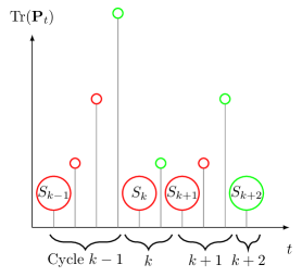
The channel state at the beginning of estimation cycle , i.e., a post-success channel state, is denoted by , where
| (21) |
is the set of post-success channel states and the cardinality of is . Without loss of generality, we assume that contains the first elements of . In other words, none of the last elements of can be a post-success channel state, while the others can.
Example 2.
Consider a two-state Markov channel with
and . It is clear that the channel states deterministically switches between the two states, and the transmission can be successful only in channel state 2. Thus, channel state 1 is the only post-success state, i.e., .
Then, we have the following property of .
Lemma 1.
is a time-homogeneous ergodic Markov chain with irreducible states of . The state transition matrix of is , which is the -by- matrix taken from the top-left corner of , where
| (22) |
and the last columns of are all zeros. The stationary distribution of is , which is the unique null-space vector of and , where .
Proof.
See Appendix A. ∎
Remark 5.
Our analysis investigates the sequence of successful reception instances. This has also been considered in [38], where the instances of successful reception are return times of a Markov chain. Different to [38], we focus on the channel states right after these instances, which form an ergodic Markov chain. Our approach will shed lights on the future work of the analysis of closed-loop control systems over Markov channels.
Let denote the sum number of transmissions in the th estimation cycle. The sum MSE in the th estimation cycle, say , is given as
| (23) |
From (15) it directly follows that the average estimation MSE can be rewritten as
| (24) |
Since is determined by , and the distribution of depends on and the distribution of is time-invariant, the unconditional distributions of and of are also time-invariant. We thus drop the time indexes of , and . Then, the time average of and can be translated to the following ensemble averages as
| (25) |
and
| (26) |
where is defined in Lemma 1 for and when .
From the definition of estimation cycle and the property of channel state transition, the conditional probability of the length of an estimation cycle is obtained as
| (27) |
If we now replace (27) into (25) and into (26), then after some algebraic manipulations, one can obtain:
| (28) | ||||
| (29) |
where
Taking (28) and (29) into (24), we have
| (30) |
Therefore, it turns out that the average estimation MSE depends on the estimation error function and the function , both of which involve matrix powers. In what follows, we will introduce and prove some technical lemmas about the element-wise upper and lower bounds of matrix powers, which are the key steps for analyzing the sufficient and necessary stability conditions of the remote estimation system.
IV-B Element-Wise Bounds of Matrix Powers
We give an element-wise upper bound of matrix powers as below.
Lemma 2 (Element-wise upper bound of matrix power).
Consider a -by- matrix with different eigenvalues , where , and define . Then, for any , there exist and such that
Proof.
See Appendix B. ∎
Definition 2 (Asymptotically and periodically lower bounded).
A function is asymptotically and periodically lower bounded by with a period if there exists such that
Thus, if is asymptotically and periodically lower bounded by with a period , then the sum of the function with a consecutive of samples is lower bounded by . When a direct lower bound of the function is intractable or very loose, we can resort to finding a periodical lower bound , which might introduce a tight lower bound of the average of per samples, i.e., . It is clear that the periodical lower bound is tighter if the period is smaller. In Lemma 3, we will show how to determine the period of a specific problem in details. Definition 2 will be used to capture the lower bound of the average sum MSE in (23) for analyzing the necessary stability condition.
Definition 3 (Asymptotically lower bounded).
A function is asymptotically lower bounded by if it is asymptotically and periodically lower bounded by with period .
Given the preceding definitions, we can obtain an element-wise lower bound of matrix powers as below.
Lemma 3 (Element-wise lower bound of matrix power).
(i) Consider a -by- matrix .
Then there exist and such that is asymptotically and periodically lower bounded by . The period is a positive integer no larger than the number of eigenvalues of with the same maximum magnitude.
(ii)
Consider a pair of -by- matrices and with the assumptions that is symmetric positive semidefinite and is controllable.
Then there exist and such that is asymptotically and periodically lower bounded by .
The period has the same property as in (i).
Proof.
See Appendix B. ∎
V Proof of the Main Results
V-A Proof of Proposition 1
V-B Proof of Proposition 2
V-C Proof of Theorem 1
Besides the upper and lower bounds of the estimation error function, to obtain the necessary and sufficient stability condition, we need some additional properties of and .
Lemma 4 (Property of matrix ).
Consider the stochastic matrix and the diagonal matrix defined in (4) and (6), respectively. Let and .
(i) If , there exists such that is asymptotically and periodically lower bounded by .
(ii) If , there exists , and such that is asymptotically and periodically lower bounded by .
(iii) .
Proof.
See Appendix C. ∎
Lemma 5 (Property of matrix ).
Proof.
See Appendix C. ∎
VI Numerical Results
In this section, we illustrate and compare the stability regions of the remote estimation system obtained using Theorem 1 of the current paper and based on Corollary 1 of our previous work [15]. We also present simulated results of the average estimation MSE in (24) based on the average of time steps.
We consider an example involving the Pendubot, a two-link planar robot [39]. A linearized continuous time model for balancing the Pendubot in the upright position can be found in [40]. With a sampling time of ms, we can then obtain the following discrete time model [27]:
| (36a) | |||
| (36b) | |||
| (36c) | |||
| (36d) | |||
Thus, and . Unless otherwise stated, we consider a two-state Markov channel model characterised by the transition matrix and conditional dropout probabilities , and .
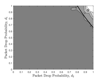
Fig. 3 shows the stability regions (in the dropout probability plane) for different and . In this figure, the solid and dashed line bounded regions are obtained from Theorem 1 and [15, Corollary 1], respectively. Specifically, we set in case (b), where and , and set and in cases (c) and (d), respectively. From cases (a)-(d), it is clear that our current necessary and sufficient stability region is much larger than the sufficient stability region established in [15]. Also, it can be observed that the necessary and sufficient stability region is convex in case (d) and is non-convex in cases (a)-(c). Note that the convexity of a stability region is important in practice. For example, if one has tested a set of communications parameter vectors that can stabilize the remote estimation system and the stability region is proved to be convex, any parameter vector that belong to the convex hull of the set can stabilize the system as well. Comparing (b) with (a), it is clear to see a smaller stability region as the system in (b) is more unstable than (a). Comparing (c) with (d), it is interesting to see that if the Markov channel has a longer memory, i.e., it has a higher chance to stay in a poor channel condition, then the remote estimation system has a smaller stability region.
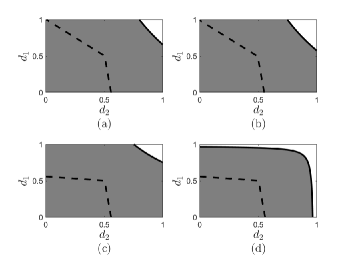
Fig. 4 shows the original unstable process of the system (36), and the remote estimation . We see that the estimator tracks the unstable process well, and the relative estimation error, i.e., decreases with time.
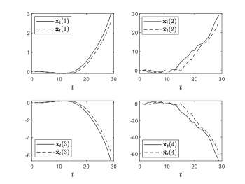
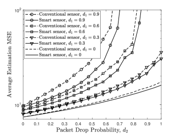
Fig. 5 shows the simulated average estimation MSEs of the smart-sensor-based and a conventional-sensor-based remote estimator [6] with different packet drop probabilities. Under the stability condition (illustrated as the gray area in Fig. 3(a)), we see that although the local estimator guarantees a better performance than the remote estimator, the performance gap is non-negligible only when the packet dropout probabilities are large at all channel states. It is interesting to note that the two cases actually have the same stability condition when packet dropout are i.i.d., see [6]. This motivates the hypothesis that the smart-sensor-based and the conventional-sensor-based remote estimation systems have the same stability condition under the Markov channel in terms of the LTI system transition matrix, the packet drop probabilities and the channel state transition matrix.
In Figs. 6 and 7, we give contour plots of the average estimation MSE in the smart-sensor-based and the conventional-sensor-based cases, respectively. It can be observed that the average estimation MSEs grow up dramatically outside the theoretical stability region (i.e., Fig. 3(a)) in both cases. This verifies the correctness of the stability condition and also implies that the stability condition of the two cases can be the same.

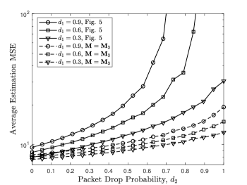
In Fig. 8, we consider a three-state Markov channel with the state transition matrix . Comparing with the two-state channel model considered in Fig. 5, a third channel state with a small packet drop rate is added. We see that the three-state channel case performs much better than the two-state channel one in terms of the average estimation MSE as the former channel is less error-prone.
VII Conclusions
In this paper, we have established the necessary and sufficient mean-square stability condition of a smart-sensor-based remote estimation system over a Markov fading channel, by developing the asymptotic theory of matrices which provides new (periodic) element-wise bounds of matrix powers. Our numerical results have verified the correctness of the stability condition and have shown that it is much more effective than existing sufficient conditions in the literature. It has been observed that the stability region in terms of the packet drop probabilities in different channel states can either be convex or non-convex depending on the transition probability matrix. Our simulation results have suggested that the stability conditions may coincide for schemes with a smart sensor and with a conventional sensor. This inspires our future work on analyzing the stability condition of the case without a smart sensor. Furthermore, the derived stability conditions can be used to design the optimal policy of transmission power control (e.g., via off-line design of ) as well as multi-sensor scheduling policies. In addition to stability, we will look into the performance of the smart sensor based remote estimation system and investigate the stationary distribution of estimation error covariances.
Furthermore, we will investigate the stability condition of the remote estimation system that adopts an aperiodic transmission policy. For example, an energy-constrained sensor normally uses an energy-saving protocol in practice that is to transmit only when the channel condition is good and/or the receiver has not received a packet for long time, i.e., with a large AoI state. We will extend the stochastic-estimation-cycle-based analytical approach to this case. Specifically, when analyzing the lengths of the stochastic estimation cycles, we will take into account how the transmission decisions depend on the current AoI state and the current channel conditions.
Appendix A: Proof of Lemma 1
The time homogeneousty of is clear due the time homogeneous Markov channel states. Let’s define the following sets , and denoting the channel states in which a packet transmission must succeed, can succeed or fail, and must fail, respectively. Since , the ‘can succeed’ state set . Due to the ergodicity of the Markov channel, it can be proved that given any current channel state, the hitting time of any state of is finite with a positive probability. Also, given a post-success state in , it is reachable from a state of in one step. Thus, given any state , the hitting time of any is finite with a positive probability. This completes the proof of the ergodicity of . Then, the stationary distribution is the solution of
| (37) |
where the state transition probability is . Let denote the hitting time from to , and and denotes the th row and th column of the matrix . We further have
| (38) | |||
| (39) |
which completes the proof of (22). From the definition of in (21), it is clear that the last columns of are all zeros, completing the proof of Lemma 1.
Appendix B: Proofs of Lemmas 2 and 3
VII-A Preliminaries
Assume a -by- matrix has different eigenvalues . Represent in its Jordan normal form of , where is a invertible matrix and
| (40) |
| (41) |
Let denote the size of Jordan block . Then, and can be represented as
| (42) | ||||
where and are -by matrices. Since is of full rank, and have full column rank of .
Then, we have
| (43) |
where
| (44) |
Note that has a full rank of for all if .
VII-B Proof of Lemma 2
The result follows upon noting that .
VII-C Proof of Lemma 3
Before proceeding to prove the element-wise lower bound of matrix powers, we need the following technical lemma.
Lemma 6.
Consider a -by- matrix with different eigenvalues , where , and a -by- symmetric and positive semidefinite matrix . If is controllable and for some , then .
Proof.
Assume that there exists such that . Then, we have
| (47) | ||||
| (48) | ||||
| (49) | ||||
| (50) |
where (48) is due to Sylvester’s rank inequality [41]. Thus, .
From the definitions of and , it is clear that
| (51) |
By multiplying on the both sides of (51), we have
| (52) |
Proof of Lemma 3(i).
If , is a full-rank square matrix and hence has a full row rank of . Since has a full column rank of , by using Sylvester’s rank inequality, we have
| (55) | ||||
Therefore, . From (45), we can find a pair of such that . Thus, without loss of generality, we assume that the dominant term of the polynomial is when , where and .
If and is the unique eigenvalue that has the maximum magnitude, it is clear that the dominant term of is . Thus, one can find such that is asymptotically lower bounded by .
If there are multiple eigenvalues having the same maximum magnitude, i.e., and , where , we consider the following two complementary cases:
Case 1): There exists such that and . In this case, the dominant term of is still . Thus, one can find such that is asymptotically lower bounded by .
Case 2): There exists a set with cardinality such that and . In this case, may not be asymptotically lower bounded by due to the multiple eigenvalues with identical magnitude but different phases.
In the following, we will show that is asymptotically and periodically bounded by . Let denote the index of the th eigenvalue in , where . Thus, , where . We have the following matrix
| (56) | ||||
where
| (57) |
and is a Vandermonde matrix, which is invertible due to the fact that for , see [42]. Let . Since is invertible, using the inequality of matrix-vector product [43, 44], we have
| (58) |
where is the minimum magnitude of the eigenvalues of . Since the largest magnitude of the elements of is no smaller than , we have
| (59) | ||||
and hence
| (60) | ||||
Therefore, is asymptotically and periodically lower bounded by with period , where is a positive constant. ∎
Proof of Lemma 3(ii).
From (45), if , it is easy to see that
| (61) |
where is a column vector determined by , and and is independent with . Thus, there exist such that ; otherwise, it violates Lemma 6. Then, by following the same steps of the proof of Lemma 3(i), we can prove that there exists such that is asymptotically and periodically lower bounded by . ∎
Appendix C: Proofs of Lemmas 4 and 5
VII-D Proof of Lemma 4
For part (i), since is an irreducible non-negative matrix and , the -by- matrix is also irreducible and non-negative, i.e., one can associate with the matrix a certain directed graph , which has exactly vertexes, and there is an edge from vertex to vertex precisely when , and is strongly connected. By using Lemma 3, there exists such that is asymptotically and periodically lower bounded by , where the period is no larger than the number of eigenvalues of with the same maximum magnitude. Then using the non-negative and irreducible property of , given , we can find such that is reachable from in steps, i.e., . Thus, if , we have
Since is asymptotically and periodically lower bounded by , is asymptotically and periodically lower bounded by . This completes the proof of part (i).
For part (ii), we construct a diagonal matrix , where if otherwise . Thus, is irreducible and non-negative. Since has all zero rows, the direct graph of , , can be generated by the strongly connected graph induced by and then remote the edges from vertexes . In other words, is part of . Then, it is easy to see that for any , we can find such that there exists a path from to in , otherwise, it violates the irreducible property of . Therefore, for any , there exist and such that . By using this property, part (ii) of Lemma 4 can be proved by following the similar steps of part (i).
For part (iii), since , and each element of is strictly less than , we have , . By using part (ii), i.e., there exist and such that is asymptotically and periodically lower bounded by , we have .
VII-E Proof of Lemma 5
For the case that , since and is a stochastic matrix, there exists such that . Using Lemma 4(i), for any , is asymptotic and periodically lower bounded by . Thus, there exists such that
For the case that , given any , we can find such that . Using Lemma 4(ii), there exists such that is asymptotic and periodically lower bounded by . Thus, there exists , and such that, also in this case, .
Appendix D: Proof of Theorem 1
Using the property that is a monotonically increasing function [22], from (23), we have
| (62) |
Then, we consider two scenarios: (i) all channel states are post-success states, i.e., and ; and (ii) some channel states are not post-success states, i.e., and .
(i) . Using Proposition 1, Lemma 2 and the inequality (62), for any , we can find such that in (29) is upper bounded as
| (63) |
where , and is a constant. Thus, is bounded if . By using Proposition 2 and Lemma 5 and after some algebraic manipulations, there exists such that in (29)
| (64) |
where , and is a constant. Thus, if is bounded. Therefore, is bounded if and only if . Similarly, since given in Lemma 4(iii), it can be proved that is always bounded.
Therefore, is bounded if and only if holds. This completes the proof of Theorem 1 in scenario (i).
(ii) . It is clear that the upper bound in scenario (ii) is the same as in (63). Different from scenario (i), the lower bound cannot be obtained as in (64) directly since making the lower bound useless in scenario (ii).
Taking Proposition 2 and (62) into (29), there exists such that
| (65) | ||||
where is a constant. Due to the ergodicity of the Markov channel, for any non-post-success state in , there exists a post-success state in such that can transit to after a finite number of failure transmissions, where . In other words, for any , there exists such that the th column of the matrix
is not of all zeros and has a positive entry of . Then, we have
| (66) | ||||
Applying (66) into (65) for times, it can be obtained as
| (67) | ||||
Letting
and following the same steps in scenario (i), the proof of Theorem 1 in scenario (ii) is completed.
References
- [1] I. Akyildiz, W. Su, Y. Sankarasubramaniam, and E. Cayirci, “Wireless sensor networks: a survey,” Computer Networks, vol. 38, no. 4, pp. 393–422, 2002.
- [2] F. Alam, R. Mehmood, I. Katib, N. N. Albogami, and A. Albeshri, “Data fusion and IoT for smart ubiquitous environments: A survey,” IEEE Access, vol. 5, pp. 9533–9554, 2017.
- [3] J. Lee, B. Bagheri, and H.-A. Kao, “A cyber-physical systems architecture for industry 4.0-based manufacturing systems,” Manufacturing Letters, vol. 3, pp. 18 – 23, 2015.
- [4] K. Antonakoglou, X. Xu, E. Steinbach, T. Mahmoodi, and M. Dohler, “Toward haptic communications over the 5G tactile Internet,” IEEE Commun. Surveys Tuts., vol. 20, no. 4, pp. 3034–3059, 2018.
- [5] T. N. Theis and H.-S. P. Wong, “The end of Moore’s law: A new beginning for information technology,” Computing in Science & Engineering, vol. 19, no. 2, p. 41, 2017.
- [6] L. Schenato, “Optimal estimation in networked control systems subject to random delay and packet drop,” IEEE Trans. Autom. Control, vol. 53, no. 5, pp. 1311–1317, Jun. 2008.
- [7] P. Sadeghi, R. A. Kennedy, P. B. Rapajic, and R. Shams, “Finite-state Markov modeling of fading channels - a survey of principles and applications,” IEEE Signal Process. Mag., vol. 25, no. 5, pp. 57–80, Sep. 2008.
- [8] Q. Zhang and S. A. Kassam, “Finite-state Markov model for Rayleigh fading channels,” IEEE Trans. Commun., vol. 47, no. 11, pp. 1688–1692, 1999.
- [9] C. C. Tan and N. C. Beaulieu, “On first-order Markov modeling for the Rayleigh fading channel,” IEEE Trans. Commun., vol. 48, no. 12, pp. 2032–2040, 2000.
- [10] B. Sinopoli, L. Schenato, M. Franceschetti, K. Poolla, M. I. Jordan, and S. S. Sastry, “Kalman filtering with intermittent observations,” IEEE Trans. Autom. Control, vol. 49, no. 9, pp. 1453–1464, Sep. 2004.
- [11] L. Xie and L. Xie, “Stability of a random Riccati equation with Markovian binary switching,” IEEE Trans. Autom. Control, vol. 53, no. 7, pp. 1759–1764, Aug 2008.
- [12] M. Huang and S. Dey, “Stability of Kalman filtering with Markovian packet losses,” Automatica, vol. 43, no. 4, pp. 598 – 607, 2007.
- [13] N. Xiao, L. Xie, and M. Fu, “Kalman filtering over unreliable communication networks with bounded Markovian packet dropouts,” International Journal of Robust and Nonlinear Control, vol. 19, no. 16, pp. 1770–1786, 11 2009.
- [14] K. You, M. Fu, and L. Xie, “Mean square stability for Kalman filtering with Markovian packet losses,” Automatica, vol. 47, no. 12, pp. 2647–2657, Dec 2011.
- [15] D. E. Quevedo, A. Ahlen, and K. H. Johansson, “State estimation over sensor networks with correlated wireless fading channels,” IEEE Trans. Autom. Control, vol. 58, no. 3, pp. 581–593, Mar. 2013.
- [16] J. Chakravorty and A. Mahajan, “Remote estimation over a packet-drop channel with markovian state,” IEEE Transactions on Automatic Control, vol. 65, no. 5, pp. 2016–2031, 2019.
- [17] Y. Z. Lun, C. Rinaldi, A. Alrish, A. D’Innocenzo, and F. Santucci, “On the impact of accurate radio link modeling on the performance of wirelesshart control networks,” in IEEE INFOCOM 2020-IEEE Conference on Computer Communications. IEEE, 2020, pp. 2430–2439.
- [18] K. Huang, W. Liu, Y. Li, B. Vucetic, and A. Savkin, “Optimal downlink-uplink scheduling of wireless networked control for Industrial IoT,” IEEE Internet Things J., vol. 7, no. 3, pp. 1756–1772, Mar. 2020.
- [19] B. Hu, Y. Wang, P. V. Orlik, T. Koike-Akino, and J. Guo, “Co-design of safe and efficient networked control systems in factory automation with state-dependent wireless fading channels,” Automatica, vol. 105, pp. 334–346, 2019.
- [20] P. Minero, L. Coviello, and M. Franceschetti, “Stabilization over markov feedback channels: the general case,” IEEE Trans. Autom. Control, vol. 58, no. 2, pp. 349–362, 2012.
- [21] L. Shi and L. Xie, “Optimal sensor power scheduling for state estimation of Gauss-Markov systems over a packet-dropping network,” IEEE Trans. Signal Process., vol. 60, no. 5, pp. 2701–2705, May 2012.
- [22] L. Shi and H. Zhang, “Scheduling two Gauss-Markov systems: An optimal solution for remote state estimation under bandwidth constraint,” IEEE Trans. Signal Process., vol. 60, no. 4, pp. 2038–2042, Apr. 2012.
- [23] S. Wu, X. Ren, S. Dey, and L. Shi, “Optimal scheduling of multiple sensors over shared channels with packet transmission constraint,” Automatica, vol. 96, pp. 22–31, 2018.
- [24] A. S. Leong, S. Dey, and D. E. Quevedo, “Sensor scheduling in variance based event triggered estimation with packet drops,” IEEE Trans. Autom. Control, vol. 62, no. 4, pp. 1880–1895, Apr. 2017.
- [25] Y. Li, L. Shi, P. Cheng, J. Chen, and D. E. Quevedo, “Jamming attacks on remote state estimation in cyber-physical systems: A game-theoretic approach,” IEEE Trans. Autom. Control, vol. 60, no. 10, pp. 2831–2836, 2015.
- [26] K. Ding, Y. Li, D. E. Quevedo, S. Dey, and L. Shi, “A multi-channel transmission schedule for remote state estimation under DoS attacks,” Automatica, vol. 78, pp. 194 – 201, 2017.
- [27] A. S. Leong, D. E. Quevedo, D. Dolz, and S. Dey, “Transmission scheduling for remote state estimation over packet dropping links in the presence of an eavesdropper,” IEEE Transactions on Automatic Control, vol. 64, no. 9, pp. 3732–3739, 2019.
- [28] K. Huang, W. Liu, Y. Li, and B. Vucetic, “To retransmit or not: Real-time remote estimation in wireless networked control,” in Proc. IEEE ICC, May 2019, pp. 1–7.
- [29] C. Yang, J. Wu, W. Zhang, and L. Shi, “Schedule communication for decentralized state estimation,” IEEE Trans. Signal Process., vol. 61, no. 10, pp. 2525–2535, May 2013.
- [30] G. N. Nair, F. Fagnani, S. Zampieri, and R. J. Evans, “Feedback control under data rate constraints: An overview,” Proc. IEEE, vol. 95, no. 1, pp. 108–137, Jan. 2007.
- [31] P. S. Maybeck, Stochastic Models, Estimation, and Control. Academic press, 1982, vol. 3.
- [32] R. Durrett, Probability: Theory and Examples. Cambridge university press, 2019, vol. 49.
- [33] S. Coleri, M. Ergen, A. Puri, and A. Bahai, “Channel estimation techniques based on pilot arrangement in OFDM systems,” IEEE Trans. Broadcast., vol. 48, no. 3, pp. 223–229, 2002.
- [34] Y. Polyanskiy, H. V. Poor, and S. Verdu, “Channel coding rate in the finite blocklength regime,” IEEE Trans. Inf. Theory, vol. 56, no. 5, pp. 2307–2359, May 2010.
- [35] D. Tse and P. Viswanath, Fundamentals of wireless communication. Cambridge university press, 2005.
- [36] S. Kaul, R. Yates, and M. Gruteser, “Real-time status: How often should one update?” in Proc. IEEE INFOCOM, Mar. 2012, pp. 2731–2735.
- [37] H. Minc, Nonnegative Matrices. Wiley, 1988.
- [38] D. E. Quevedo, W.-J. Ma, and V. Gupta, “Anytime control using input sequences with Markovian processor availability,” IEEE Trans. Autom. Control, vol. 60, no. 2, pp. 515–521, Feb. 2015.
- [39] M. W. Spong and D. J. Block, “The pendubot: a mechatronic system for control research and education,” in Proc. IEEE CDC, 1995, pp. 555–556 vol.1.
- [40] D. J. Block and M. W. Spong, “Mechanical design and control of the pendubot,” SAE trans., pp. 36–43, 1995.
- [41] G. Strang, Introduction to Linear Algebra. Wellesley-Cambridge Press Wellesley, MA, 1993, vol. 3.
- [42] H. Roger and R. J. Charles, Topics in Matrix Analysis. Cambridge University Press, 1994.
- [43] J. F. Grcar, “A matrix lower bound,” Linear Algebra and its Applications, vol. 433, no. 1, pp. 203–220, 2010.
- [44] J. Von Neumann and H. H. Goldstine, “Numerical inverting of matrices of high order,” Bulletin of the American Mathematical Society, vol. 53, no. 11, pp. 1021–1099, 1947.
![[Uncaptioned image]](https://cdn.awesomepapers.org/papers/ec08a7e1-887d-4c46-b126-46aaa0bbe8f1/Wanchun.jpg) |
Wanchun Liu (M’18) received the B.S. and M.S.E. degrees in electronics and information engineering from Beihang University, Beijing, China, and Ph.D. from The Australian National University, Canberra, Australia. She is currently a Postdoctoral Research Associate at the University of Sydney. Her research interest lies in ultra-reliable low-latency communications and wireless networked control systems for industrial Internet of Things (IIoT). She was a recipient of the Chinese Government Award for Outstanding Students Abroad 2017. She is a co-chair of the Australian Communication Theory Workshop since 2020. |
![[Uncaptioned image]](https://cdn.awesomepapers.org/papers/ec08a7e1-887d-4c46-b126-46aaa0bbe8f1/Daniel.jpg) |
Daniel E. Quevedo (S’97–M’05–SM’14–F’21) received Ingeniero Civil Electrónico and M.Sc. degrees from Universidad Técnica Federico Santa María, Valparaíso, Chile, in 2000, and in 2005 the Ph.D. degree from the University of Newcastle, Australia. He is Professor of Cyberphysical Systems at the School of Electrical Engineering and Robotics, Queensland University of Technology (QUT), in Australia. Before joining QUT, he established and led the Chair in Automatic Control at Paderborn University, Germany. In 2003 he received the IEEE Conference on Decision and Control Best Student Paper Award and was also a finalist in 2002. He is co-recipient of the 2018 IEEE Transactions on Automatic Control George S. Axelby Outstanding Paper Award. Prof. Quevedo currently serves as Associate Editor for IEEE Control Systems and in the Editorial Board of the International Journal of Robust and Nonlinear Control. From 2015–2018 he was Chair of the IEEE Control Systems Society Technical Committee on Networks & Communication Systems. His research interests are in networked control systems, control of power converters and cyberphysical systems security. |
![[Uncaptioned image]](https://cdn.awesomepapers.org/papers/ec08a7e1-887d-4c46-b126-46aaa0bbe8f1/Yonghui.jpg) |
Yonghui Li (M’04-SM’09-F’19) received his PhD degree in November 2002 from Beijing University of Aeronautics and Astronautics. From 1999 – 2003, he was affiliated with Linkair Communication Inc, where he held a position of project manager with responsibility for the design of physical layer solutions for the LAS-CDMA system. Since 2003, he has been with the Centre of Excellence in Telecommunications, the University of Sydney, Australia. He is now a Professor in School of Electrical and Information Engineering, University of Sydney. He is the recipient of the Australian Queen Elizabeth II Fellowship in 2008 and the Australian Future Fellowship in 2012. His current research interests are in the area of wireless communications, with a particular focus on MIMO, millimeter wave communications, machine to machine communications, coding techniques and cooperative communications. He holds a number of patents granted and pending in these fields. He is now an editor for IEEE transactions on communications and IEEE transactions on vehicular technology. He also served as a guest editor for several special issues of IEEE journals, such as IEEE JSAC special issue on Millimeter Wave Communications. He received the best paper awards from IEEE International Conference on Communications (ICC) 2014, IEEE PIMRC 2017 and IEEE Wireless Days Conferences (WD) 2014. |
![[Uncaptioned image]](https://cdn.awesomepapers.org/papers/ec08a7e1-887d-4c46-b126-46aaa0bbe8f1/Kalle.jpg) |
Karl Henrik Johansson (SM’08-F’13) is Professor at the School of Electrical Engineering and Computer Science, KTH Royal Institute of Technology, Sweden. He received MSc and PhD degrees from Lund University. He has held visiting positions at UC Berkeley, Caltech, NTU, HKUST Institute of Advanced Studies, and NTNU. His research interests are in networked control systems, cyber-physical systems, and applications in transportation, energy, and automation. He is a member of the Swedish Research Council’s Scientific Council for Natural Sciences and Engineering Sciences. He has served on the IEEE Control Systems Society Board of Governors, the IFAC Executive Board, and is currently Vice-President of the European Control Association Council. He has received several best paper awards and other distinctions from IEEE, IFAC, and ACM. He has been awarded Distinguished Professor with the Swedish Research Council and Wallenberg Scholar with the Knut and Alice Wallenberg Foundation. He has received the Future Research Leader Award from the Swedish Foundation for Strategic Research and the triennial Young Author Prize from IFAC. He is Fellow of the IEEE and the Royal Swedish Academy of Engineering Sciences, and he is IEEE Control Systems Society Distinguished Lecturer. |
![[Uncaptioned image]](https://cdn.awesomepapers.org/papers/ec08a7e1-887d-4c46-b126-46aaa0bbe8f1/Branka.jpg) |
Branka Vucetic (F’03) received the BSEE, MSEE and PhD degrees in 1972, 1978 and 1982, respectively, in Electrical Engineering, from The University of Belgrade, Belgrade. She is an ARC Laureate Fellow and Director of the Centre of Excellence for IoT and Telecommunications at the University of Sydney. Her current work is in the areas of wireless networks and Internet of Things. In the area of wireless networks, she explores ultra-reliable, low-latency techniques and transmission in millimetre wave frequency bands. In the area of the Internet of things, Vucetic works on providing wireless connectivity for mission critical applications. Branka Vucetic is a Fellow of IEEE, the Australian Academy of Science and the Australian Academy of Technological Sciences and Engineering. |