5cm \cftsetrmarg6cm \settocbibnameReferences
Representing and Learning
Functions Invariant Under Crystallographic Groups
Abstract
Crystallographic groups describe the symmetries of crystals and other repetitive structures encountered in nature and the sciences. These groups include the wallpaper and space groups. We derive linear and nonlinear representations of functions that are (1) smooth and (2) invariant under such a group. The linear representation generalizes the Fourier basis to crystallographically invariant basis functions. We show that such a basis exists for each crystallographic group, that it is orthonormal in the relevant space, and recover the standard Fourier basis as a special case for pure shift groups. The nonlinear representation embeds the orbit space of the group into a finite-dimensional Euclidean space. We show that such an embedding exists for every crystallographic group, and that it factors functions through a generalization of a manifold called an orbifold. We describe algorithms that, given a standardized description of the group, compute the Fourier basis and an embedding map. As examples, we construct crystallographically invariant neural networks, kernel machines, and Gaussian processes.
1 Introduction
Among the many forms of symmetry observed in nature, those that arise from repetitive spatial patterns are particularly important. These are described by sets of transformations of Euclidean space called crystallographic groups [65, 62]. For example, consider a problem in materials science, where atoms are arranged in a crystal lattice. The symmetries of the lattice are then characterized by a crystallographic group . Symmetry means that, if we apply one of the transformations in to move the lattice—say to rotate or shift it—the transformed lattice is indistinguishable from the untransformed one. In such a lattice, the Coulomb potential acting on any single electron due to a collection of fixed nuclei does not change under any of the transformations in [12, 42, 36]. If we think of the potential field as a function on , this is an example of a -invariant function, i.e., a function whose values do not change if its arguments are transformed by elements of the group. When solving the resulting Schrödinger equation for single particle states, members of the group commute with the Hamiltonian, and quantum observables are again -invariant [12, 37, 36, 57, 42, 26]. A different example are ornamental tilings on the walls of the Alhambra, which, when regarded as functions on , are invariant under two-dimensional crystallographic groups [58]. The purpose of this work is to construct smooth invariant functions for any given crystallographic group in any dimension.
For finite groups, invariant functions can be constructed easily by summing over all group elements; for compact infinite groups, the sum can be replaced by an integral. This and related ideas have received considerable attention in machine learning [e.g., 38, 21, 14]. Such summations are not possible for crystallographic groups, which are neither finite nor compact, but their specific algebraic and geometric properties allow us to approach the problem in a different manner. We postpone a detailed literature review to Section 10, and use the remainder of this section to give a non-technical sketch of our results.
1.1. A non-technical overview
This section sketches our results in a purely heuristic way; proper
definitions follow in Section 2.
Crystallographic symmetry.
Crystallographic groups are groups that tile a Euclidean space with a convex shape.
Suppose we place a convex polytope in the space , say a square or a rectangle in the plane.
Now make a copy of , and use a transformation to
move this copy to another location.
We require that is an isometry, which means it may shift, rotate or flip , but does not
change its shape or size.
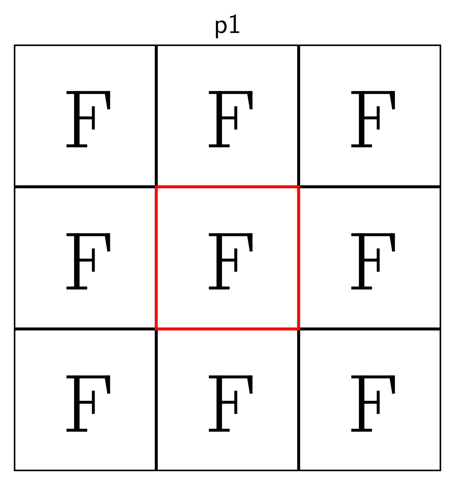
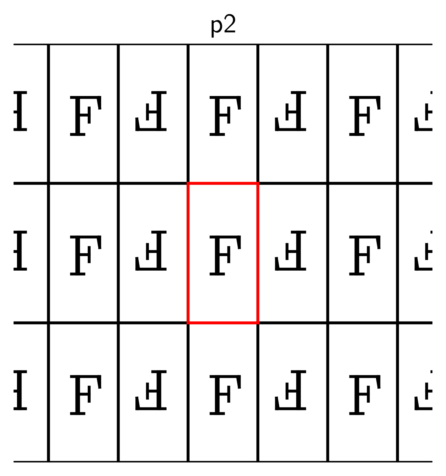
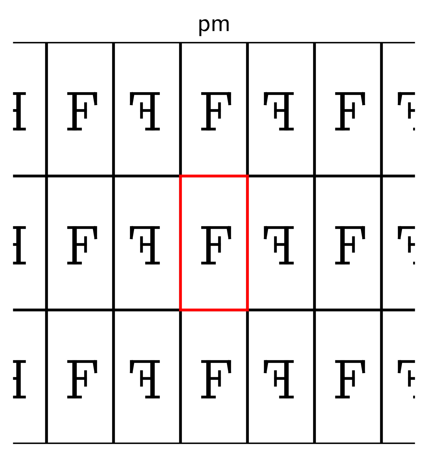
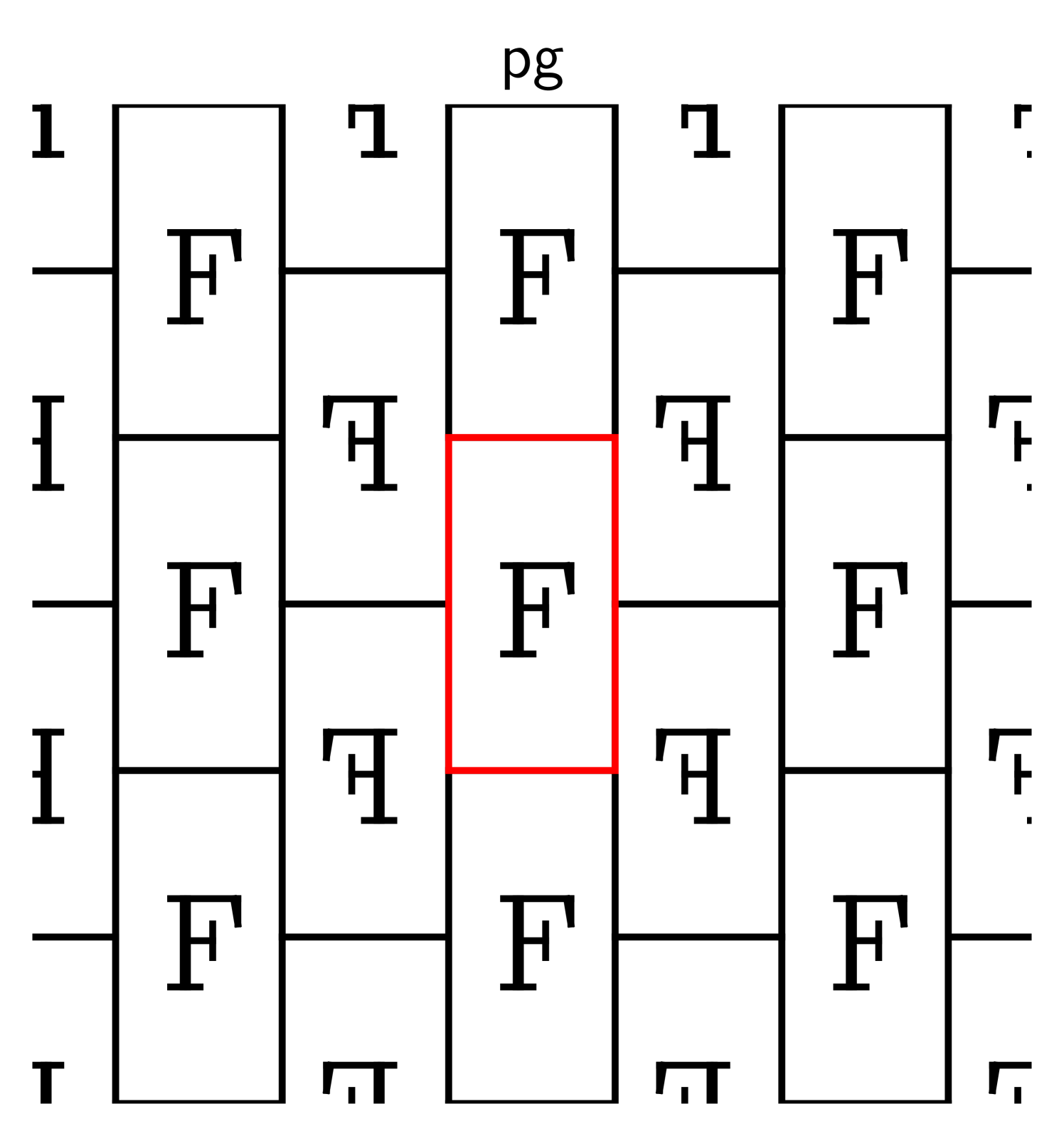
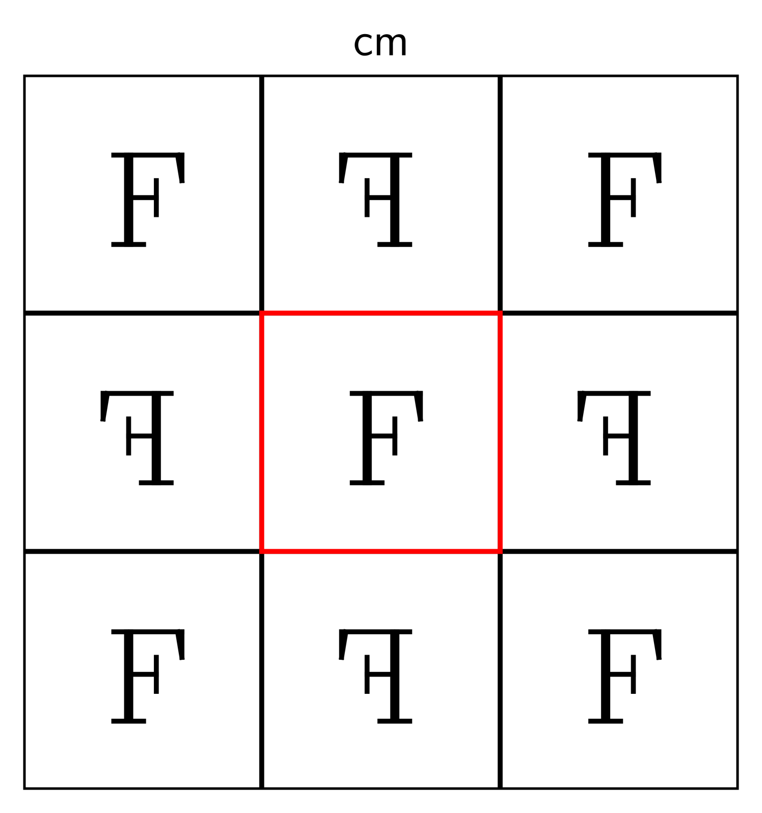
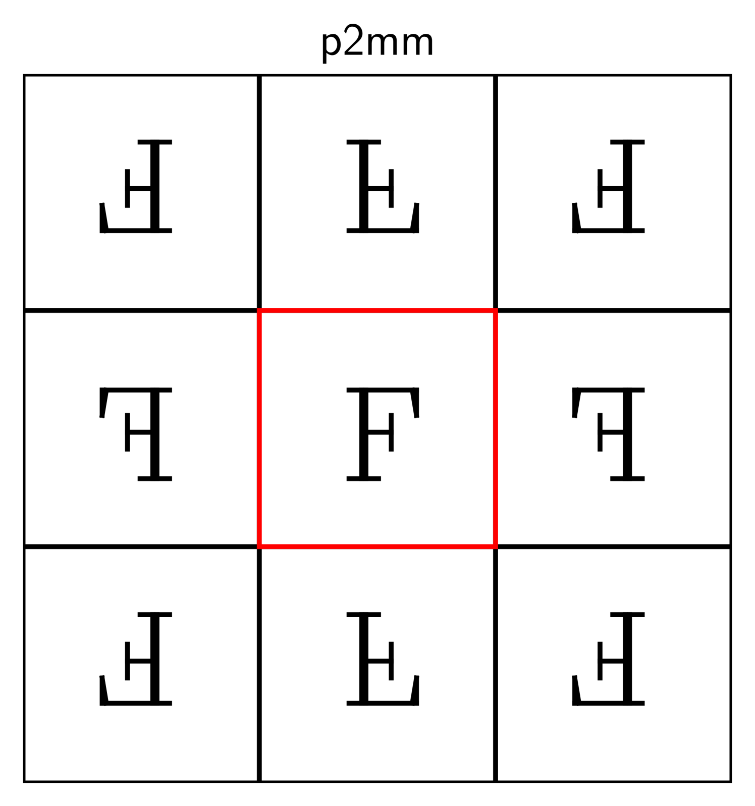
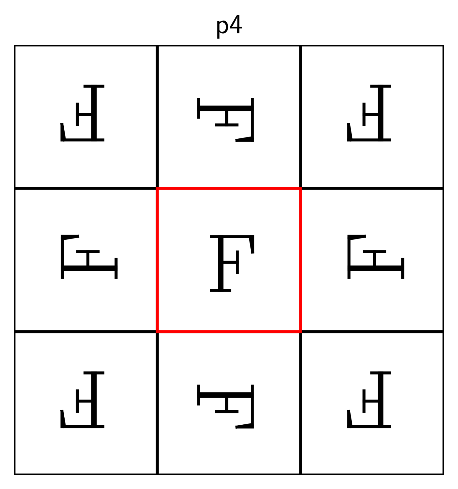
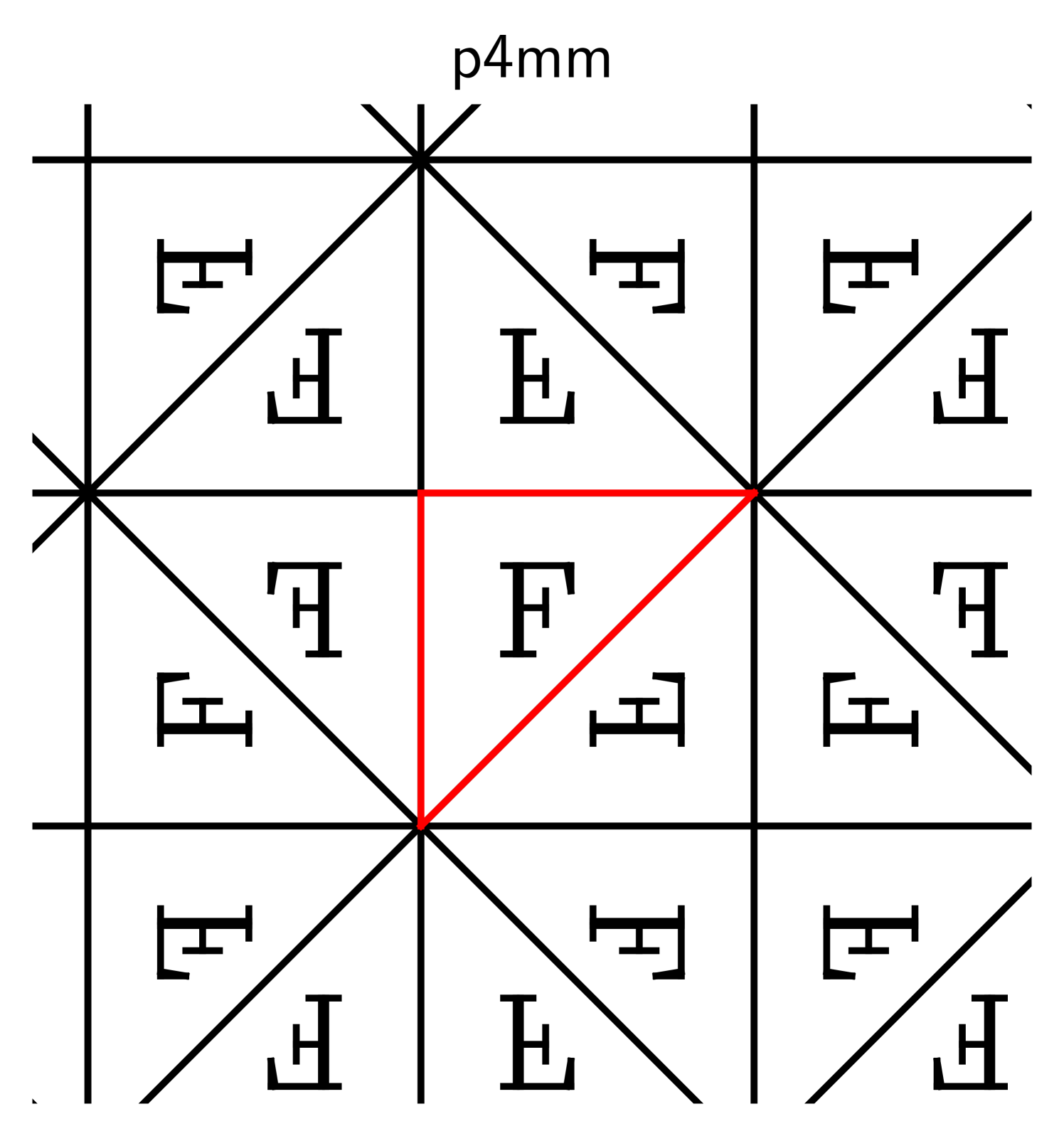
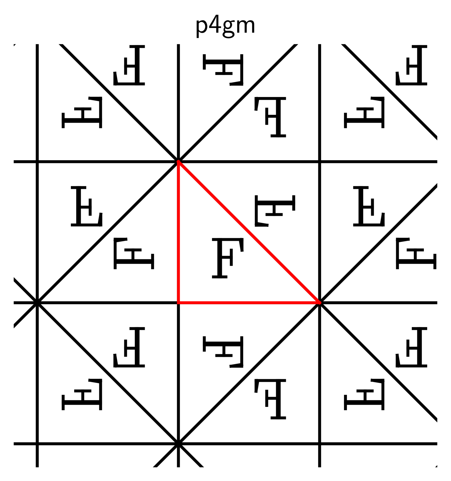
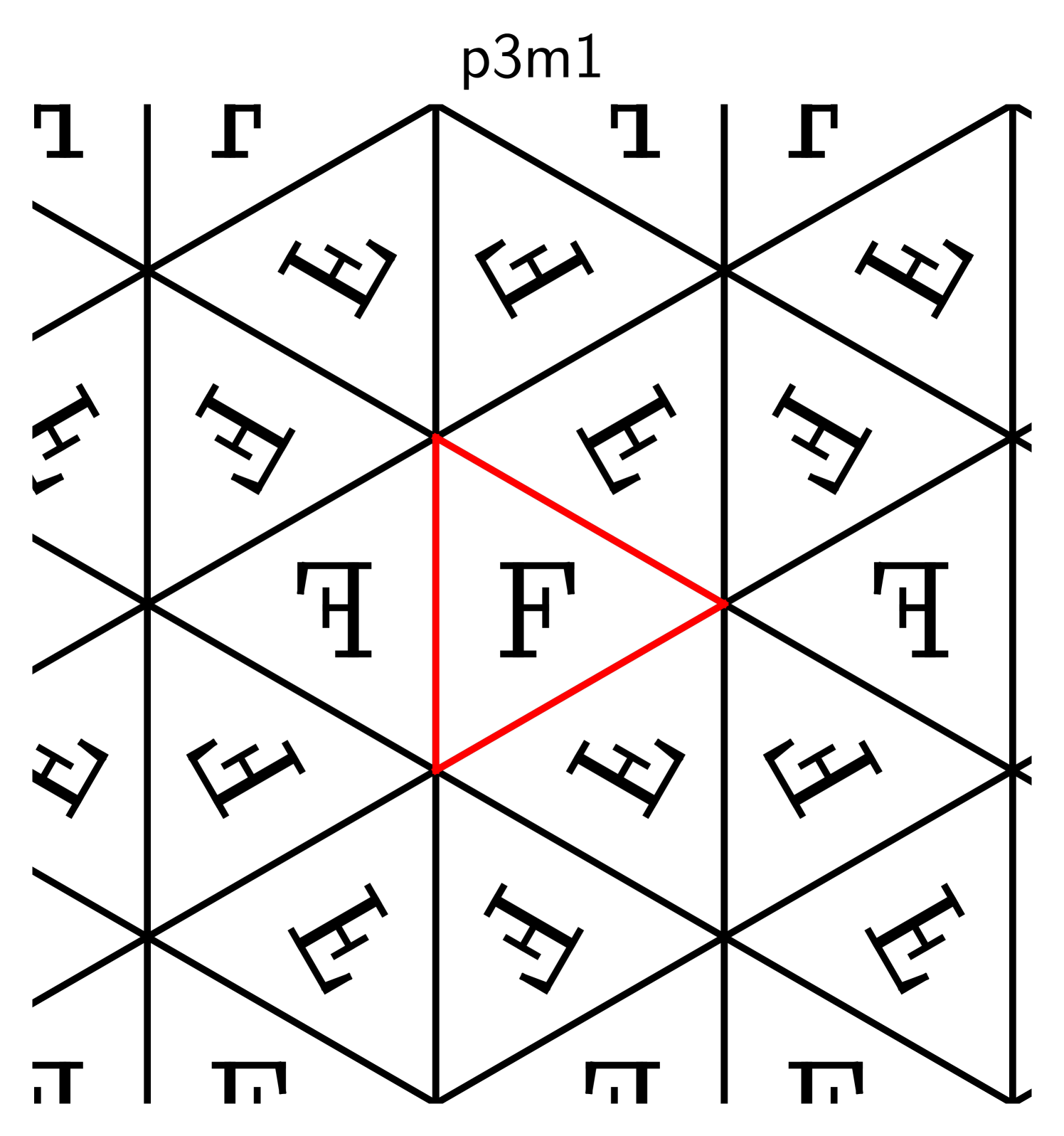
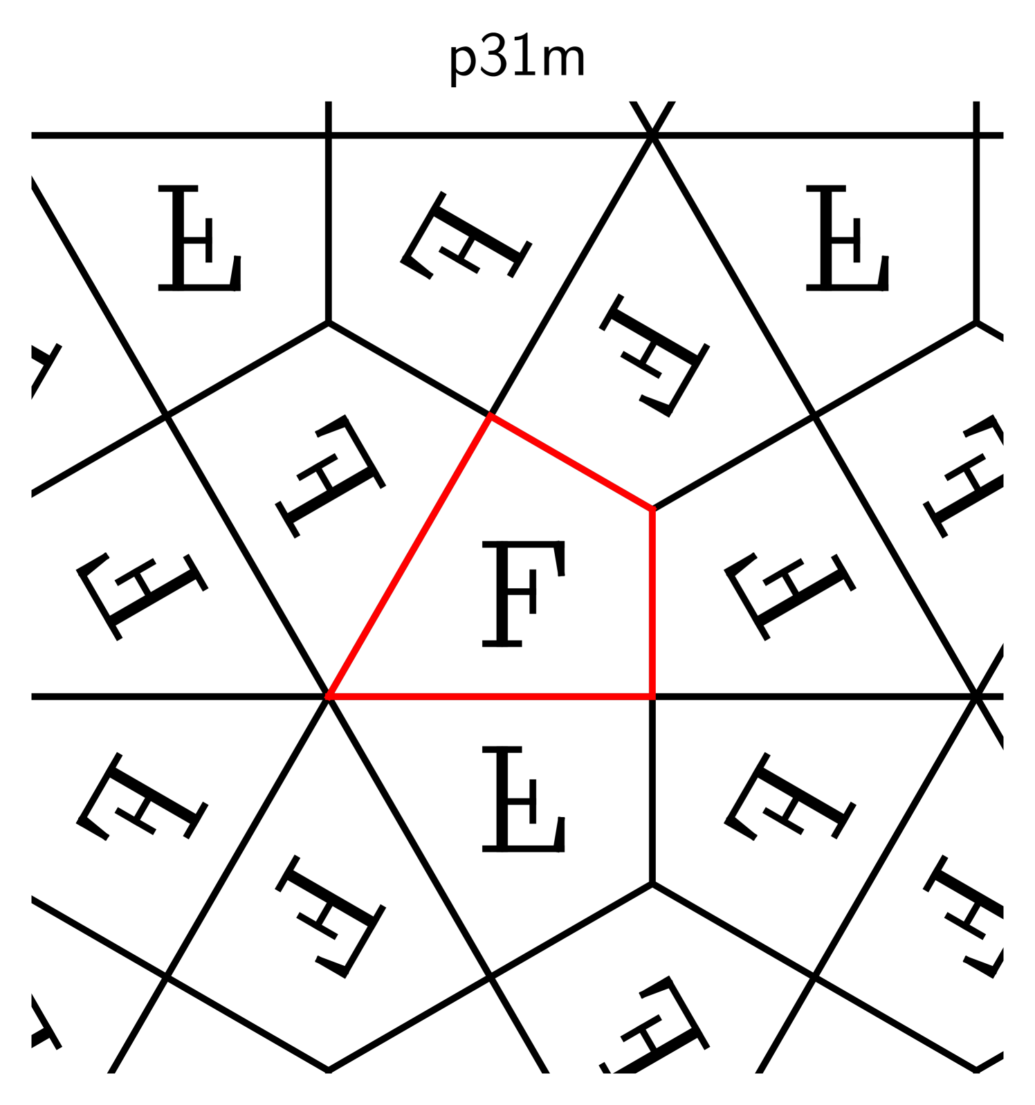
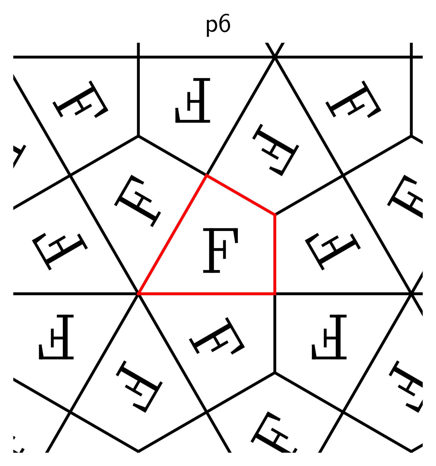
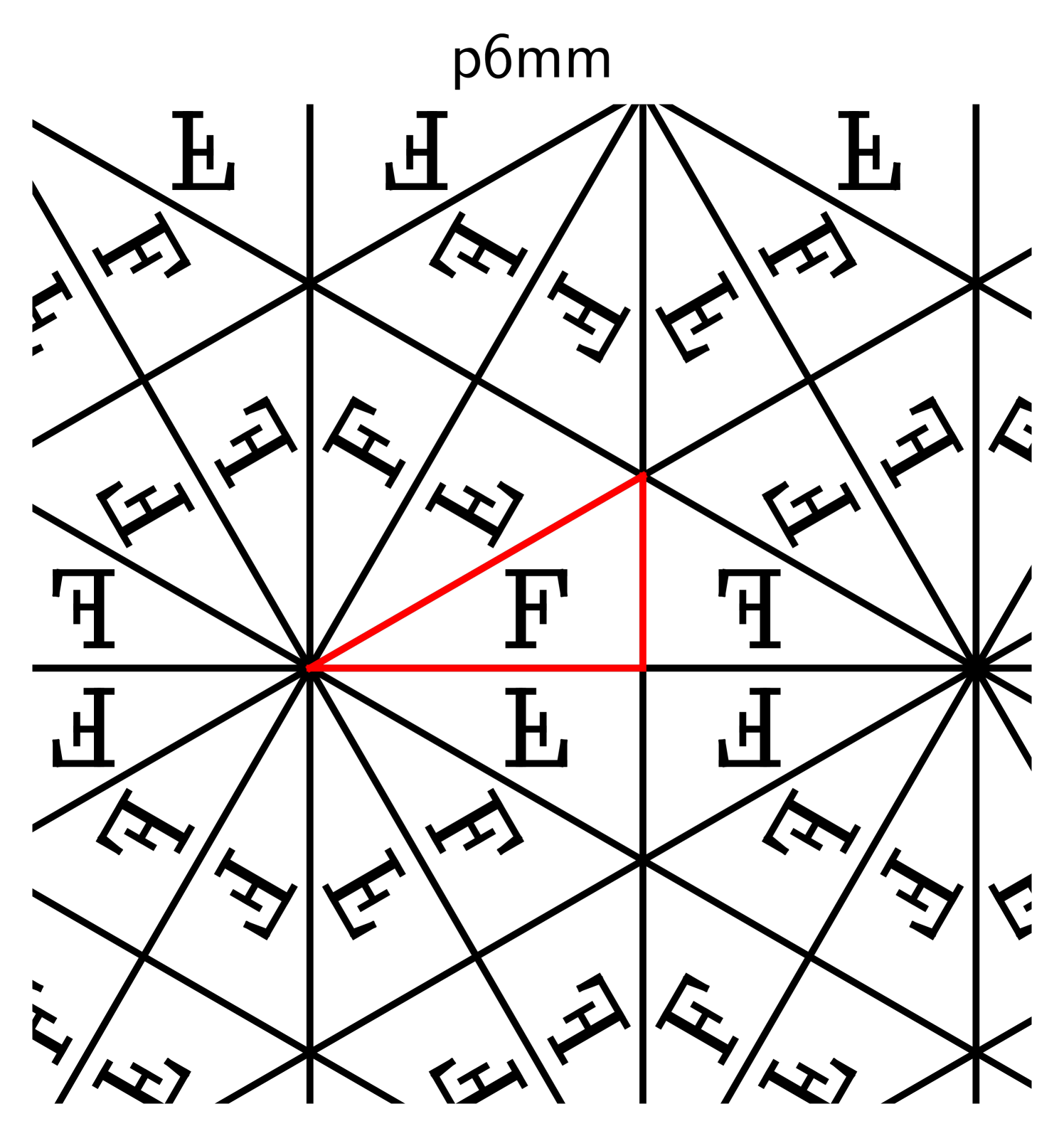
Here are some examples, where the original shape is marked in red:
The descriptors p1, p2, and p2mm follow the naming standard for groups
developed by crystallographers [31], and the symbol “F” is inscribed
to clarify which transformations are used.
The transformations in these examples are horizontal and vertical shifts (in p1), rotations around the
corners of the rectangle in (p2), and reflections about its edges (p2mm).
Suppose we repeat one of these processes indefinitely so that the copies of cover the entire plane
and overlap only on their boundaries. That requires a countably infinite number of
transformations, one per copy. Collect these into a set .
If this set forms a group, this group is called crystallographic.
Such groups describe all possible symmetries of crystals, and have been thoroughly studied in
crystallography. For each dimension , there is—up to a natural notion of isomorphy that we explain in Section 2—only
a finite number of crystallographic groups: Two on , 17 on ,
230 on , and so forth.
Those on are also known as wallpaper groups, and those on as space groups.
The objects of interest.
A function is invariant under if it satisfies
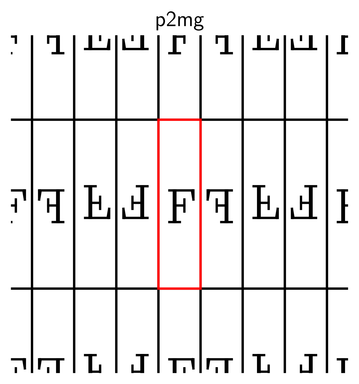
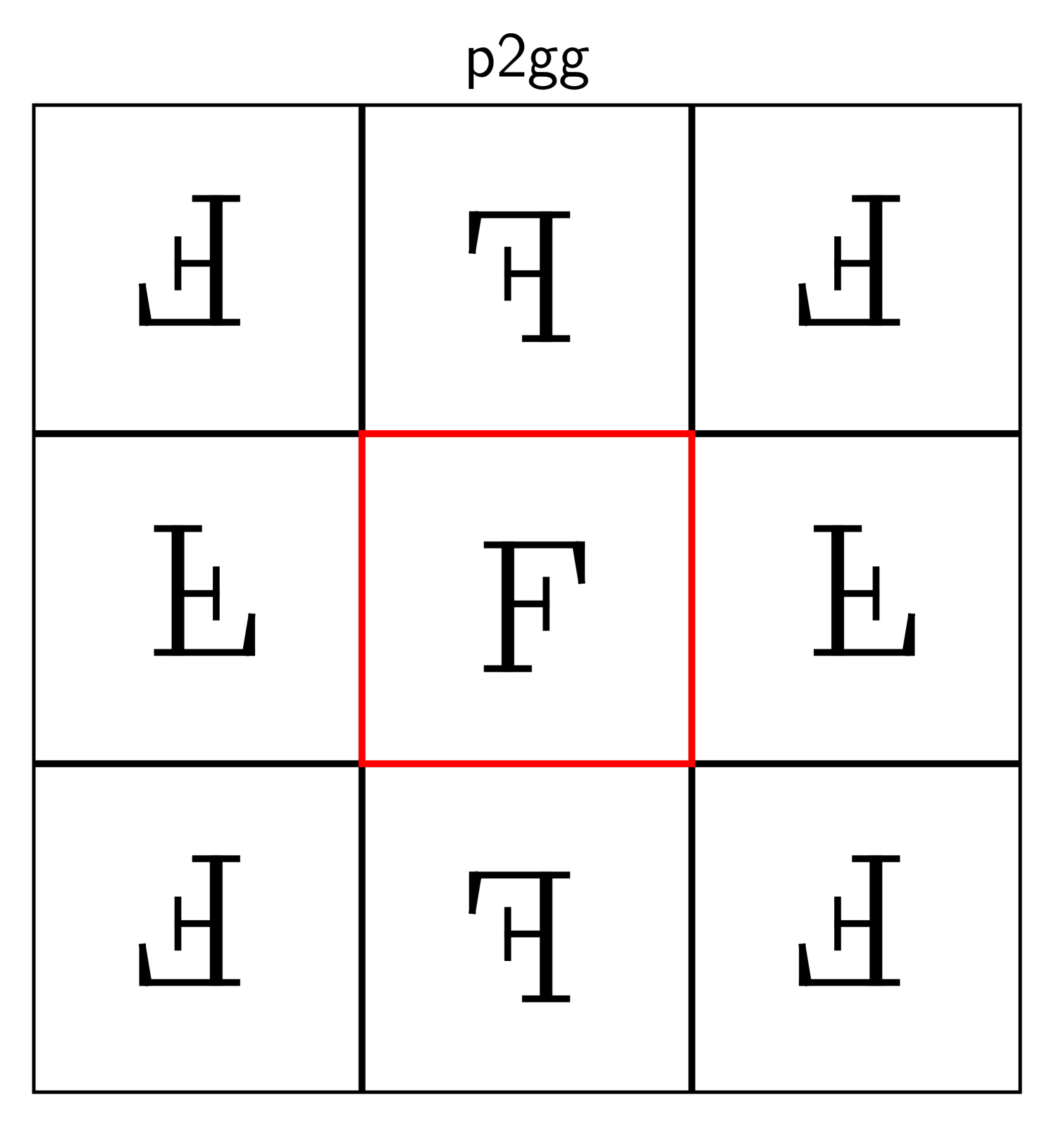
A simple way to construct such a function is to start with a tiling as above, define a function on , and then replicate it on every copy of . Here are two examples on , corresponding to (ii) and (iii) above, and an example on :
However, as the examples illustrate, functions obtained this way are typically not continuous. Our goal is to construct smooth invariant functions, such as these:
We identify two representations of such functions, one linear and one nonlinear.
Working with either representation algorithmically requires a data structure representing the invariance
constraint. We construct such a structure, which we call an orbit graph,
in Section 4. This graph is constructed from a description of the group
(which can be encoded as a finite set of matrices) and of (a finite set of vectors).
Linear representations: Invariant Fourier transforms.
We are primarily interested in two and three dimensions, but a one-dimensional example
is a good place to start: In one dimension, a convex polytope is always an interval, say . If we choose
as the group of all shifts of integer length, it tiles the line with .
In this case, an invariant function is simply a periodic function with period . Smooth periodic
functions can be represented as a Fourier series,
for sequences of scalar coefficients and . Note each sine and cosine on the right is -invariant and infinitely often differentiable. Now suppose we abstract from the specific form of these sines and cosines, and only regard them as -invariant functions that are very smooth. The series representation above then has the general form
where the are smooth, -invariant functions that depend only on and , and the are scalar coefficients that depend on . (In the Fourier series, is a cosine for odd and a sine for even indices.) In Section 5, we obtain generalizations of this representation to crystallographically invariant functions. To do so, we observe that the Fourier basis can be derived as the set of eigenfunctions of the Laplace operator: The sine and cosine functions above are precisely those functions that solve
for some . (The negative sign is chosen to make the eigenvalues non-negative.) The periodicity constraint is equivalent to saying that is invariant under the shift group . The corresponding problem for a general crystallographic group on is hence
| (1) |
Theorem 7 shows that this problem has solutions for any dimension , convex polytope , and crystallographic group that tiles with . As in the Fourier case, the solution functions are very smooth.
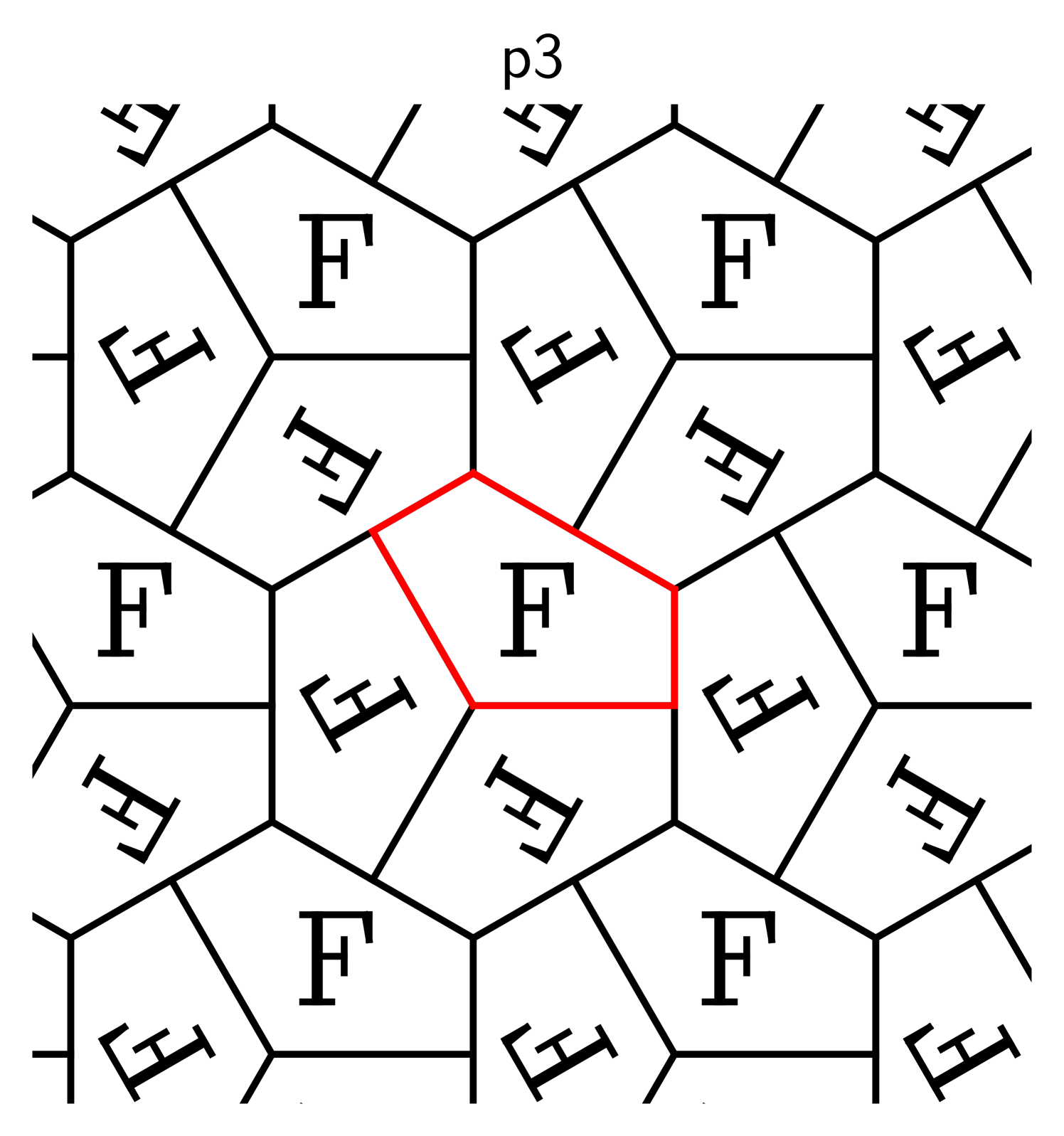
If we choose as the square and as the group of discrete horizontal and vertical shifts—that is, the two-dimensional analogue of the example above—we recover the two-dimensional Fourier transform. The function is constant; the functions are shown in Figure 4. If the group also contains other transformations, the basis looks less familiar. These are the basis functions for a group (p3) containing shifts and rotations of order three:
![[Uncaptioned image]](https://cdn.awesomepapers.org/papers/93546b17-f8fc-4a34-8d61-91c93d37517e/x10.png)
![[Uncaptioned image]](https://cdn.awesomepapers.org/papers/93546b17-f8fc-4a34-8d61-91c93d37517e/x11.png)
![[Uncaptioned image]](https://cdn.awesomepapers.org/papers/93546b17-f8fc-4a34-8d61-91c93d37517e/x12.png)
![[Uncaptioned image]](https://cdn.awesomepapers.org/papers/93546b17-f8fc-4a34-8d61-91c93d37517e/x13.png)
![[Uncaptioned image]](https://cdn.awesomepapers.org/papers/93546b17-f8fc-4a34-8d61-91c93d37517e/x14.png)
The same idea applies in any finite dimension . For , the can be visualized as contour plots. For instance, the first five non-constant basis elements for a specific three-dimensional group, designated I41 by crystallographers, look like this:
![[Uncaptioned image]](https://cdn.awesomepapers.org/papers/93546b17-f8fc-4a34-8d61-91c93d37517e/x15.png)
![[Uncaptioned image]](https://cdn.awesomepapers.org/papers/93546b17-f8fc-4a34-8d61-91c93d37517e/x16.png)
![[Uncaptioned image]](https://cdn.awesomepapers.org/papers/93546b17-f8fc-4a34-8d61-91c93d37517e/x17.png)
![[Uncaptioned image]](https://cdn.awesomepapers.org/papers/93546b17-f8fc-4a34-8d61-91c93d37517e/x18.png)
![[Uncaptioned image]](https://cdn.awesomepapers.org/papers/93546b17-f8fc-4a34-8d61-91c93d37517e/x19.png)
Our results show that any continuous invariant function can be represented
by a series expansion in functions . As for the Fourier transform, the functions form a orthonormal
basis of the relevant space. The functions can hence be seen as a generalization of the
Fourier transform from pure shift groups to crystallographic groups. All of this is made precise in Section 5.
Nonlinear representations: Factoring through an orbifold.
The second representation, in Section 6, generalizes an idea of David MacKay [45], who constructs periodic
functions on the line as follows: Start with a continuous function .
Choose a circle of circumference in , and restrict to the circle. The restriction is still
continuous. Now “cut and unfold the circle with on it” to obtain a function on the unit interval.
Since this function takes the same value at both interval boundaries, replicating it by shifts of integer length
defines a function on that is periodic and continuous:
More formally, MacKay’s approach constructs a function such that
We show how to generalize this construction to any finite dimension , any crystallographic group on , and any convex polytope with which tiles the space: For each and , there is a continuous, surjective map
| (2) |
such that
This is Theorem 15. Section 6.1 shows how to compute a representation of using multidimensional scaling.
The set can be thought of as an -dimensional surface in a higher-dimensional space . If contains only shifts, this surface is completely smooth, and hence a manifold. That is the case in MacKay’s construction, where is the circle, and the group p1 on , for which is the torus shown on the left:
For most crystallographic groups, is not a manifold, but
rather a more general object called an orbifold. The precise definition (see Appendix C) is somewhat technical, but
loosely speaking, an orbifold is a surface that resembles a manifold almost everywhere, except at a small number of
points at which it is not smooth.
That is illustrated by the orbifold on the right, which represents a group containing rotations, and has several “sharp corners”.
Applications I: Neural networks.
We can now define -invariant models by factoring through .
To define an invariant
neural network, for example, start with a continuous neural network with weight vector and some
output space . Then is a continuous and invariant neural network .
Here are examples for three groups (cm, p4, and p4gm) on , with three hidden layers and randomly generated weights:
Applications II: Invariant kernels. We can similarly define -invariant reproducing kernels on , by starting with a kernel on and defining a function on as
This function is again a kernel. In Section 7, we
show that its reproducing kernel Hilbert space consists of continuous -invariant
functions on .
We also show that, even though is not compact, behaves essentially like a kernel on a
compact domain (Proposition 23). In particular,
it satisfies a Mercer representation and a compact embedding property, both of which usually require
compactness. This behavior is specific to kernels invariant under crystallographic groups, and
does not extend to more general groups of isometries on .
Applications III: Invariant Gaussian processes.
There are two ways in which a Gaussian process (GP) can be invariant under a group: A GP is a distribution on
functions, and we can either ask for each function it generates to be invariant, or only require that its distribution is
invariant (see Section 8 for definitions). The former implies the latter. Both types of processes can be constructed
by factoring through an orbifold:
Suppose we start with a kernel (a covariance function) and a real-valued function (the mean function),
both defined on . If we then generate a random function on as
the function is -invariant with probability 1. The following are examples of such random functions, rendered as contour plots with non-smooth colormaps.
If we instead generate as
the distribution of is -invariant. See Section 8.
Properties of the Laplace operator.
Section 9 studies differentials and Laplacians of crystallographically invariant functions
.
The results are then used in the proof of the Fourier representation.
Consider a vector field , i.e., a function . An example
of such a vector field is the gradient . Lemma 27 shows that
the gradient transforms under elements of as
Proposition 28 shows that, for any vector field that transforms in this way, the total flux through the boundary of the polytope vanishes,
We can combine this fact with a result from the theory of partial differential equations, the so-called Green identity, which decomposes the Laplacian on functions on as
29 makes the statement precise. Using the fact that the flux vanishes,
we can show that the correction term on vanishes, and from that deduce that the
Laplace operator on invariant functions is self-adjoint (Theorem 30).
That allows us to draw on
results from the spectral theory of self-adjoint operators to solve (1).
Background and reference results.
Since our methods draw on a number of different fields,
the appendix provides additional background on groups of isometries (App. A),
functional analysis (App. B), and orbifolds (App. C),
and spectral theory (App. D).
2 Preliminaries: Crystallographic groups
Throughout, we consider a Euclidean space , and write for Euclidean distance in dimensions. Euclidean volume (that is, Lebesgue measure on ) is denoted . As we work with both sets and their boundaries, we must carefully distinguish dimensions: The span of a set is the smallest affine subspace that contains it. We define the dimension and relative interior of as
The boundary of is the set . If has dimension , then denotes Euclidean volume in . For example: If is a closed line segment, then , and is the length of the line segment, whereas . Taking the relative interior removes the two endpoints, whereas interior of in is the empty set. (No such distinction is required for the closure , since is closed in if and only if it is closed in .)
2.1. Defining crystallographic groups
Consider a group of isometries of . (See Appendix A for a brief review of definitions.) Every isometry of is of the form
| (3) |
Let be a set. We say that tiles the space with if the image sets completely cover the space so that only their boundaries overlap:
Each set is a tile, and the collection is a tiling of .
By a convex polytope, we mean the convex hull of a finite set of points [70]. Let be an -dimensional convex polytope. The boundary consists of a finite number of -dimensional convex polytopes, called the facets of . Thus, if tiles with , only points on facets are contained in more than one tile.
Definition 1.
A crystallographic group is a group of isometries that tiles with an -dimensional convex polytope .
The polytope is then also called a fundamental region (in geometry) or an asymmetric unit (in materials science) for . This definition of crystallographic groups differs from those given in the literature, but we clarify in Section A.2 that it is equivalent.

2.2. Basic properties
Some properties of can be read right off the definition: Since tiles the entire space with a set of finite diameter, we must have . Since is -dimensional and convex, it contains an open metric ball of positive radius. Each tile contains a copy of this ball, and these copies do not overlap. It follows that
| (4) |
A group of isometries that satisfies (4) for some is called discrete, in contrast to groups which contain, e.g., continuous rotations. Discreteness implies is countable, but not all countable groups of isometries are discrete (the group of rational-valued shifts is a non-example). In summary, every crystallographic group is an infinite, discrete (and hence countable) subgroup of the Euclidean group on .
Suppose we choose one of the tilings in Figure 1, and rotate or shift the entire plane with the tiling on it. Informally speaking, that changes the tiling, but not the tiling mechanism, and it is natural to consider the two tilings isomorphic. More formally, two crystallographic groups and are isomorphic if there is an orientation-preserving, invertible, and affine (but not necessarily isometric) map such that , where .
Fact 2 ([62, 4.2.2]).
Up to isomorphy, there are only finitely many crystallographic groups on for each . Specifically, there 17 such groups for , and 230 for .
3 Preliminaries: Invariant functions
A function , with values in some set , is -invariant if it satisfies
It is -invariant if it is -invariant for all . We are specifically interested in -invariant functions that are continuous, and write
More generally, a function is -invariant in each argument if
| (5) |
3.1. Tiling with functions
To construct a -invariant function, we may start with a function on and “replicate it by tiling”. For that to be possible, must in turn be the restriction of a -invariant function to . It must then satisfy if both and are in . We hence define the relation
We note immediately that implies each point is also contained in an adjacent tile, so both must be on the boundary of . The requirement
| (6) |
is therefore a periodic boundary condition. If it holds, the function
| (7) |
is well-defined on , and is -invariant. Conversely, every -invariant function can be obtained this way (by choosing as the restriction ). Informally, (7) says that we stitch together function segments on tiles that are all copies of , and these segments overlap on the tile boundaries. The boundary condition ensures that wherever such overlaps occur, the segments have the same value, so that (7) produces no ambiguities. The special case of (6) for pure shift groups—where is the identity matrix for all —is known as a Born-von Karman boundary condition (e.g., Ashcroft and Mermin [7]).
3.2. Orbits and quotients
An alternative way to express invariance is as follows: A function is -invariant if and only if it is constant on each set of the form
The set is called the orbit of . We see immediately that each orbit of a crystallographic group is countably infinite, but locally finite: The definition of discreteness in (4) implies that every bounded subset of contains only finitely many points of each orbit. We also see that each point is in one and only one orbit, which means the orbits form a partition of . The assignment is hence a well-defined map
The orbit set is also called the quotient set or just the quotient of , and is called the quotient map (e.g., Bonahon [15]). Since the orbits are mutually disjoint, we can informally think of as collapsing each orbit into a single point, and is the set of such points.
Quotient spaces are abstract but useful tools for expressing invariance properties: For any function , we have
| (8) |
since each point of represents an orbit and is invariant iff it is constant on orbits. We can also use the quotient to express continuity, by equipping it with a topology that satisfies
| (9) |
There is exactly one such topology, called the quotient topology in the literature. Its definition can be made more concrete by metrizing it:
Fact 3 (see Bonahon [15], Theorem 7.7).
If is crystallographic, the function
is a valid metric on , and it metrizes the quotient topology. A subset is open if and only if its preimage is open in .
Since is discrete, the infimum in is a minimum. The distance of two orbits (considered as points in ) is hence the shortest Euclidean distance between points in these orbits (considered as sets in ), see Figure 2 (right). If and are points in the polytope , we have
Informally speaking, implements the periodic boundary condition (6). The metric space is also called the quotient space or orbit space of . A very important property of crystallographic groups is that they have compact quotient spaces:
Fact 4 ([65, Proposition 1.6]).
If a discrete group of isometries tiles with a set , the quotient space is homeomorphic to the quotient space . If is crystallographic and tiles with a convex polytope, then is compact.
3.3. Transversals and projections
Since orbit spaces are abstract objects, we can only work with them implicitly. One way to do so is by representing each orbit by one of its points in . A subset of that contains exactly one point of each orbit is called a transversal. In general, transversals can be exceedingly complex sets [9], but crystallographic groups always have simple transversals. Algorithm 2 in the next section constructs a transversal explicitly. In the following, we will always write to mean
Given such a transversal, we can define the projector as
| (10) |
If we think of each point in as a concrete representative of an element of , then is similarly a concrete representation of the quotient map , and we can translate the identities above accordingly: The projector is by definition -invariant, since we can write in (7) as . That shows
| (11) |
Although is not continuous as a function , continuity only fails at the boundary, and behaves like a continuous function when composed with :
Lemma 5.
Let be a continuous function with values in a topological space . If satisfies (6), then is a continuous -invariant function . It follows that
| (12) |
Since exists for any choice of and , and since it can be evaluated algorithmically, we have hence reduced the problem of constructing continuous invariant functions to the problem of finding functions that satisfy the periodic boundary condition (6).
4 Taking quotients algorithmically: Orbit graphs
To work with invariant functions computationally, we must approximate the quotient metric. We do so using a data structure that we call an orbit graph, in which two points are connected if their orbits are close to each other. More formally, any undirected graph is a metric space when equipped with path length as distance. The metric space defined by the graph below discretizes the metric space . To define , fix constants . A finite set is an -net in if each point lies within distance of ,
see e.g., Cooper et al. [23]. If is an -net in , we call the graph
an orbit graph for and .
4.1. Computing orbit graphs
Algorithmically, an orbit graph can be constructed as follows: Constructing an -net is a standard problem in computational geometry and can be solved efficiently (e.g., Haussler and Welzl [33]). Having done so, the problem we have to solve is:
Since is a polytope, its diameter
can also be evaluated computationally. By definition of , we have
That shows the minimum is always attained for a point on a tile that lies within distance of . The set of transformations that specify these tiles is
This set is always finite, since is discrete and the ball of radius is compact. We can hence evaluate the quotient metric as
which reduces the construction of to a finite search problem. In summary:
Algorithm 1 (Constructing the orbit graph).
| 1.) | Construct the -net . |
|---|---|
| 2.) | Find local group elements . |
| 3.) | For each pair , find . |
| 4.) | Add an edge between and if . |
The construction is illustrated in Figure 3.
4.2. Computing a transversal
Recall that the faces of a polytope are its vertices, edges, and so forth; the facets are the -dimensional faces. The polytope itself is also a face, of dimension . See [70] for a precise definition. Given and , we will call two faces and -equivalent if for some . Thus, if , its equivalence class is . If is a facet, it is equivalent to at most one distinct facet, so its equivalence class has one or two elements. The equivalence classes of lower-dimensional faces may be larger—if is p1 and a square, for example, all four vertices of are -equivalent.
Algorithm 2 (Constructing a transversal).
| 1) | Start with an exact tiling. Enumerate all faces of . |
|---|---|
| 2) | Sort faces into -equivalence classes. |
| 3) | Select one face from each class and take its relative interior. |
| 4) | Output the union of these relative interiors. |
Lemma 6.
The set constructed by Algorithm 2 is a transversal.
Proof.
The relative interiors of the faces of a convex polytope are mutually disjoint and their union is , so each point is on exactly one such relative interior. Let be the face with , and consider any . Since the tiling is exact, is either a face of or . If , the intersection cannot be empty, so is a face and hence -equivalent to . It follows that the interior of a face of intersect the orbit if and only if it is in the equivalence class of . Since we select exactly one element of this class, exactly one point of is contained in . ∎
4.3. Computing the projector
Since is crystallographic, it contains shifts in linearly independent directions, and these shifts hence specify a coordinate system of . More precisely: There are elements of that (1) are pure shifts (satisfy ), (2) are linearly independent, and (3) are the shortest such elements (in terms of the Euclidean norm of ). Up to a sign, each of these elements is uniquely determined. We refer to the vectors as the shift coordinate system of .
Algorithm 3 (Computing the projector).
| 1.) | Perform a basis change from the shift coordinates to the standard basis of . |
|---|---|
| 2.) | Set . |
| 3.) | Find such that . |
| 4.) | Apply the reverse change of basis from standard to shift coordinates. |
5 Linear representation: Invariant Fourier transforms
In this section, we obtain a basis representation for invariant functions: given a crystallographic group , we construct a sequence of -invariant functions on such that any -invariant continuous function can be represented as a (possibly infinite) linear combination . If is generated by orthogonal shifts, the functions are an -dimensional Fourier basis. Theorem 7 below obtains an analogous basis for each crystallographic group .
5.1. Representation theorem
For any open set , we define the Laplace operator on twice differentiable functions as
Now consider specifically functions . Fix some , and consider the constrained partial differential equation
| (13) | ||||||
Clearly, there is always a trivial solution, namely the constant function . If (13) has a non-trivial solution , we call this a -eigenfunction and a -eigenvalue of the linear operator . Denote the set of solutions by
Since is a solution, and any linear combination of solutions is again a solution, is a vector space, called the eigenspace of . Its dimension
is the multiplicity of .
Theorem 7 (Crystallographically invariant Fourier basis).
Let be a crystallographic group that tiles with a convex polytope . Then the constrained problem (13) has solutions for countably many distinct values of , and these values satisfy
Every solution function is infinitely often differentiable. There is a sequence of solutions whose restrictions to form an orthonormal basis of the the space , and satisfy
A function is -invariant and continuous if and only if
where the series converges in the supremum norm.
Proof.
See Appendix G. ∎
Remark 8.
The space contains no non-trivial -invariant functions, since for every
On the other hand, the restriction is in , and completely determines . That makes the natural -space in the context of crystallographic invariance, and is the reason why the restrictions are used in the theorem. Since is isometric to for all , it does not matter which tile we restrict to.
5.2. Relationship to Fourier series
The standard Fourier bases for periodic functions on can be obtained as the special cases of Theorem 7 for shift groups: Fix some edge width , and choose and as
For these groups, all eigenvalue multiplicities are for each . For , the group is p1 (see Figure 1). Its eigenfunctions are shown in Figure 4.
To clarify the relationship in more detail, consider the case : Since is a second derivative, the functions and satisfy
and are hence eigenfunctions of with eigenvalue . For this choice of and , the invariance constraint in (13) holds iff for every . That is true iff
The eigenspaces are therefore the two-dimensional vector spaces
Any continuous function that is -invariant (or, equivalently, -periodic) can be expanded as
| (14) |
In the notation of Theorem 7, the coefficients are and , and
Note that the unconstrained equation has solutions for all in the uncountable set . The invariance constraint limits possible values to the countable set . If was continuous but not invariant, the expansion (14) would hence require an integral on the right. Since is invariant, a series suffices.
Remark 9 (Multiplicities and real versus complex coefficients).
Fourier series, in particular in one dimension, are often written using complex-valued functions as
Since Euler’s formula shows
that is equivalent to (14). The complex plane is not inherent to the Fourier representation, but rather a convenient way to parameterize the two-dimensional eigenspace . For general crystallographic groups, the complex representation is less useful, since the multiplicities may not be even, as can be seen in Figure 5.
5.3. Spectral algorithms
The eigenfunctions in Theorem 7 can be approximated by eigenvectors of a suitable graph Laplacian of the orbit graph as follows. We first compute an orbit graph as described in Section 4. We weight each edge of the graph by
| (15) |
The normalized Laplacian of the weighted graph is
| (16) |
and is the diagonal matrix containing the sum of each row of . See e.g., Chung [20] for more on the matrix . Our estimates of the eigenvalues and -functions of are the eigenvalues and eigenvectors of ,
These approximate the spectrum of in the sense that
see Singer [56]. Once an eigenvector is computed, values of at points can be estimated using standard interpolation methods.
Algorithm 4 (Computing Fourier basis).
| 1.) | Construct the orbit graph . |
|---|---|
| 2.) | Compute the normalized Laplacian matrix according to (16). |
| 3.) | Compute eigenvectors and eigenvalues of . |
| 4.) | Return eigenvalues and interpolated eigenfunctions. |
Alternatively, the basis can be computed using a Galerkin approach, which is described in Section 9.5. The functions in Figures 4, 5 and 6 are computed using the Galerkin method.
Remark 10 (Reflections and Neumann boundary conditions).
The orbit graph automatically enforces the boundary condition (6), since it measures distance in terms of .
The exception are group elements that are reflections, since these imply an additional property that the graph does not resolve:
If is a reflection over a facet , a point on (and hence ), and a -invariant smooth function,
we must have , and hence on . In the parlance of PDEs, this is a Neumann boundary condition,
and can be enforced in several ways:
1) For each point that is on , add a point to and
the edge to . Then constrain each eigenvector in Algorithm 4 to satisfy .
This approach is common in spectral graph theory (e.g., Chung [20]).
2) Alternatively, one may symmetrize the orbit graph: For vertext that is close to , add its reflection to
. Now construct the edge set according to using the augmented vertex set, and again constrain eigenvectors to
satisfy .
Either constrained eigenvalue problem can be solved using techniques of Golub [29].
6 Nonlinear representation: Factoring through an orbifold
We now generalize MacKay’s construction, as sketched in the introduction, from shifts to crystallographic groups. The construction defines a map
In MacKay’s case, is an interval and a circle. The circle can be obtained from by “gluing” the ends of the interval to each other. To generalize this idea, we proceed as follows: Starting with the polytope , we find any pair of points and on the same orbit of , and “bend” so that we can glue to . That results in a surface in , where since we have bent . If we denote the point on that corresponds to by , we obtain the maps above. We first show how to implement this construction numerically, and then consider its mathematical properties. In mathematical terms, the surface is an orbifold, a concept that generalizes the notion of a manifold. The term -orbifold is made precise in in Appendix C, but can be read throughout this section as a surface in that is “smooth almost everywhere”.
6.1. Gluing algorithms
The gluing algorithm constructs numerical approximations of and of . Here, is a surface in dimensions, where (as we explain below) may be larger than . As in the linear formulation of Section 5, we start with the orbit graph , but in this case weight the edges to obtain a weighted graph
The weighted graph provides approximate distances in quotient space. The surface is constructed from this graph by multidimensional scaling (MDS) [40]. MDS proceeds as follows: Let be the matrix of squared geodesic distances, with entries
Let be the eigenvalues and the eigenvectors of the matrix
The embedding of each point in the -net is then given by
The dimension is chosen to minimize error in the distances. From , the surface and the map are obtained by interpolation.
Algorithm 5 (Gluing with multidimensional scaling).
| 1.) | Construct the weighted orbit graph . |
|---|---|
| 2.) | Compute the eigenvalues and eigenvectors of . |
| 3.) | Compute vertex embeddings . |
| 4.) | Return interpolated vertex embeddings. |
Once can be computed, we can also compute , since the projector can be evaluated using Algorithm 3.
Remark 11.
The procedure satisfies two desiderata for constructing the orbifold map: 1) facets to be glued will be brought together, and 2) distances between interior points in will be approximately preserved. The embedding is unique up to isometric transformations. The embedding step is similar to the Isomap [61] algorithm, but unlike Isomap embeds into a higher-dimensional space rather than a lower-dimensional one.
6.2. Example: Invariant neural networks
Given and , compute and using Algorithm 5. Choose a neural network
Then is a real-valued neural network on . Figure 10 shows examples of for , where has three hidden layers of ten units each, with rectified linear (relu) activations, although the input dimension may vary according to the choice of and . The parameter vector is generated at random.
Remark 12.
Since most ways of performing interpolation in the construction of are amenable to automatic differentiation tools, this representation is easy to incorporate into machine learning pipelines. Moreover, universality results for neural networks (e.g., Hornik et al. [35]) carry over: If a class of neural networks approximates to arbitrary precision in , the the resulting functions approximate to arbitrary precision in (though the approximation rate may change under composition with ). See Corollary 17.
6.3. Exact tilings
Although the properties of general orbifolds constitute one of the more demanding problems of modern mathematics, orbifolds of crystallographic groups are particularly well-behaved, and are well-understood. That we can draw directly on this theory is due to the fact that it uses a notion of gluing very similar to that employed by our algorithms as a proof technique [15, 53]. The two notions align under an additional condition: A convex polytope is exact for if tiles with , and if each face of can be represented as
Not every with which tiles is exact—in Figure 1, for example, the polytopes shown for pg and p3 are not exact, though all others are. However, given and , we can always construct an exact surrogate as follows: Choose any point that is not a fixed point for any . If is crystallographic, that is true for every point in the interior of . For each , the set
is a half-space in (see Figure 11/left). The intersection
of these half-spaces is called a Dirichlet domain for (Figure 11/right).
Fact 13 ([53, 6.7.4]).
If is crystallographic, is an exact convex polytope for .
Example 14.
For illustration, consider the group pg: We start with a rectangle . The group is generated by two glide reflections and , each of which shifts horizontally and then reflects it about one of its long edges (Figure 12/left). Exactness fails because the set , marked in black, is not a complete edge of . A Dirichlet domain for this tiling differs significantly from (Figure 12/right). Although substituting for changes the look of the tiling, it does not change the group—that is, we still work with the same set of transformations (rather than another group in the same isomorphism class), and the axes of reflections are still defined by the faces of rather than those of .
6.4. Properties of embeddings
Algorithm 5 can be interpreted as computing a numerical approximation
to a “true” embedding map , namely the map in (2) in the introduction.
Our main result on the nonlinear representation, Theorem 15 below,
shows that this map indeed exists for every crystallographic group, and describes some of
its properties. The proof of the theorem shows that and the set can be constructed
by the following abstract gluing algorithm.
Abstract gluing construction.
1.)
Glue: Identify each with the unique point satisfying .
2.)
Equip the glued set with metric .
3.)
Embed the metric space as a subset for some .
4.)
For each , define as the representative of on .
5.)
Set .
Since contains at least one point of each orbit, and the gluing step identifies all points identifies all points on the same orbit with each other, the glued set can be regarded as the quotient set . Recall that an embedding is a map that is a homeomorphism (a continuous bijection with continuous inverse) of the metric spaces and .
The state the theorem, we need one additional bit of terminology: The stabilizer of in is the set of all that leave invariant,
see Vinberg and Shvartsman [65], Ratcliffe [53], Bonahon [15]. We explain the role of the stabilizer in more detail in the next subsection.
Theorem 15.
Let be a crystallographic group that tiles with an exact convex polytope . Then the set constructed by gluing is a compact -orbifold that is isometric to . This orbifold can be embedded into for some
that is, there is compact subset such that the metric space is homeomorphic to . In particular, every point is represented by one and only one point . We can hence define a map
The map is continuous, surjective, and -invariant. A function , with values in some topological space , is -invariant and continuous if and only if
is smooth almost everywhere, in the sense that
where denotes the open Euclidean metric ball of radius centered at .
Proof.
See Appendix H. ∎
Remark 16.
(a) Note carefully what the theorem does and does not show about the
embedding algorithm in Section 6.1: It does say that the
glued set constructed by the algorithm discretizes an orbifold, and that an -dimensional
embedding of this orbifold exists. It does
not show that the embedding computed by MDS matches this dimension—indeed, since
MDS attempts to construct an embedding that is also isometric (rather than just homeomorphic), we
must in general expect the MDS embedding dimension to be larger, and we have at present no proof
that an isometric embedding always exists.
(b) If the tiling defined by and is not exact,
we can nonetheless define an embedding that represents continuous functions that are invariant
functions with respect to this tiling: Construct a Dirichlet domain , and then construct by applying the gluing
algorithm to . Functions constructed as are then invariant for the tiling .
We have now seen different representations of continuous -invariant functions on , respectively by continuous functions on , on the abstract space , and on . On , we must explicitly impose the periodic boundary condition, so we are using the set
In these representations, the projector , the quotient map , and the embedding map play very similar roles. We can make that observation more rigorous:
Corollary 17.
Given a crystallographic group that tiles with a convex polytope , consider the maps
| and | and | ||||||||
where is only defined if is exact. Equip all spaces with the supremum norm. Then and are isometric isomorphisms, and if is exact, so is . In particular, is always a separable Banach space.
Proof.
By Lemma 5, (8) and Theorem 15, all three maps are bijections. We also have
and the same holds mutatis mutandis on and , so all maps are isometries. Since is compact, is separable [3, 3.99]. The same hence holds for the closed subspace , and by isometry for . ∎
6.5. Why the glued surface may not be smooth
Whether or not the glued surface is smooth depends on whether the transformations in leave any points invariant. It is a known fact in geometry (and made precise in the proof of Theorem 15) that
| glued surface is a manifold | ||||
| That can be phrased in terms of the stabilizer as | ||||
| glued surface is a manifold | ||||
It is straightforward to check that is a group [65]. Since each is an isometry, and shifts of have no fixed points, can only hold if . Thus, is always a subset of the point group (in the terminology of Appendix A), which means it is finite. To illustrate its effect on the surface, consider the following examples.
Example 18.
(a) Recall that MacKay’s construction [45], as sketched in the introduction,
can be translated to crystallographic groups by setting and choosing as shifts. In this case,
for each , and the glued surface is a circle, which is indeed a manifold.
The two-dimensional analogue is to choose and as the group p1 in Figure 1,
in which case the glued surface is a torus as shown in Figure 9, and hence again a manifold.
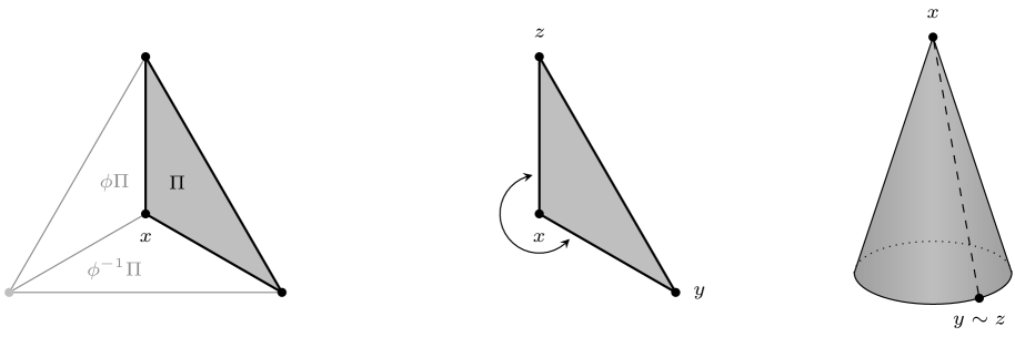
(b) Now suppose is a triangle, one of its corners, and a rotation
around , as illustrated in Figure 13. Then , and the glued surface is a cone with as its tip.
That means is not a manifold, because no neighborhood of the tip can be mapped isometrically to a neighborhood in .
7 Invariant kernels
Throughout this section, is a kernel, i.e., a positive definite function, and is its reproducing kernel Hilbert space, or RKHS. Appendix B reviews definitions. We consider kernels that are -invariant in both arguments in the sense of (5), that is,
That is the natural notion of invariance for most purposes, since such kernels are precisely those that define spaces of -invariant functions:
Proposition 19.
If and only if is -invariant in each argument, all functions are -invariant. If is also continuous, all are continuous, and hence .
Theorem 15 implies that, to define an invariant kernel, we can start with any kernel on the embedding space , and compose it with the embedding map :
Corollary 20.
Let be a kernel on . Then the function
is a kernel on that is -invariant in both arguments. If is continuous, so is .
That follows immediately from Theorem 15 and the fact that the restriction of a kernel to a subset is again a kernel [59].
Example 21.
Suppose is an radial basis function (RBF) kernel with length scale on , and hence of the form . Then is simply
Figure 14 illustrates this kernel the two-dimensional groups pg and p4gm and the three-dimensional groups I4 and P6/m.
Once we have constructed an invariant kernel, its application to machine learning problems is straightforward. That becomes obvious if we define , often called the feature map of [59]. Using the definition of the scalar product on and the reproducing property (see Section B.4), we then have
If is -invariant, then is also -invariant by construction. Recall that most kernel methods in machine learning are derived by substituting a Euclidean scalar product by , thereby making a linear method nonlinear. Using a -invariant kernel results in a -invariant method.
Example 22 (Invariant SVM).
A support vector machine (SVM) with kernel is determined by two finite sets of points and in . To train the SVM, one maps these points into via , finds the shortest connecting line between the convex hulls of and , and determines a hyperplane that is orthogonal to this line and intersects its center—equivalently, in dual formulation, the unique hyperplane that separates the convex hulls of and and maximizes the -norm distance to both. The set of points in whose image lies on is the decision surface of the SVM in . The hyperplane can be specified by two functions (an offset vector) and (a normal vector) in : A function lies on if and only if
Let be a point in . If and are points with and , then
Since invariance of implies , that shows the decision surface is -invariant. Figure 15 shows examples. In these figures the data were randomly generated with regions assigned labels using a random function generated as in Section 8. The support vectors are highlighted and illustrate the effects of symmetry constraints: the decision surface can be determined by data observed far away.
Two of the most important results on kernels are Mercer’s theorem and the compact inclusion theorem [59, Chapter 4]. The latter shows the inclusion map is compact, and is used in turn to establish good statistical properties of kernel methods, such as oracle inequalities and finite covering numbers [59]. Both results assume that has compact support. If is invariant under a crystallographic group, its support is necessarily non-compact, but the next result shows that versions of both theorems hold nonetheless:
Proposition 23.
If is continuous and -invariant in both arguments, the inclusion map is compact. There exist functions and scalars such that
and the scaled sequence is an orthonormal basis of . With this basis,
where each series converges in and hence (by compactness of inclusion) also uniformly.
Intuitively, that is the case because every -invariant kernel is the pullback of a kernel on , and is compact. Figure 15 shows an application of such a kernel to generate a two-class classifier with an -invariant decision surface.
8 Invariant Gaussian processes
We now consider the problem of generating random functions such that each instance of is continuous and -invariant with probability 1. That can be done linearly using the generalized Fourier representation, by generating the coefficients in Theorem 7 at random. Here, we consider the nonlinear representation instead: If we set
Theorem 15 implies that is indeed continuous and -invariant with probability , and hence a random element of . Conversely, the result also implies that every random element of is of this form, for some random element of .
8.1. Almost surely invariant processes
Recall that a random function is a Gaussian process if the joint distribution of the random vector is Gaussian for any finite set of points . The mean and covariance function of a Gaussian process are defined as
The covariance function is always positive definite, and hence a kernel on . The distribution of a Gaussian process is completely determined by and , and conditions for to satisfy continuity or stronger regularity conditions can be formulated in terms of . See e.g., Marcus and Rosen [46] for more background.
Proposition 24.
Let be a continuous Gaussian process on , with mean and covariance function . Then is a continuous random function on , and is -invariant with probability 1. Consider any finite set of points
Then is a Gaussian random vector, with mean and covariance
Clearly, cannot be a Gaussian process on : Since is invariant, completely determines , so cannot be jointly Gaussian. Put differently, conditioning on its values on renders non-random. Loosely speaking, the proposition hence says that is “as Gaussian” as a -invariant random function can be. Figure 16 illustrates random functions generated by such a process.
Example 25.
The construction of MacKay [45] described in the introduction was designed specifically for Gaussian processes, to generate periodic functions at random. We can now generalize these processes from periodicity to crystallographic invariance: Given and , construct the embedding map . Choose as the RBF kernel (21) on , and as the constant function on . Then generate as
For visualization, draws can be approximated by the randomized feature scheme of Rahimi and Recht [51]. Figure 16 shows examples for chosen as p2 and p31m on , and for P-6 and P422 on .
8.2. Distributionally invariant processes
Another type of invariance that random functions can satisfy is distributional -invariance, which holds if
Here, denotes equality in distribution. That is equivalent to requiring that the distribution of satisfies for every measurable set . For crystallographic groups, distributionally invariant Gaussian processes can be constructed by factoring the parameters, rather than the random function , through the embedding in Theorem 15:
Corollary 26.
Let be a real-valued function and a kernel on . If is the Gaussian process on with mean and covariance function , then is distributionally -invariant, i.e. for all .
Almost sure invariance implies distributional invariance; distributional invariance is typically a much weaker property. Frequently encountered examples of distributional invariance are all forms of stationarity (distributional invariance under shift groups) and of exchangeability (permutation groups).
9 The Laplace operator on invariant functions
The results in this section describe the behavior of the Laplace operator on -invariant functions. All of these are ingredients in the proof of the Fourier representation. We first describe the transformation behavior of differentials of invariant functions, in Section 9.1. Gradients turn out to be invariant under shifts and equivariant under orthogonal transformations. Gradient vector fields, and more generally vector fields with the same transformation behavior as gradients, have a cancellation property—their integral orthogonal to the tile boundary vanishes (Section 9.2). We then define the relevant solution space for the spectral problem, which has Hilbert space structure (so that we can define orthogonality and self-adjointness) but has smoother elements than , in Section 9.3. Once the Laplacian has been properly defined on this space, we can use the cancellation property to show it is self-adjoint.
9.1. Differentials and gradients of invariant functions
Given a differentiable function , denote the differential at as
The next result summarizes how invariance of under a transformation affects . Note the order of operations matters: is the differential of the function , whereas transforms the differential of by .
Lemma 27.
If is invariant under an isometry and differentiable, then
| (17) |
If in particular , the gradient satisfies
| (18) |
The Hessian matrix and the Laplacian satisfy
| (19) |
Proof.
Since is affine, its differential is constant. The chain rule shows
By invariance, and are the same function, and hence . Substituting into the identity above shows (17), since . For , the transpose is the gradient, and (17) becomes (18). Using (18), the Hessian can be written as
Another application of the chain rule then shows
which is the first statement in (19). Since the Laplacian is the trace of , and the trace in invariant under change of basis, that implies
9.2. Flux through the tile boundary
The next result is the key tool we use to prove self-adjointness of the Laplacian. We have seen above that the gradient of a -invariant function transforms under according to (18). We now abstract from the specific function , and consider any vector field that transforms like the gradient on the tile boundary, i.e.
| (20) |
For a polytope with facets , we define the normal field on the boundary as
where is the unit normal vector of the facet , directed outward with respect to . In vector analysis, the projection of a vector field onto the direction orthogonal to is known as the flux of through the boundary.
Proposition 28 (Flux).
Let be a crystallographic group that tiles with a convex polytope . If a vector field is integrable on and satisfies (20), then
Proof.
See Appendix E. ∎
9.3. The Sobolev space of invariant functions
The proof of Theorem 7 follows a well-established strategy in spectral theory: The relevant spectral results hold for self-adjoint operators, and self-adjointness can only be defined with respect to an inner product. Since the space on which the Laplace operator is defined is a Banach space, but has no inner product, one must hence first embed the problem into a suitable Hilbert space. For the Laplacian, this is generally a first-order Sobolev space; see Appendix B for a review of definitions, and Brezis [19], Maz’ya [47], McLean [48] for more on spectral theory and the general approach.
In our case, we proceed as follows: Since invariant functions are completely determined by their values on , we can equivalently solve the problem on the bounded domain rather than the unbounded domain . That gives us access to a number of results specific to bounded domains. We also observe that the invariance constraint is a linear constraint—if two functions satisfy it, so do their linear combinations—so the feasible set of this constraint is a vector space, and we can encode the constraint by restriction to a suitable subspace. We start with the vector space
| (21) |
The elements of are hence infinitely often differentiable on , and their continuous extensions to the closure satisfy the periodic boundary condition (6). We then define the Sobolev space of candidate solutions as
equipped with the norm and inner product of . As a closed subspace of a Hilbert space, it is a Hilbert space.
9.4. The Laplace operator on
We now have to extend to all elements of . In general, a linear operator on a closed subspace is an extension of to if it satisfies
| (22) |
The extended operator is self-adjoint on if
To prove self-adjointness, one decomposes as
This is the Green identity alluded to in the introduction. To make it precise, we need two quantities: One is the energy form or energy product
| (23) |
Since it only involves first derivatives, and both appear under the integral, it is well-defined for any , and is hence a symmetric bilinear form . It is positive definite, since
| (24) |
Substituting the definition of into that of the scalar product in (B.6) shows that
| (25) |
The second quantity is the conormal derivative
The precise statement of the decomposition above is then as follows.
Fact 29 (Green’s identity).
If the domain is sufficiently regular—in particular, if is a convex polytope—then
Informally, this shows that “behaves self-adjointly” in the interior of , where derivatives can be computed in all directions around a point. At points on , the boundary truncates derivatives in some direction, and that requires a correction term .
Theorem 30 (Properties of the Laplacian).
Let be a crystallographic group that tiles with a convex polytope . Then has a unique extension to a linear operator on . This operator is self-adjoint and continuous on , and satisfies
| (26) |
for all .
The proof uses the flux property to show that crystallographic symmetry makes the boundary term cancel. Since is symmetric, that makes self-adjoint. In the parlance of elliptic differential equations, (26ii) says that is coercive on (see [48]).
Proof.
See Appendix F. ∎
9.5. Linear representations from a nonlinear ansatz
The properties of Laplace operators lead naturally to a class of numerical approximations known as Galerkin methods (e.g., Braess [18]). Using the embedding map , we can derive a Galerkin method that can be used to compute the Fourier basis functions in Theorem 7—that is, we can use the nonlinear representation approach in the numerical approximation of the linear representation. The Galerkin method can be more accurate than the spectral approach in Algorithm 4, and was used to render Figures 4, 5 and 6.
Galerkin methods posit basis functions and approximate an infinite dimensional function space by the finite-dimensional subspace . In our case, we approximate solutions of (13) by approximating their restrictions . We hence need functions . W we start with functions , and set . We then assume of (13) is in the span, and hence of the form
| (27) |
If solves the eigenvalue problem (13), satisfies
Applying (26) and substituting in (27) shows
If we define matrices with entries and , that becomes
The entries of and can be computed with off-the-shelf cubature methods, and we can then solve for the pair .
Remark 31.
(a) If and the basis functions are implemented with JAX [17] or a similar
automatic differentiation tool, the gradients in (23) are available, which avoids finite
difference approximation and explicit computation of second derivatives.
(b) Neumann boundary conditions for reflections (see Remark 10) can be
enforced using the methods of Golub [29].
(c) The basis functions can be almost any basis on .
Figures 4–6 were rendered by placing points uniformly on ,
and centering radial basis functions at the points in .
10 Related work and additional references
In machine learning.
There has been substantial work on group invariance and equivariance in machine learning, with a focus on finite and compact groups.
Most salient has been work on approximate translation invariance and equivariance in convolutional neural networks for images [44, 39] and speech [1], although this work has not been framed in a group-theoretic way.
To our knowledge the earliest explicit consideration of compact and finite group structure in machine learning was from a Fourier perspective by Kondor [38]; this was primarily in the context of Hilbert-space formalisms of learning.
The current perspective on compact and finite group equivariance in deep learning arose largely from Cohen and Welling [21].
There has been widespread application of machine learning models when group invariance or equivariance is desired, e.g., permutation invariance for sets [69] and equivariance for neural auction design [52].
In the natural sciences, rotation invariance has been used for astronomy [25] and equivariance has proved important for molecular applications [8].
Permutation equivariance of transformer architectures plays a crucial role in large language model [64].
In crystallography.
Crystallographers have completely described the 17 two-dimensional and 230 three-dimensional
crystallgraphic groups and various tilings they describe,
and tabulated many of their properties [31].
The emphasis in this work differs somewhat from that in mathematics—in particular,
work in crystallography emphasizes polytopes that occur in crystal structures
(and which are not necessarily exact in the terminology used in Theorem 15),
whereas more abstract work in geometry tends to work with Dirichlet domains or other exact tilings.
A long line of work in the context of X-ray crystallography modifies the matrices
that occur in fast Fourier transforms (FFTs) to speed up computation if a crystallographic symmetry
is present in the data. This starts with the work of
Bienenstock and Ewald [13] and Ten Eyck [60], see also An et al. [5].
The introduction of Seguel and Burbano [55] gives an overview.
This work does not attempt to derive invariant Fourier bases.
In Fourier and PDE analysis.
As we have already explained in some detail, the special case of Theorem 7
for and yields
the Fourier transform. For this problem, the periodic boundary condition can be
replaced by a Neumann condition, and spectral problems with Neumann conditions
are standard material in textbooks [19, 43].
For shifts that are not axis-parallel, the
periodic boundary condition is known
as a Born-von Karman boundary condition [7]. We are not aware of
extensions to crystallographic groups.
An introduction to the PDE techniques used in our proofs
can be found in Brezis [19]. The conditions imposed there are too restrictive
for our problems, however; a treatment general enough to cover all results we use
is given by McLean [48].
In geometry.
Thurston [e.g., 62] coined the term orbifold in the
1970s. Commonly cited references include Scott [54], Bonahon and Siebenmann [16], Thurston [62];
Apanasov [6] has a detailed bibliography.
These all focus on general groups, however, for which the theory is much harder than in our case.
The quotient space structure of crystallographic groups was already understood much earlier
by the Göttingen and Moscow schools [65].
A readable introduction to isometry groups and their quotients is given by Bonahon [15].
The comprehensive account of Ratcliffe [53] is
more demanding, but covers all results needed in our proofs.
Vinberg and Shvartsman [65] cover the
geometric aspects of crystallographic groups. Conway, Burgiel, and
Goodman-Strauss [22]
explain the geometry of orbifolds heuristically, with many illustrations.
11 Some open problems
Our approach raises a range of further questions well beyond the scope of the present paper,
including in particular those concerning numerical and statistical accuracy. We briefly
discuss some aspects of this problem.
Linear representation.
Suppose we represent a -invariant continuous function
by evaluating the generalized Fourier basis in Theorem 7
using the spectral algorithm in Section 5.3.
The algorithm returns numerical approximations of the
basis functions. We may then expand as
There are three principal sources of error in this representation:
-
1.
The truncation error, since is finite.
-
2.
Any error incurred in computation of the coefficients .
-
3.
The error incurred by approximating the actual basis functions by .
The truncation error (1) concerns the question how well the vector space approximates the space or . This problem is studied in approximation theory. Depending on the context, one may choose the first basis vectors (a strategy called “linear approximation” in approximation theory), or greedily choose those basis vectors that minimize some error measure (“nonlinear approximation”), see DeVore [24]. Problem (2) depends on the function , and on how it is represented computationally. If must itself be reconstructed from samples, the coefficients are themselves estimators and incur statistical errors.
The error immediately related to our method is (3), and for the method of Section 5 depends on how well the graph Laplacian used in Section 5.3 approximates the Laplacian . This problem has been studied in a number of fields, including machine learning in the context of dimensionality reduction [10] and numerical mathematics in the context of homogenous Helmholtz equations [32], and is the subject of a rich literature [41, 11, 56, 34, 27, 28]. Available results show that, as in the -net, the matrix converges to , where the approximation can be measures in different notions of convergence, in particular pointwise and spectral convergence. The cited results all concern the manifold case. We are not aware of similar results for orbifolds.
For the method of Section 9.5, the error depends largely on the choice of basis in and the accuracy of the numerical integrals, as well as the orbifold map approximation itself (see below).
Error analysis of the Rayleigh-Ritz method has a long history, see, e.g., Weinberger [66], Wendroff [68], Weinberger [67].
Nonlinear representation.
If we define a -invariant statistical or machine learning model on by factoring it through an
orbifold, one may ask approximation questions of a more statistical flavor:
Suppose we define a class of functions
on the embedding space , with some parameter space .
We then define a class of -invariant functions on as
Depending on the context, we may think of the functions e.g., as neural networks or regressors. The task is then to conduct inference, i.e., to compute a point estimate of (say by maximum likelihood estimation or empirical risk minimization), or to compute a posterior on in a Bayesian setup. Since and share the same parameter space, any such inference task can be “pushed forward” forward to the embedding space, that is,
The error can again be separated into components:
-
1.
The statistical error associated with fitting .
-
2.
The “forward distortion” introduced by the map .
-
3.
The “backward distortion” introduced by the map .
Problem (1) reduces to the statistical properties of , and depends on both the model and the chosen inference method. Problem (2) and (3), however, raise a number of new questions: The map is, by Theorem 15, bijective (which means it does not introduce identifiability problems) and continuous. As the proof of Proposition 23 shows, it also preserves density properties of certain function spaces, which can be thought of as a qualitative approximation result. Quantitative results are different matter: To bound the effect of transformations on statistical errors typically requires a stronger property than continuity, such as differentiability or at least a Lipschitz property. In results on manifold learning, the curvature of often plays an explicit role. Orbifolds introduce a further challenge, since smoothness properties fail at the tips and edges introduced by points with non-trivial stabilizers. On the other hand, non-differentiabilities of crystallographic orbifolds have lower-bounded opening angles [62]—note the tip of the cone in Figure 13, for example, is not a cusp—so it may be possible to mitigate these problems.
Acknowledgements
The authors would like to thank Elif Ertekin and Eric Toberer for valuable discussions. RPA is supported in part by NSF grants IIS-2007278 and OAC-2118201. PO is supported by the Gatsby Charitable Foundation.
References
- Abdel-Hamid et al. [2014] O. Abdel-Hamid, A.-R. Mohamed, H. Jiang, L. Deng, G. Penn, and D. Yu. Convolutional neural networks for speech recognition. IEEE/ACM Trans. Audio Speech Lang. Process., 22:1533–1545, 2014.
- Adams and Fournier [2003] R. A. Adams and J. J. F. Fournier. Sobolev Spaces. Academic Press, 2003.
- Aliprantis and Border [2006] C. D. Aliprantis and K. C. Border. Infinite-Dimensional Analysis. Springer, 2006.
- Aliprantis and Burkinshaw [2006] C. D. Aliprantis and O. Burkinshaw. Positive Operators. Springer, 2006.
- An et al. [1990] M. An, J. W. Cooley, and R. Tolimieri. Factorization method for crystallographic Fourier transforms. Adv. Appl. Math, 11:358–371, 1990.
- Apanasov [2000] B. Apanasov. Conformal geometry of discrete groups and manifolds. de Gruyter, 2000.
- Ashcroft and Mermin [1976] N. W. Ashcroft and N. D. Mermin. Solid State Physics. Harcourt, 1976.
- Batzner et al. [2022] S. Batzner, A. Musaelian, L. Sun, M. Geiger, J. P. Mailoa, M. Kornbluth, N. Molinari, T. E. Smidt, and B. Kozinsky. E (3)-equivariant graph neural networks for data-efficient and accurate interatomic potentials. Nature Communications, 13(1):2453, 2022.
- Becker and Kechris [1996] H. Becker and A. S. Kechris. The descriptive set theory of Polish group actions. Cambridge Univ. Press, 1996.
- Belkin and Niyogi [2003] M. Belkin and P. Niyogi. Laplacian eigenmaps for dimensionality reduction and data representation. Neural Comput., 15(6):1373–1396, 2003.
- Belkin and Niyogi [2008] M. Belkin and P. Niyogi. Towards a theoretical foundation for Laplacian-based manifold methods. J. Comput. System Sci., 74(8):1289–1308, 2008.
- Bell [1954] D. G. Bell. Group theory and crystal lattices. Rev. of Modern Phys., 26(3):311, 1954.
- Bienenstock and Ewald [1962] A. Bienenstock and P. P. Ewald. Symmetry of Fourier space. Acta Cryst., 15:1253–1261, 1962.
- Bloem-Reddy and Teh [2020] B. Bloem-Reddy and Y. W. Teh. Probabilistic symmetries and invariant neural networks. J. Mach. Learn. Res., 21(90):1–61, 2020.
- Bonahon [2009] F. Bonahon. Low-Dimensional Geometry. Amer. Math. Soc., 2009.
- Bonahon and Siebenmann [1985] F. Bonahon and L. Siebenmann. Seifert orbifolds and their role as natural crystalline parts of arbitrary compact irreducible 3-orbifolds. In London Math. Soc. Lect. Notes, volume 95, pages 18–85. Cambridge Univ. Press, 1985.
- Bradbury et al. [2018] J. Bradbury, R. Frostig, P. Hawkins, M. J. Johnson, C. Leary, D. al Maclaurin, G. Necula, A. Paszke, J. VanderPlas, S. Wanderman-Milne, and Q. Zhang. JAX: composable transformations of Python+NumPy programs, 2018. URL http://github.com/google/jax.
- Braess [2007] D. Braess. Finite Elements. Springer, 2007.
- Brezis [2011] H. Brezis. Functional Analysis, Sobolev Spaces, and Partial Differential Equations. Springer, 2011.
- Chung [1997] F. Chung. Spectral graph theory. Amer. Math. Soc., 1997.
- Cohen and Welling [2016] T. Cohen and M. Welling. Group equivariant convolutional networks. In Int. Conf. Machine Learning, pages 2990–2999. PMLR, 2016.
- Conway et al. [2016] J. H. Conway, H. Burgiel, and C. Goodman-Strauss. The Symmetries of Things. CRC Press, 2016.
- Cooper et al. [2000] D. Cooper, C. D. Hodgson, and S. P. Kerckhoff. Three-dimensional Orbifolds and Cone-Manifolds. Math. Soc. Japan, 2000.
- DeVore [1998] R. A. DeVore. Nonlinear approximation. Acta Numer., pages 51–150, 1998.
- Dieleman et al. [2015] S. Dieleman, K. W. Willett, and J. Dambre. Rotation-invariant convolutional neural networks for galaxy morphology prediction. Monthly Not. Roy. Astronom. Soc., 450(2):1441–1459, 2015.
- Dresselhaus et al. [2007] M. S. Dresselhaus, G. Dresselhaus, and A. Jorio. Group theory: application to the physics of condensed matter. Springer, 2007.
- Dunson et al. [2021] D. B. Dunson, H.-T. Wu, and N. Wu. Spectral convergence of graph Laplacian and heat kernel reconstruction in from random samples. Appl. Comput. Harmon. Anal., 55:282–336, 2021.
- Garc´ıa Trillos et al. [2020] N. García Trillos, M. Gerlach, M. Hein, and D. Slepčev. Error estimates for spectral convergence of the graph Laplacian on random geometric graphs toward the Laplace–Beltrami operator. Found. Comput. Math., 20(4):827–887, 2020.
- Golub [1973] G. H. Golub. Some modified matrix eigenvalue problems. SIAM review, 15(2):318–334, 1973.
- Gruber [2007] P. M. Gruber. Convex and Discrete Geometry. Springer, 2007.
- Hahn [2011] T. Hahn. International tables for crystallography, volume A. Wiley, 2011.
- Harari and Turkel [1995] I. Harari and E. Turkel. Accurate finite difference methods for time-harmonic wave propagation. J. Comput. Phys., 119(2):252–270, 1995.
- Haussler and Welzl [1987] D. Haussler and E. Welzl. -nets and simplex range queries. Discrete Comput. Geom., 2(2):127–151, 1987.
- Hein et al. [2005] M. Hein, J.-Y. Audibert, and U. v. Luxburg. From graphs to manifolds–weak and strong pointwise consistency of graph Laplacians. In Proc. of COLT, pages 470–485, 2005.
- Hornik et al. [1989] K. Hornik, M. Stinchcombe, and H. White. Multilayer feedforward networks are universal approximators. Neural Networks, 2(5):359–366, 1989.
- Johnston [1960] D. Johnston. Group theory in solid state physics. Rep. Progr. Phys., 23(1):66, 1960.
- Killingbeck [1970] J. Killingbeck. Group theory and topology in solid state physics. Rep. Progr. Physics, 33(2):533, 1970.
- Kondor [2008] I. R. Kondor. Group Theoretical Methods in Machine Learning. PhD thesis, Columbia Univ., 2008.
- Krizhevsky et al. [2017] A. Krizhevsky, I. Sutskever, and G. E. Hinton. Imagenet classification with deep convolutional neural networks. Communications of the ACM, 60(6):84–90, 2017.
- Kruskal [1964] J. B. Kruskal. Multidimensional scaling by optimizing goodness of fit to a nonmetric hypothesis. Psychometrika, 29(1):1–27, 1964.
- Lafon [2004] S. Lafon. Diffusion maps and geometric harmonics. PhD thesis, Yale University, 2004.
- Lax [2001] M. Lax. Symmetry principles in solid state and molecular physics. Courier Corporation, 2001.
- Lax [2002] P. D. Lax. Functional Analysis. Wiley, 2002.
- LeCun et al. [1989] Y. LeCun, B. Boser, J. Denker, D. Henderson, R. Howard, W. Hubbard, and L. Jackel. Handwritten digit recognition with a back-propagation network. Adv. Neural Inf. Process. Systems, 2, 1989.
- MacKay [1998] D. J. C. MacKay. Introduction to Gaussian processes. NATO ASI Series F, 168:133–166, 1998.
- Marcus and Rosen [2006] M. B. Marcus and J. Rosen. Markov processes, Gaussian processes, and local times. Cambridge Univ. Press, 2006.
- Maz’ya [2011] V. Maz’ya. Sobolev Spaces. Springer, 2nd edition, 2011.
- McLean [2000] W. McLean. Strongly Elliptic Systems and Boundary Integral Equations. Cambridge Univ. Press, 2000.
- Munkres [2000] J. R. Munkres. Topology. Prentice Hall, 2nd edition, 2000.
- Pears [1975] A. R. Pears. Dimension theory of general spaces. Cambridge University Press, 1975.
- Rahimi and Recht [2007] A. Rahimi and B. Recht. Random features for large-scale kernel machines. Adv. Neural Inf. Process. Systems, 20, 2007.
- Rahme et al. [2021] J. Rahme, S. Jelassi, J. Bruna, and S. M. Weinberg. A permutation-equivariant neural network architecture for auction design. In Proc. AAAI, volume 35, pages 5664–5672, 2021.
- Ratcliffe [2006] J. G. Ratcliffe. Foundations of Hyperbolic Manifolds. Springer, 2nd edition, 2006.
- Scott [83] P. Scott. The geometries of -manifolds. Bull. London Math. Soc, 5:401–487, 83.
- Seguel and Burbano [2003] J. Seguel and D. Burbano. A scalable crystallographic FFT. In Lecture Notes in Comput. Sci., volume 2840, pages 134–141. Springer, 2003.
- Singer [2006] A. Singer. From graph to manifold Laplacian: The convergence rate. Appl. Comput. Harmon. Anal., 21(1):128–134, 2006.
- Slater [1965] J. Slater. Space groups and wave-function symmetry in crystals. Rev. Modern Phys., 37(1):68, 1965.
- Speiser [1956] A. Speiser. Die Theorie der Gruppen endlicher Ordnung. Birkhäuser, 1956.
- Steinwart and Christmann [2008] I. Steinwart and A. Christmann. Support Vector Machines. Springer, 2008.
- Ten Eyck [1973] L. F. Ten Eyck. Crystallographic fast Fourier transforms. Acta Cryst. A, 29:183–191, 1973.
- Tenenbaum et al. [2000] J. B. Tenenbaum, V. d. Silva, and J. C. Langford. A global geometric framework for nonlinear dimensionality reduction. Science, 290(5500):2319–2323, 2000.
- Thurston [1997] W. P. Thurston. Three-Dimensional Geometry and Topology, Vol. 1. Princeton Univ. Press, 1997.
- van der Vaart and van Zanten [2008] A. van der Vaart and J. H. van Zanten. Reproducing Hilbert spaces of Gaussian priors. In Inst. Math. Stat. (IMS) Collect., volume 3, pages 200–222. 2008.
- Vaswani et al. [2017] A. Vaswani, N. Shazeer, N. Parmar, J. Uszkoreit, L. Jones, A. N. Gomez, L. Kaiser, and I. Polosukhin. Attention is all you need. Adv. Neural Inf. Process. Systems, 30, 2017.
- Vinberg and Shvartsman [1993] E. B. Vinberg and O. V. Shvartsman. Discrete groups of motions of spaces of constant curvature. In E. B. Vinberg, editor, Geometry II. Spaces of Constant Curvature. Springer, 1993.
- Weinberger [1952] H. Weinberger. Error estimation in the Weinstein method for eigenvalues. Proc. Amer. Math. Soc., 3(4):643–646, 1952.
- Weinberger [1974] H. F. Weinberger. Variational methods for eigenvalue approximation. SIAM, 1974.
- Wendroff [1965] B. Wendroff. Bounds for eigenvalues of some differential operators by the Rayleigh-Ritz method. Math. Comp., 19(90):218–224, 1965.
- Zaheer et al. [2017] M. Zaheer, S. Kottur, S. Ravanbakhsh, B. Poczos, R. R. Salakhutdinov, and A. J. Smola. Deep sets. Adv. Neural Inf. Process. Systems, 30, 2017.
- Ziegler [1995] G. M. Ziegler. Lectures on Polytopes. Springer, 1995.
Department of Computer Science
Princeton University
https://www.cs.princeton.edu/~rpa
Gatsby Computational Neuroscience Unit
University College London
https://www.gatsby.ucl.ac.uk/~porbanz
Appendix
The first three sections of this appendix provide mathematical background on isometries (Appendix A), function spaces and smoothness (Appendix B), orbifolds (Appendix C), and spectral theory (Appendix D). The proof of the Fourier representation is subdivided into three parts: We first prove of the flux property, Proposition 28, in Appendix E, and Theorem 30 on self-adjointness of the Laplacian in Appendix F. Using these results, we then prove the Fourier representation in Appendix G. The proof of the embedding theorem (Theorem 15) follows in Appendix H. Appendix I collects all proofs on kernels and Gaussian processes.
Appendix A Background I: Isometries of Euclidean space
Isometries are invertible functions that preserve distance. To define an isometry between two sets and , both must be equipped with metrics, say and . A map is then an isometry if it is one-to-one and satisfies
Since this implies is Lipschitz, isometries are always continuous. If , then is necessarily bijective. An isometry of is a bijection that satisfies
Identity (3) shows that every isometry can be uniquely represented as an orthogonal transformation followed by a shift. Loosely speaking, an isometry may shift, rotate, or flip , but cannot change its shape or volume. Recall that a set of functions is a group if it contains the identity map , and if implies and . The set of all isometries of forms a group, called the Euclidean group of order .
A.1. More on crystallographic groups
Representation by shifts and orthogonal transformations. Since every isometry can be decomposed into an orthogonal transformation and a shift according to (3), every crystallographic group has two natural subgroups: One is the group
of purely orthogonal transformations. This is an example of a point group, since all its elements have a common fixed point (namely the origin). It is always finite: Fix any on the unit sphere in . Then is also on the sphere for every , since is orthogonal. However, discreteness requires there can only be finitely many such points on the sphere. The other is the group of pure shifts,
One can show there are linearly independent vectors such that
Thus, the generating set for a crystallographic group on always includes linearly independent shifts.
A.2. Equivalence to definitions in the literature
Our definition of a crystallographic group in Section 2 differs from those in the literature—we have chosen it for simplicity, but must verify it is equivalent. There are two standard definitions of crystallographic groups: Perhaps the most common one, used for example by Thurston [62], is as a discrete group of isometries for which is compact in the quotient topology. Another is as a group of isometries of such that has finite volume when identified with a subset of Euclidean space [65]. These are known to be equivalent [65, Corollary of Theorem 1.11]. Our definition is equivalent to both:
Lemma 32.
A group is crystallographic in the sense of Section 2 if and only if it is a discrete group of isometries of such that is compact.
Proof.
If is crystallographic in our sense, it is discrete (see Section 2), and is compact by 4, so it satisfies the second definition above. Conversely, if satisfies Thurston’s definition, it tiles with some set . This set can always be chosen as a convex polytope [65, Theorem 2.5], so is crystallographic in our sense. ∎
We note only en passe that there are tilings that cannot be described by a group of isometries. That is not at all obvious—the question was one of Hilbert’s problems—but counter-examples of such tilings (with non-convex polytopes) are now known [see 30, Chapter 32].
Appendix B Background II: Function spaces
This section briefly reviews concepts from functional analysis that play a role in the proofs. Helpful references include Aliprantis and Border [3], Brezis [19] on general functional analysis and Banach spaces, Brezis [19], Adams and Fournier [2] on Sobolev spaces, Steinwart and Christmann [59] on reproducing kernel Hilbert spaces, and Aliprantis and Burkinshaw [4] on compact operators.
B.1. Spans and their closures
Consider a Banach space and a subset . The span of is the set
of finite linear combinations of elements of . Since function spaces are typically infinite-dimensional, we also consider infinite linear combinations. These are defined with respect to a norm :
In other words, to get from the span to the set of infinite linear combinations, we take the closure in the relevant norm:
B.2. Bases
A Hilbert space is a Banach space whose norm is induced by an inner product , that is,
A sequence in a Hilbert space is an orthonormal system if , where is the Kronecker symbol (the indicator function of ). An orthonormal system is complete if its span is dense in , that is, if
where the closure is taken in the norm of . A complete orthonormal system is also called an orthonormal basis. If is an orthonormal basis, can be represented as
B.3. spaces
For any and a -finite measure on , the -scalar product and pseudonorm are
To make a norm, one defines the equivalence classes of functions identical outside a null set, and the vector space
of such equivalence classes, which is a separable Hilbert space. Although its elements are not technically functions, we use the notation rather than . We write and respectively if is Euclidean volume on or on . See Aliprantis and Border [3] or Brezis [19] for background on spaces.
B.4. Reproducing kernel Hilbert spaces
Consider a set . A symmetric positive definite function is called a kernel. A kernel defines a Hilbert space as follows: The formula
defines a scalar product on . The closure
is a real, separable Hilbert space with inner product , called the reproducing kernel Hilbert space or RKHS of . Every RKHS satisfies the “reproducing property”
| (28) |
In particular, . If is an orthonormal basis of , then
| (29) |
If is an RKHS, the map is continuous for each . Conversely, if is any Hilbert space of real-valued functions on , and if the maps are continuous on for all , there is a unique kernel satisfying (28) that generates as its RKHS.
B.5. Spaces of continuous functions
For any set , the vector space of continuous functions equipped with the norm is a Banach space. It is separable if is compact [3]. In the proof of the spectral theorem, we must also consider the set
and the compactly supported functions
We recall some basic facts from analysis that are used in the proofs:
Fact 33 (Aliprantis and Border [3]).
(i) Every continuous function on a compact set is uniformly continuous. (ii) Every uniformly continuous function on a set has a unique continuous extension to the closure . Its value at a boundary point is given by for any sequence of points with .
B.6. Smoothness spaces
Smoothness spaces quantify the smoothness of functions in terms of a norm. Two types of such spaces play a role in our results, namely spaces and Sobolev spaces. Both define smoothness via derivatives: We denote partial derivatives as
If we are taking a derivative with respect to the th coordinate, we use a subscript,
The set of times continuously differentiable functions can then be represented as
Since that means the norm of is applicable to , we can define
It can be shown that this is again a norm, and that it makes a Banach space [19]. functions are uniformly continuous, and even very smooth functions approximate elements of to arbitrary precision:
Fact 34.
Let be a set. (i) If for , then and its first derivatives are uniformly continuous. (ii) The set is dense in .
The norms measure smoothness in a worst-case sense. To measure average smoothness instead, we can replace the sup norm by the -norm: The function
is a norm, called the Sobolev norm of order . It makes the set
a Banach space, and even a Hilbert space, called the Sobolev space of order . We will only work with the spaces . A inner product on is given by
The Sobolev norms are stronger than the norm: We have
Consequently, the approximation property in 34(ii) does not necessarily hold in the Sobolev norm. Whether it does depends on whether the geometry of the domain is sufficiently regular:
Fact 35.
Let be a Lipschitz domain (such as a convex polytope). Then is dense in .
B.7. Inclusion maps
If are two sets, the inclusion map or injection map
is the restriction of the identity on to . Loosely speaking, maps each point in to itself,
but is regarded as an element of and its image as an element of .
This distinction is not consequential if and are simply sets without further structure, but if both
are equipped with topologies, the properties of encode relationships
between these topologies.
Continuous inclusions. Suppose both and are equipped with topologies.
Call these the - and -topology. The restriction of the -topology to , often called the
relative -topology, consists of all sets of the form , where
is open in . Since is precisely the preimage , and
continuity means that preimages of open sets are open, we have
Inclusions between Banach spaces. Let be a map from a Banach space to another Banach space . If such a map is linear, it is called a linear operator. It is continuous if and only if it is bounded,
| (30) |
If is a vector subspace of , then is automatically linear, so it is continuous iff
Saying that is continuous is hence another way of saying that is stronger than . If and are smoothness spaces, continuity of can hence often be interpreted as the elements being smoother than those of . A set is norm-bounded if
A linear operator between Banach spaces is compact if the image of every norm-bounded set has compact closure in [4]. The inclusion is hence compact iff
If and are smoothness spaces, the inclusion is often compact if is in some suitable sense smoother than . The well-known Arzela-Ascoli theorem [3], for example, can be interpreted in this way. For Sobolev spaces, a family of results known as Rellich-Kondrachov theorems [2] shows that, under suitable conditions on the domain, inclusions of the form and exist and are compact if the difference in smoothness is large enough. The following version is adapted to our purposes:
Lemma 36.
Let be a polytope and an open set. Then for , and the inclusion map is compact.
Proof.
Since is a polytope, it has the strong local Lipschitz property in the terminology of Adams and Fournier [2, 4.9]. By the relevant version of the Rellich-Kondrachov theorem, that implies that the set of restrictions of functions in from to is a compactly embedded subset of [2, 6.3 III]. The image of under the projection is precisely [48, Chapter 3]. ∎
Appendix C Background III: Orbifolds
In this section, we give a rigorous definition of orbifolds and review those results from the literature required for our proofs. For more background, see [15, 65, 62, 16, 54, 23]. Bonahon [15] provides an accessible introduction to gluing and quotient spaces. Most results below are adapted from the monograph of Ratcliffe [53]. Ratcliffe’s formalism is very general and can be simplified significantly for our purposes. We state results here in just enough generality to apply to crystallographic groups.
C.1. Motivation: Manifolds
To motivate the somewhat abstract definition of an orbifold, we start with that of a manifold,
and then generalize to orbifolds below.
Recall that a set is a manifold if its topology “locally looks like ”.
This idea can be formalized in a number of ways. We first give a definition using a metric, which is of
the form often encountered in machine learning and statistics. We then generalize the metric definition to
a more abstract one that brings us almost to orbifolds as we see in the following section.
Metric definition.
Let be a set equipped with a metric . We then call a manifold if,
for every , we can choose a sufficiently small such that the -ball around of radius is isometric to a -ball of the same radius in .
There is, in other words, an isometry
For example, the circle, equipped with the geodesic distance, is a manifold in the sense of this definition: It is not possible to map the entire circle isometrically to a subset of . However, the ball around a point is a semiarc, drawn in black below:
This semiarc can be mapped isometrically to an open interval in , and the same is true for the
ball around any other point.
Coherence property.
Before we generalize this definition, we observe that it implies a coherence property
of the maps . Suppose the balls around two points and in overlap, and
is in both balls. We can then find a sufficiently small such that
is completely contained in both balls. Since both maps and
are applicable to the points in this ball, the restrictions
are both isometries. The points and are images under different maps, and the balls around them are not required to overlap. Both are, however, Euclidean balls of the same radius. If is the (unique) shift of that maps to , we hence have
Now observe that . There is, in summary, a shift such that
The definition hence implies that the map , often called a coordinate change
in geometry, behaves like a shift on a sufficiently small neighborhood.
When we drop the metric from the definition below, this property no longer arises
automatically, and we must make it an explicit requirement.
Abstract definition.
Let
be a group of isometries of . The next definition
generalizes the one above in two ways: It does not use a metric, and instead of requiring
that coordinate changes look locally like shifts, it requires they look locally like elements of .
A Hausdorff space is a -manifold if:
-
1.
There is a family of open connected subsets of that cover , i.e., each point of is in at least one set . The set is an arbitrary index set.
-
2.
For each , there is a homeomorphism of and an open set .
-
3.
If two sets and overlap, the maps and cohere as follows: If and are points in that satisfy
then there is a transformation such that
We recover the metric definition if we make a metric space (which is always Hausdorff), set , choose as the ball around (which is always connected), and as the isometry (isometries are homeomorphisms).
C.2. Orbifolds
To capture the properties of the quotient , the definition of a manifold is in general too restrictive. That follows from the following result:
Fact 37 (Bonahon [15] Theorem 7.8).
Let be a crystallographic group that tiles with a convex polytope. For every point , there exists an such that the open metric ball in the quotient space and the quotient of the corresponding open ball in are isometric.
We note this is precisely the metric definition of a manifold above if for all points in . It follows that, for a crystallographic group ,
Let be a group of isometries of . An -orbifold is a Hausdorff space with the following properties:
-
1.
There is a family of open connected subsets of that cover , i.e., each point of is in at least one set .
-
2.
For each , there is a discrete group of isometries of and a homeomorphism of and an open subset of the quotient space .
-
3.
If two sets and overlap, the maps and cohere as follows: If and are points in , and the corresponding points and satisfy
then there is a transformation such that
The family is called an atlas. Clearly, an -orbifold is an -manifold if and only if each is the trivial group .
Lemma 38.
If is a crystallographic group that tiles with a convex polytope , then is a -orbifold. At each point , the group is the stabilizer .
This lemma is folklore in geometry—see e.g., Bonahon [15], Cooper et al. [23], Vinberg and Shvartsman [65] for results that are phrased differently but amount to the same. We give a proof here only to match our specific choices of definitions to each other.
Proof.
Let be a transversal. We choose , so each is the orbit of some point in , and hence of a unique point . By 37, there is hence a map with that isometrically maps a ball with suitable radius to . We hence set , which is a finite subgroup of the discrete group , and hence discrete. What remains to be shown is the coherence property. Suppose and are points in with trivial stabilizers. If , then and are on the same orbit, so there is indeed a map with . The coherence property then follows by the same argument as for metric manifolds above. If the stabilizers are non-trivial, the same holds if points are substituted by their orbits under stabilizers. ∎
Example 39.
Consider again the triangle and rotation in Figure 13. Here, the stabilizer of the center of rotation is . The metric ball around the point on the orbifold (the tip of the cone) is a smaller cone:
Its image under can be identified with the intersection of with a Euclidean ball around . Since and its image under the stabilizer—the equilateral triangle on the right—are indistinguishable in , that corresponds to the quotient of a metric ball in the plane.
C.3. Path metrics
An orbifold as defined above is a topological space. To work with the gluing results stated below, we must know it is also a metric space, and that this space is complete. 40 shows that that is true. Before we state the fact, we briefly describe how to construct the relevant metric, which is the standard metric on orbifolds. Our definition is again adapted from that of Ratcliffe [53]. Bonahon [15] offers an accessible introduction to this type of metric.
Intuitively, the metric generalizes the geodesic on a smooth surface, by measuring the length of the shortest curve between two points. Formally, a curve connecting two points and in is a continuous function
To define the length of , first suppose and are in the same set , and define
that is, the supremum is taken over the sequences . In words: For each , the point lies on the curve in . By choosing a sequence as above, we approximate the curve by line segments , and then approximate the length of by summing the lengths of these segments. Since each line segment lies in , and we have no tool to measure distance in , we map each point on the curve to a point in , where we know how to measure distance using . We then record the length of the piece-wise approximation as the sum of lengths of the segments. The length is the supremum over the lengths of all such approximations.
If there is no set containing both points, one can always subdivide into finitely many segments such that every pair and of consecutive points is in in some set (see [53]). One then defines
and it can be shown that does not depend on the choice of subdivision.
Fact 40 (Ratcliffe [53] Lemma 1 of §13.2, Theorems 13.2.7 and 13.3.8).
If is an -orbifold, any two points in can be connected by a curve of finite length. The function
is a metric on the set , and metrizes the Hausdorff topology of . The metric space so defined is complete.
C.4. Orbifolds constructed by abstract gluing
Let be the facets of . A side pairing is a finite set of isometries of if, for each , there is a such that
The definition permits . A crystallographic group is determined by a side pairing:
Fact 41 (Bonahon [15] Theorem 7.11).
If a crystallographic group tiles with a convex polytope , the tiling is exact, and is a side pairing for and , the group generated by is .
The side pairing defines an equivalence relation on points , namely
Let be the quotient space , equipped with the quotient topology, that is,
We then refer to as the quotient obtained by abstract gluing from and . We will be interested in a specific type of side pairing, called a subproper side pairing. The precise definition is somewhat involved, and can be found in §13.4 of Ratcliffe [53]. We omit it here, since we will see that all side pairings relevant to our purposes are subproper.
Fact 42 (Ratcliffe [53] Theorem 13.4.2).
Let be a group of isometries of and a convex polytope. Let be the metric space obtained by abstract gluing from and a subproper -side pairing. Then is an -orbifold. The natural inclusion , i.e., the map that takes each point to its -equivalence class, is continuous.
For the next result, recall the definition of from 3. We define a metric for a group analogously, by substituting for .
Fact 43 (Ratcliffe [53] Theorem 13.5.3).
Let be the orbifold in 42, and be the group generated by all maps in the side pairing. If is a complete metric space, the natural inclusion map induces an isometry from to .
The final result on orbifolds we need gives a precise statement of the idea that the set of points around which an orbifold does not resemble a manifold is small. The next definition characterizes those points around which the manifold property breaks down as having order : Consider a point . Then we can find some that corresponds to : We know that for some , and hence in the quotient space . The order of is the number of elements of that leave invariant (formally, the order of the stabilizer of in ). It can be shown that this number does not depend on the choice of , so each has a uniquely defined order.
Fact 44 (Ratcliffe [53] Theorem 13.2.4).
If is an -orbifold, the set of points of order in is an open dense subset of . The set of points of order is nowhere dense.
C.5. Topological dimension
The notion of dimension we have used throughout is the algebraic dimension of a set in a vector space (see Section 2). For the proof of the embedding theorem, we also need another notion of dimension that does not require vector space structure, known variously as topological dimension, covering dimension, or Lebesgue dimension. The definition is slightly more involved: Consider a topological space . An open cover of is a collection of open sets in that cover , that is, each point of is in at least one of the sets. The order of an open cover is
The topological dimension of is the smallest value such that, for every open covering of , there is an open covering with such that every set of contains a set of .
Fact 45 ([50, 3.2.7]).
The topological dimension of Euclidean space equals its algebraic dimension, , and any closed metric balls has .
In general, however, the topological dimension of a set may differ from its dimension as defined in Section 2 (as the algebraic dimension of the linear hull), and even the proof that is not entirely trivial. Munkres [49] provides a readable overview. The reason why topological dimension is of interest in our context is the following classical result. Recall that, given topological spaces and , an embedding of into is an injective map that is a homeomorphism of and its image.
Fact 46 ([49, 50.5]).
Every compact metrizable space with can be embedded into .
We also collect two additional facts for use in the proofs. Recall that a function is called closed if the image of every closed set is closed.
Appendix D Background IV: Spectral theory
The proof of the Fourier representation draws on the spectral theory of linear operators, and we now review the relevant facts of this theory. We are interested in an operator (think ) defined on a space (think ) which is contained in a space (think ). If approximates sufficiently well, and if is self-adjoint on , a general spectral result guarantees the existence of an orthonormal basis for consisting of eigenfunctions (48). To apply the result to the negative Laplacian, we must extend to an operator on (since is defined on twice differentiable functions, and elements of need not be that smooth). 49 shows that is possible. Once we have obtained the eigenfunctions, there is a generic way to show they are smooth (50).
D.1. Spectra of self-adjoint operators
Spectral decompositions of self-adjoint operators have been studied widely, see Brezis [19], McLean [48] for sample results. We use the following formulation, adapted from Theorem 2.37 and Corollary 2.38 of McLean [48].
Fact 48 (Spectral decomposition [48]).
Let be a polytope, and a closed subspace of . Require that the inclusion maps
| (31) |
are both continuous and dense, and the first inclusion is also compact. Let be a bounded linear operator that is self-adjoint on and satisfies
| (32) |
Then there is a countable number of scalars
and functions such that
The functions form an orthonormal basis for . For each ,
holds in the dual . If is also strictly positive definite, then .
D.2. Extension of Laplacians to Sobolev spaces
Recall that the Laplace operator on a domain is defined on twice continuously differentiable functions. It can be extended to a continuous linear operator on , provided the geometry of is sufficiently regular. That is the case if is a Lipschitz domain, which loosely speaking means it is bounded by a finite number of Lipschitz-smooth surfaces. Since a precise definition (which can be found in McLean [48]) is rather technical, we omit details and only note that every polytope is a Lipschitz domain [48, p 90].
Fact 49.
Let be a Lipschitz domain, and denote by the dual space of . There is a unique linear operator that extends the Laplace operator. This operator is bounded on .
D.3. Smoothness of eigenfunctions
One hallmark of differential operators is that their eigenfunctions tend to be very smooth. The sines and cosines that make up the standard Fourier basis on the line are examples. Intuitively, that is due to the fact that the Laplacian is a second-order differential operator, and “removes two orders of smoothness”: If is in , then must be in . Since an eigenfunction appears on both sides of the spectral equation
one can iterate the argument: If is in , it must also be in , hence also in , and so forth. This argument is not immediately applicable to the functions constructed in 48 above, since it does not guarantee the functions to be in . It only shows they are in , which in the context of differential operators (and specifically in the problems we study) is typically a Sobolev space. Under suitable conditions on the domain, however, one can show that argument above generalizes to Sobolev space, at least on certain open subsets. The following version is again adapted to our problem from a more general result.
Appendix E Proofs I: The flux property
This and the following two sections comprise the proof of Theorem 7, the Fourier representation. In this section, we prove the flux property of Proposition 28.
E.1. Tools: Subfacets
We next introduce a simple geometric tool to deal with non-exact tilings: Theorem 15 assumes the tiling is exact, but the the flux property and the Fourier representation make no such assumption. Although they do not use a gluing construction explicitly, they use the periodic boundary condition (6), which matches up points on the boundary as gluing does. Absent exactness, that requires dealing with parts of facets. We call each set of the form
a subfacet of . Let be the (finite) set of subfacets of . Whereas the division of into facets is a property of the polytope that does not depend on , the subfacets are a property of the tiling.
Example 51.
Consider an edge of a rectangle . Suppose is a rotation around the center of the edge, as shown on the left:
Then maps the facet to itself, and maps the point to itself, but no other point is fixed. In this case, divides the interior of the facet into two subfacets (right). If is instead a reflection about the same edge, each point on the edge is a fixed point, and the entire interior of the edge is a single subfacet. Another example of a subfacet is the edge segment marked in Figure 12/left.
Lemma 52.
The subfacets are convex -dimensional open subsets of , and their closures cover . In particular,
Each subfacet is mapped by to exactly one subfacet, possibly itself: For each ,
where if and only if contains a fixed point of .
Proof of Lemma 52.
Each subfacet is by definition of the form , for some . Since is a tiling, and are the only tiles intersecting . We hence have
namely for .
Since the set is the intersection of two facets, and hence of two convex sets, it is convex.
By the definition of subfacets, its relative interior is non-empty. That makes a
-dimensional, convex, open subset of .
Volumes.
Since is open in dimensions,
The definition of a tiling implies each boundary point is on the facet of some adjacent tile . It follows that
Since distinct subfacets do not intersect, applying volumes on both sides shows
Each subfacet maps to exactly one subfacet. We have already noted that intersects only the tiles and . Since is adjacent to , so is . That implies , and hence
Thus, maps to and vice versa, and neither maps to any other subfacet.
Fixed points.
We know that and are either identical or disjoint.
Suppose first that . Then
so has no fixed points in . On the other hand, suppose . Then the restriction of to the closure is a continuous map from a compact convex set to itself. That implies, by Brouwer’s theorem [3, 17.56], that the closure contains at least one fixed point, and we only have to ensure that at least one of these fixed points is in the interior . But if the boundary contains fixed points and does not, then since is an isometry, which contradicts the assumption. In summary, we have shown that if and only if contains a fixed point. ∎
E.2. Proof of the flux property
To establish the flux property in Proposition 28, we first show how the normal vector of the boundary of a tile transforms under elements of the group .
Lemma 53 (Transformation behavior of normal vectors).
If a crystallographic group tiles with a convex polytope , then
| (33) |
Proof.
If is a tile adjacent to , its normal vector satisfies
Since holds, is on at least one facet of , and is hence on the facet of . If is a normal vector of (exterior to , then is a normal vector of (exterior to ). That shows
In summary, we hence have whenever and are both in . ∎
Proof of Proposition 28.
Let be a subfacet. Since is constant on , we define the vectors
By Lemma 52, the subfacets cover up to a null set. We hence have
We must show this sum vanishes.
If , the -invariance of and condition (20) imply
Lemma 53 implies for . That shows
since . It follows that
By Lemma 52, the set of subfacets can be sorted into pairs such that no subfacet occurs in more than one pair (though is possible). It follows that
as we set out to show. ∎
Appendix F Proofs II: The Laplacian and its properties
The purpose of this section is to prove Theorem 30. We use the flux property to show that the symmetries imposed by a crystallographic group simplify the Green identity considerably. We can then use this symmetric form of the Green identity to show has the desired properties.
F.1. Green’s identity under crystallographic symmetry
That the extended Laplace operator is self-adjoint on for any crystallographic group derives from the fact that the symmetry imposed by the group makes the correction term in Green’s identity vanish. That enters in the proof of Theorem 30 via the two identities in the following lemma. The first one is Green’s identity under symmetry; the second shows that a similar identity holds for the Sobolev inner product.
Lemma 54 (Symmetric Green identities).
If a crystallographic group tiles with a convex polytope , the negative Laplace operator satisfies the identities
| (34) | ||||
| (35) |
for all functions and in .
Proof.
Let and be the unique continuous extensions of and to the closure , and set . Since and satisfy the periodic boundary condition, (18) shows
By the flux property (Proposition 28), we hence have
and substituting into Green’s identity (29) shows
| (36) |
so (34) holds. Now consider (35). Since has three continuous derivatives, we have
The -product can then be written as
Substituting the final sum into Green’s identity shows
Since is precisely the th row vector of the Hessian , the integrand is
Consider the vector field . By Lemma 27, transforms as
and hence satisfies (20). Another application of the flux property then shows
Substituting this identity and (34) into the -product above yields (35). ∎
F.2. Approximation properties of the space
That we can use the space to prove results about continuous and -functions relies on the fact that such functions are sufficiently well approximated by elements of , and that can in turn be approximated by useful dense subsets. We collect these technical facts in the following lemma. Consider the space of functions
which we equip with the supremum norm. These are precisely those uniformly continuous functions on the interior whose unique continuous extension to satisfies the periodic boundary conditions. Note that we can then express the definition of in (21) as
Lemma 55.
If is crystallographic and tiles with , the inclusions
are all dense, and are continuous, and is compact. Moreover, if is dense in , it is also dense in in the supremum norm.
When we take closures in the proof, we write and to indicate the norm used to take the closure of a set .
Proof.
That is dense in holds by definition, see (21).
Inclusions and are dense and continuous.
Denote by the set of compactly supported and infinitely
differentiable functions on . Denote by
its -closure. This is, loosely speaking, the Sobolev space of functions that vanish on the boundary [19, 48], and it is a standard result that
where both inclusion maps are dense and bounded [19, Chapter 9.5]. Consider any . Since is uniformly continuous, it has a unique continuous extension to . This extension satisfies on the boundary . (This fact is well known [e.g., 19], but also easy to verify: Since the support of is a closed subset of the open set , each point on the boundary is the center of some open ball that does not intersect the support, so on .) It therefore trivially satisfies the periodic boundary condition (6), which shows . Taking -closures shows . We hence have
Since and are both
dense and bounded, and
are dense and bounded (and hence continuous), and
is bounded (and hence continuous).
Inclusion is compact. We can decompose as
It is known that is compact [2]. If one of two inclusions is compact, their composition is compact (see [2], or simply note that
any bounded sequence in is also bounded in ). That shows is compact.
is dense in .
We know from Lemma 36 that ,
and hence for all .
In other words, the sup-closure of the -closure is the sup-closure, so
It hence suffices to show is dense in . To this end, we use a standard fact: If we consider the closed set instead of the interior, is dense in , since is compact. (One way to see this is that contains all polynomials, which are dense in by the Stone-Weierstrass theorem [2].) Since is a closed linear subspace of , it follows that
Consider a function . Then has a unique continuous extension to , which satisfies the periodic boundary condition. That shows that
| (37) |
since the extension is unique and does not change the supremum norm. If is also infinitely differentiable (and hence in ), then is infinitely differentiable, so the same map is also an isometric isomorphism
In summary, we hence have
and since isomorphisms preserve dense subsets, is indeed dense in . ∎
F.3. Existence and properties of the Laplacian
Proof of Theorem 30.
Since is a convex polytope, it is a Lipschitz domain, and hence extends to a bounded linear operator on , by 49. The restriction of to the closed linear subspace of is again a bounded linear operator that extends . It remains to verify self-adjointness and (26) on . Since is bounded and hence continuous, it suffices to do so on the dense subset . For (26i), that has already been established in Lemma 54. To show (26ii), we note (25) implies
and hence
Since and hence , we can substitute into (35), which shows
where the last step uses the fact that is positive semi-definite by (24). That proves coercivity. Since the bilinear form is symmetric, (35) also shows
on , so is self-adjoint on . ∎
Appendix G Proofs III: Fourier representation
We now prove the Fourier representation. We first restrict all function to a single tile . By Lemma 55, we can then choose the space in the spectral theorem (48) as . Since we also know the Laplacian is self-adjoint on , we can use the spectral theorem to obtain an eigenbasis. We then deduce Theorem 7 by extending the representation from to the entire space .
G.1. Proof of the Fourier representation on a single tile
The eigenvalue problem (13) in Theorem 7 is defined on the unbounded domain . We first restrict the problem to the compact domain , that is, we consider
| (38) | ||||||
That allows us to apply 48 and 50 above, which hold on compact domains. (The deeper relevance of compact domains is that function spaces on such domains tend to have better approximation properties than on unbounded domains.) The restricted version of Theorem 7 we prove first is as follows.
Lemma 56.
Let be a crystallographic group that tiles with a convex polytope . Then (38) has solutions for countably many distinct values of , which satisfy
Each solution is infinitely often differentiable on . There exists a sequence of solutions that is an orthonormal basis of , and satisfies
In the proof, we again use the notation and to indicate the norm used to take the closure of a set .
Proof of Lemma 56.
We apply the spectral decomposition result (48), with and . We have already established its conditions are satisfied (except for the optional assumption of strict positive definiteness): By Theorem 30, exists, is a bounded and self-adjoint linear operator on , and satisfies (32). By Lemma 55, approximates in the sense of (31). 48 hence shows that there is an orthonormal basis of eigenfunctions for , i.e., functions that satisfy
| (39) |
What remains to be shown are the properties of the eigenvalues and eigenfunctions, and
that the ONB of can be translated into an ONB of .
Non-negativity of eigenvalues.
The operator is positive semi-definite, but not strictly positive definite, on .
To show this, it again suffices to consider on .
By (35), we have
| (40) | ||||
That shows is positive semi-definite. Now consider, for any , the operator
This is operator is still bounded, coercive and self-adjoint, so 48 is applicable. Clearly, has the same eigenfunctions as , with eigenvalues . It is also strictly positive definite, since
It hence follows from 48 that the smallest eigenvalue satisfies .
Since that holds for every , we have .
The smallest eigenvalue and its eigenspace.
If a function is constant on , then
That shows the smallest eigenvalue is , and its eigenspace contains all constant functions. To show that it contains no other functions, note that
That implies is piece-wise constant. Since the only piece-wise constant function
contained in are those that are strictly constant (see Adams and Fournier [2]), is the set of
constant functions, and .
Regularity of eigenfunctions.
We now use the strategy outlined in Section D.3.
Let be an eigenfunction. We have shown that implies
, and hence . Consider any . Since the interior
is open, we can find such that the open ball of radius
centered at satisfies .
The restriction of to then satisfies
Since appears on both sides of the equation,
50 implies that is also in , hence also in , and so forth, so for all .
Lemma 36 then shows that is even in for each ,
and hence in . We have thus shown that has infinitely many derivatives on
a neighborhood of each , and hence that
.
Turning the Sobolev basis into an basis.
The functions form an orthonormal basis of , by (39). To obtain an orthonormal basis
for , we substitute (25) into (39ii), and obtain
Since is an eigenfunction, it follows that
The functions then satisfy
Since we have merely scaled the functions , we also have
That implies
and since the inclusion is dense by Lemma 55, we have
In summary, we have shown that is an orthonormal basis of consisting
of eigenfunctions of .
Extending the basis on to a basis on .
Each is in ,
and hence has a unique continuous extension to .
Since , we can isometrically identify
with : Under this identification, each function on
the interior is equivalent to any measurable extension of to ,
so
The extended functions also satisfy
where the first identity extends from to by -continuity, and the second holds since the boundary does not affect the integral. The functions are hence eigenfunctions of on , and form and orthonormal basis of . ∎
G.2. Proof of the Fourier representation on
Proof of Theorem 7.
To deduce the theorem from Lemma 56, we must (1) extend the basis constructed on above to a basis
on , and (2) show that every continuous invariant function can be represented in this basis.
Consider the function in the proof of Lemma 56. Recall each
is infinitely smooth on and satisfies
the periodic boundary condition. It follows by (12) that
is in . Let denote the -fold application of . By Lemma 27, the fact that satisfies the periodic boundary condition (6) implies that the continuous extension also satisfies (6). Iterating the argument shows that the same holds for the continuous extension of for any . We hence have
so has infinitely many continuous derivatives on . Since it is also -invariant,
it solves the constrained eigenvalue problem (13) on .
That extends Lemma 56 to .
It remains to be shown that a function on is in if and only if
for some sequence , where the series converges in the supremum norm.
Combining Corollary 17 and (37) shows that
For any , we hence have
In other words, we have to show that
Since the proof of Lemma 56 shows is a rescaled orthonormal basis of , and hence a subset of that is dense in , that holds by Lemma 55. ∎
Appendix H Proofs IV: Embeddings
To prove Theorem 15, we first establish two auxiliary results on topological dimensions of quotient spaces. Recall from 37 that is locally isometric to quotients of metric balls. The first lemma considers the effect of taking a quotient on the dimension of a ball. The second lemma combines this result with 37 to bound the dimension of .
Lemma 57 (Quotients of metric balls).
Let be an open metric ball in , and a finite group of isometries of . Then the quotient has topological dimension
Proof.
The quotient map is, by definition, continuous and surjective. Recall that preimages of points under are orbits: If is the orbit of some , then . We show is also closed: Let be a subset. First observe that
by continuity of . This set can be expressed as
and is therefore open whenever is closed, since each is an isometry and is finite. Consider any element . Then there is some with , and
47(ii) is now applicable, and shows
and by 47(i), . ∎
Lemma 58 (Topological dimension of the quotient space).
Let be a crystallographic group that tiles with a convex polytope . Then is a -orbifold, of topological dimension
Proof.
Choose the index set in the orbifold definition as . By 37, we may then choose , the group as , and the map
as the isometry guaranteed by 37. That makes an orbifold. Isometry of the open balls also implies for the corresponding closed balls of radius that
Since homeomorphic spaces have the same topological dimension, Lemma 57 shows
Since is crystallographic, the quotient space is compact, and we can hence cover it with a finite number of the closed balls above. Applying 47(i) then shows the result. ∎
Proof of Theorem 15.
Let be the side pairing defined by for . Since is by definition a discrete group of isometries, is subproper (see [53], 13.4, problem 2). The gluing construction hence constructs a set that is a -orbifold, according to 42. By definition of as a quotient, the gluing construction also defines a quotient map
which is continuous and surjective. By 40, the quotient topology is metrized by . By 40, the metric space is complete. It hence follows by 43 that there exists a isometry
where is the group generated by . In our case, , and by 41, the generated group is . That shows in fact an isometry
Since isometric spaces have the same topological dimension, Lemma 58 shows
By 47(ii) there is an embedding with . Since is crystallographic, and hence compact, and are compact. Using the restriction of the quotient map to , we can define
By the properties of the constituent maps, is continuous and satisfies the periodic boundary condition (6). That makes continuous and -invariant. If is a continuous function, the composition is hence continuous and -invariant on . Conversely, suppose is continuous and -invariant. For each , the preimage is precisely the orbit of some . Since -invariant function are constant on orbits, the assignment
is a well-defined and continuous function . Since is compact, has a (non-unique) continuous extension to a function , which satisfies . ∎
Appendix I Proofs V: Kernels and Gaussian processes
I.1. Kernels
Proof of Proposition 19.
Suppose is invariant. For any , (28) implies
so is -invariant. Conversely, suppose all are -invariant. Let be a complete orthonormal system. Then all are -invariant, so (29) shows
and is invariant. Suppose is also continuous. If is invariant, its infimum and supremum on equal its infimum and supremum on the compact set , and since is continuous, that implies it is bounded. That shows all functions in are continuous [59, 4.28]. ∎
The main ingredient in the proof of Proposition 23 is the following lemma, which shows that the RKHS of is isometric to that of , and that an explicit isometric isomorphism between them is given by composition with the embedding map .
Lemma 59.
Let be a continuous kernel on with RKHS . Set
Then is a continuous kernel on , is -invariant in both arguments, and . The map
is a linear isometric isomorphism, and two functions and in are orthogonal if and only if and are orthogonal in .
Proof.
The kernel is clearly continuous, since and are.
Since is compact, is bounded,
and since , it follows that is bounded. Bounded continuity of implies
all elements of are continuous [59, Lemma 4.28].
That shows .
Next, consider the map . Linearity of is obvious. To show it is bijective, write
Note that makes the norm closure of , and the norm closure of
(see Section B.4).
Consider any . Then
for some scalars and points in . Since is surjective by
Theorem 15, we can find points in
such that . It follows that
Reversing the argument shows .
Thus, is a linear bijection of and .
Substituting as above into the definition
of the scalar product shows
and hence for all .
In summary, we have shown that the restriction of to is a bijective linear isometry
.
Since is an isometry on a dense subset, it has a unique uniformly continuous extension
to the norm closure , which takes the norm closure to
the norm closure of the image and is again an isometry
[3, 3.11].
∎
Proof of Proposition 23.
By Theorem 15, there is a unique continuous function
Lemma 59 then implies all are -invariant
and continuous.
We next show the inclusion is compact. Consider first the map as
in Lemma 59, but now defined on the larger space . We know from
Theorem 15 that
is an isometric isomorphism (with respect to the
supremum norm). By Lemma 59 its restriction to a map
is also an isometric isomorphism (with respect to
the RKHS norms).
It follows that the inclusion maps
Since is a continuous kernel by step 1,
and its domain is compact by Theorem 15,
the inclusion is compact [59, 4.31].
The composition of a compact linear operator with any continuous linear
operator is again compact [4, Theorem 5.1].
Since and its inverse are linear and continuous, that indeed makes compact.
Since is a continuous kernel on a compact domain, Mercer’s theorem
[59, 4.49] holds for . It shows there
are functions and scalars such
that
The functions then satisfy
Since the map preserves the scalar product by
Lemma 59, the sequence is an ONB for .
It remains to verify the representation
| Since Mercer’s theorem applies to , the analogous representation | ||||
holds on , by Steinwart and Christmann [59, 4.51]. As is an isometric isomorphism by Lemma 59, that yields the representation for above. ∎
I.2. Gaussian processes
Proof of Proposition 24.
That is continuous and -invariant almost surely follows immediately from Theorem 15. Let be a transversal. Our task is to show that the restriction is a continuous Gaussian process on . To this end, suppose is a continuous function on . Then is continuous by Theorem 15, and the restriction is again continuous. That means
Since both composition with a fixed function and restriction to a subset are linear as operations on functions, is linear, and since neither composition nor restriction can increase the sup norm, it is bounded. The restriction
is hence the image of a Gaussian process with values in the separable Banach space under a bounded linear map into the Banach space . That implies it is a Gaussian process with values in , and that and transform accordingly [63, Lemma 7.1]. ∎