Reservoir computing with diverse timescales for prediction of multiscale dynamics
Abstract
Machine learning approaches have recently been leveraged as a substitute or an aid for physical/mathematical modeling approaches to dynamical systems. To develop an efficient machine learning method dedicated to modeling and prediction of multiscale dynamics, we propose a reservoir computing (RC) model with diverse timescales by using a recurrent network of heterogeneous leaky integrator (LI) neurons. We evaluate computational performance of the proposed model in two time series prediction tasks related to four chaotic fast-slow dynamical systems. In a one-step-ahead prediction task where input data are provided only from the fast subsystem, we show that the proposed model yields better performance than the standard RC model with identical LI neurons. Our analysis reveals that the timescale required for producing each component of target multiscale dynamics is appropriately and flexibly selected from the reservoir dynamics by model training. In a long-term prediction task, we demonstrate that a closed-loop version of the proposed model can achieve longer-term predictions compared to the counterpart with identical LI neurons depending on the hyperparameter setting.
Introduction.– Hierarchical structures composed of macroscale and microscale components are ubiquitous in physical, biological, medical, and engineering systems [1, 2, 3, 4]. Complex interactions between such diverse components often bring about multiscale behavior with different spatial and temporal scales. To understand such complex systems, multiscale modeling has been one of the major challenges in science and technology [5]. An effective approach is to combine established physical models at different scales by considering their interactions. However, even a physical model focusing on one scale is often not available when the rules (e.g. physical laws) governing the target system are not fully known. In such a case, another potential approach is to employ a machine learning model fully or partly [6, 7]. It is a challenging issue to integrate machine learning and multiscale modeling for dealing with large datasets from different sources and different levels of resolution [8]. To this end, it is significant to develop robust predictive machine learning models specialized for multiscale dynamics.
We focus on a machine learning framework called reservoir computing (RC), which has been mainly applied to temporal pattern recognition such as system identification, time series prediction, time series classification, and anomaly detection [9, 10, 11, 12, 13, 6]. The echo state network (ESN) [9, 10], which is a major RC model, uses a recurrent neural network (RNN) to nonlinearly transform an input times series into a high-dimensional dynamic state and reads out desired characteristics from the dynamic state. The RNN with fixed random connection weights serves as a reservoir to generate an echo of the past inputs. Compared to other RNNs where all the connection weights are trained with gradient-based learning rules [14], the ESN can be trained with much lower computational cost by optimizing only the readout parameters with a simple learning method [15].
The timescale of reservoir dynamics in the original ESN [9] is almost determined by that of input time series. However, the timescale of a desired output time series is often largely different from that of the input one depending on a learning task. Therefore, the ESN with leaky integrator neurons (LI-ESN) has been widely used as a standard model to accommodate the model output to temporal characteristics of the target dynamics [16]. The LI-ESN has a leak rate parameter controlling the update speed of the neuronal states in the reservoir. For multi-timescale dynamics, it is an option to use the hierarchical ESN combining multiple reservoirs with different timescales [17, 18], where the leak rate is common to all the neurons in each reservoir but can be different from one reservoir to another. In the above models, the leak rate in each reservoir is set at an optimal value through a grid search or a gradient-based optimization.
In contrast to the above approach, here we propose an ESN with diverse timescales (DTS-ESN), where the leak rates of the LI neurons are distributed. Our aim is to generate reservoir dynamics with a rich variety of timescales so as to accommodate a wide range of desired time series with different timescales. The main advantage of the DTS-ESN is flexible adjustability to multiscale dynamics. Moreover, the idea behind the proposed model opens up a new possibility to leverage heterogeneous network components for network-type physical reservoirs in implementation of RC hardware [19] as well as for other variants of ESNs and RC models [20, 21, 22, 23]. Our idea is also motivated by the role of heterogeneity of biological neurons in information flow and processing [24].
Some previous works considered heterogeneity of system components in RC systems. A positive effect of heterogeneous nonlinear activation functions of reservoir neurons on prediction performance is reported [25], but its explicit relation to timescales of reservoir states is unclear. In a time-delay-based reservoir [26] where the timescales of system dynamics are mainly governed by the delay time and the clock cycle, a mismatch between them can enhance computational performance [27, 28]. In a time-delay-based physical reservoir implemented with an optical fiber-ring cavity, it was revealed that the nonlinearity of the fiber waveguide is essential for high computational performance rather than the nonlinearity in the input and readout parts [29]. Compared to these time-delay-based reservoirs with a few controllable timescale-related parameters, our model based on a network-type reservoir can realize various timescale distributions by setting different heterogeneity of leak rates.
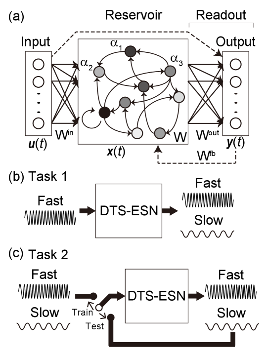
Methods.– The DTS-ESN consists of a reservoir with heterogeneous LI neurons and a linear readout as illustrated in Fig. 1(a). The DTS-ESN receives an input time series in the input layer, transforms it into a high-dimensional reservoir state , and produces an output time series as a linear combination of the states of the reservoir neurons. With distributed leak rates of reservoir neurons, the DTS-ESN extends greatly the range of timescales that can be realized by the LI-ESN [16].
In this study, the capability of the DTS-ESN is evaluated in two types of time series prediction tasks related to chaotic fast-slow dynamical systems. One is a one-step-ahead prediction task (Task 1) where input data are given only from the fast subsystem as depicted in Fig. 1(b). An inference of hidden slow dynamics from observational data of the fast dynamics is challenging but beneficial in reducing the effort involved in data measurement. An example in climate science is to predict slowly changing behavior in the deep ocean such as the temperature. The behavior is known to give an important feedback to the fast dynamical behavior of the atmosphere, land, and near-surface oceans [30], but the observation in the deep ocean remains as a major challenge [31]. The other is an autoregressive prediction task (Task 2) where a closed-loop version of the proposed model is used for a long-term prediction in a testing phase as illustrated in Fig. 1(c). RC approaches have shown a strong potential in long-term predictions of chaotic behavior [6, 7]. We examine the effect of distributed timescales of reservoir dynamics on the long-term prediction ability.
| Model | Equations | Fast | Slow | Parameter values |
| (i) Rulkov [32] | , , | |||
| (ii) Hindmarsh-Rose [33] | , | , , , | ||
| , | ||||
| (iii) tc-VdP [34] | , | , | , , | |
| , , | ||||
| (iv) tc-Lorenz [35] | , , | , , | , , | , , |
| , , | , , | |||
| , | , |
The DTS-ESN is formulated as follows:
| (1) | |||||
| (2) | |||||
| (5) |
where is the time, is the time step, is the reservoir state vector, is the identity matrix, is the diagonal matrix of leak rates for , is the internal state vector, is the element-wise activation function given as in this study, is the reservoir weight matrix with spectral radius , is the input weight matrix with input scaling factor , is the input vector, is the feedback weight matrix with feedback scaling factor , is the output vector, and is the output weight matrix. In the readout, we concatenate the reservoir state, the input, and the bias for Task 1 and use only the reservoir state for Task 2 as described in Eq. (5). Only is trainable and all the other parameters are fixed in advance [9, 13]. The DTS-ESN is reduced to the LI-ESN [16] if for all .
The fraction of non-zero elements in was fixed at , which were randomly drawn from a uniform distriubtion in [-1,1], and was rescaled so that its spectral radius equals 1. The entries of and were randomly drawn from a uniform distribution in . The leak rates were assumed to follow a reciprocal (or log-uniform) distribution in . This means that was randomly drawn from a uniform distribution in . The leak rate of neuron is represented as where denotes the time constant in the corresponding continuous-time model (see the Supplemental Material [36]).
In the training phase, an optimal output weight matrix is obtained by minimizing the following sum of squared output errors plus the regularization term:
| (6) |
where the summation is taken for all discrete time points in the training period, indicates the L2 norm, indicates the Frobenius norm, denotes the target dynamics, and represents the regularization factor [13]. In the testing phase, is used to produce predicted outputs.
| Model | ||||
|---|---|---|---|---|
| (i) Rulkov | 1 | 4000 | 8000 | 4000 |
| (ii) Hindmarsh-Rose | 0.05 | 200 | 1200 | 600 |
| (iii) tc-VdP | 0.01 | 50 | 150 | 100 |
| (iv) tc-Lorenz | 0.01 | 30 | 60 | 30 |
Analyses.– The timescales of the reservoir dynamics in the DTS-ESN are mainly determined by the hyperparameters including the time step , the spectral radius , and the leak rate matrix . The timescales of reservoir dynamics in the linearized system of Eq. (1), denoted by for , are linked to the set of eigenvalues of its Jacobian matrix as follows (see the Supplemental Material [36]):
| (7) |
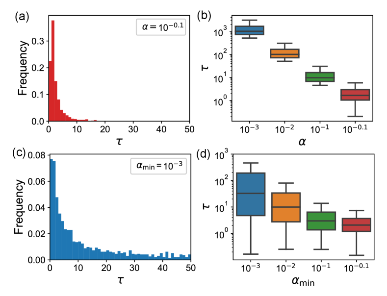
Figure 2 demonstrates that the timescale distribution in the linearized system is different between the LI-ESN and the DTS-ESN. Figure 2(a) shows a timescale distribution for the LI-ESN with . When is decreased to produce slower dynamics, the peak of the timescale distribution increases while the distribution range in the logarithmic scale is almost unaffected as shown in Fig. 2(b) [18]. Figure 2(c) shows a broader timescale distribution of the DTS-ESN with . As shown in Fig. 2(d), the distribution range monotonically increases with a decrease in (see the Supplemental Material [36]). The timescale analysis based on the linearized systems indicates that the DTS-ESN with a sufficiently small has much more diverse timescales than the LI-ESN.
Results.– We evaluated the computational performance of the DTS-ESN in prediction tasks involved with four chaotic fast-slow dynamical systems models listed in Table 1: (i) the Rulkov model which is a 2D map replicating chaotic bursts of neurons [32]; (ii) the Hindmarsh-Rose (HR) model which is a phenomenological neuron model exhibiting irregular spiking-bursting behavior [33]; (iii) the two coupled Van der Pol (tc-VdP) model which is a combination of fast and slow limit cycle oscillators with nonlinear damping [34]; (iv) the two coupled Lorenz (tc-Lorenz) model which is a caricature representing the interaction of the ocean with slow dynamics and the atmosphere with fast dynamics [35, 37]. There is a large timescale gap between the fast and slow subsystems.
We generated time series data from each dynamical system model using the parameter values listed in Table 1. The ODE models were numerically integrated using the Runge-Kutta method with time step . Then, we separated the whole time series data of total length into transient data of length , training data of length , and testing data of length . The transient data was discarded to wash out the influence of the initial condition of the reservoir state vector. We set the time step and the durations of data as listed in Table 2 unless otherwise noted.
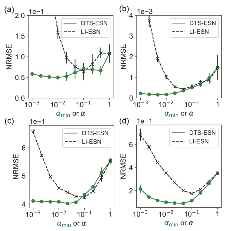
First, we performed the one-step-ahead prediction task (Task 1) using the open-loop model shown in Fig. 1(b), where the states of the whole variables at one step ahead are predicted only from the input time series of fast variables. The prediction performance is evaluated with the following Normalized Root Mean Squared Error (NRMSE) between the model predictions and the target outputs:
| NRMSE | (8) |
where denotes an average over the testing period.
Figures 3(a)-(d) show the comparisons between the DTS-ESN and the LI-ESN in the NRMSEs for the four dynamical systems models listed in Table 1 (see the Supplemental Material for examples of predicted time series [36]). The horizontal axis is for the DTS-ESN and for the LI-ESN. When , the two models coincide and yield the same performance. The prediction performance is improved as is decreased from 1 for the DTS-ESN, mainly due to an increase in the prediction accuracy with respect to the slow variables (see the Supplemental Material [36]). The DTS-ESN can keep a relatively small prediction error when is decreased even to in contrast to the LI-ESN. The best performance of the DTS-ESN is obviously better than that of the LI-ESN for all the target dynamical systems, indicating a higher ability of the DTS-ESN. Moreover, even with fixed at , the DTS-ESN can achieve the performance comparable to the best one obtained by the LI-ESN for all the target dynamics. This effortless setting of leak rates is an advantage of the DTS-ESN over the LI-ESN and the hierarchical LI-ESNs.
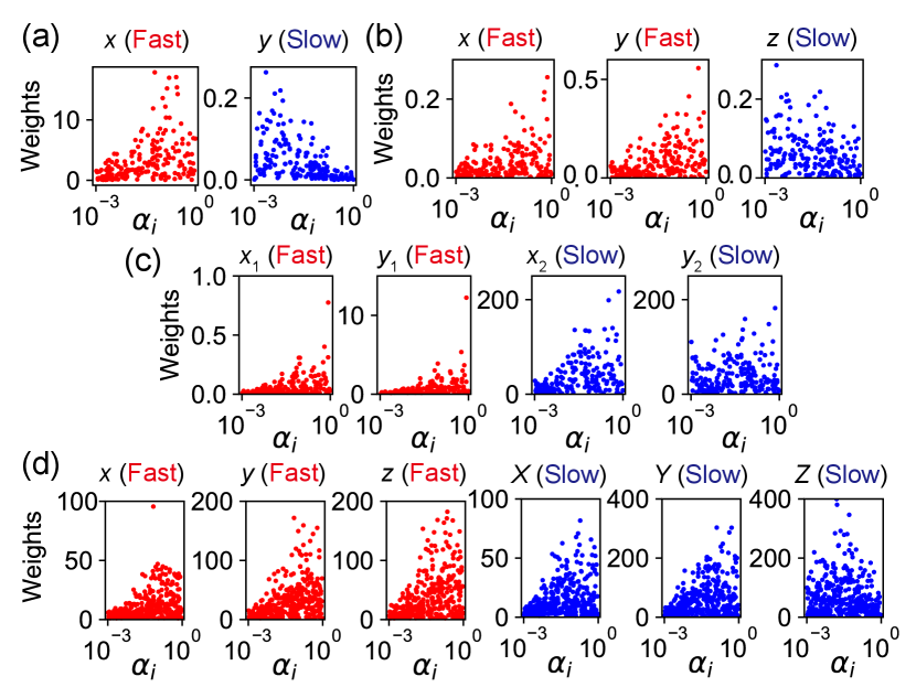
Figures 4(a)-(d) demonstrate the absolute output weights in of the trained DTS-ESNs, plotted against the leak rates of the corresponding neurons. Each panel corresponds to an output neuron for the variable specified by the label on that. The results indicate that the reservoir neurons with large , having small timescales, are mainly used for approximating the fast subsystems (red points) and those with small , having large timescales, are for the slow subsystems (blue points). We can see that the neuronal states with appropriate timescales are selected to comply with the timescale of the desired output as a result of model training. In Fig. 4(d) for the tc-Lorenz model, the reservoir neurons with relatively small are used for the slow variable but not for the other slow variables ( and ). This means that the dynamics of and are essentially not as slow as that of , causing the performance degradation with a large decrease in as shown in Fig. 3(d). By increasing the reservoir size and the length of training data, this degradation is mitigated (see Supplemental Material [36]). The natural separation of the roles of neurons can be regarded as a spontaneous emergence of modularization found in many biological systems [38, 39, 40].
Second, we performed the autoregressive prediction task (Task 2). As shown in Fig. 1(c), the open-loop model is trained using the training data, and then the closed-loop model is used to generate predicted time series autonomously. We increased from 60 in Table 2 to 120 for the tc-Lorenz model, in order to improve the prediction performance. In the testing phase, we evaluated the valid time [6] for the slow dynamics, indicating the elapsed time duration (measured in actual time units) before the normalized prediction error exceeds a threshold value in the testing phase. The error is defined as follows [7]:
| (9) |
where and represent the reservoir state vector and the target vector of slow variables, respectively, and denotes an average over the testing period.
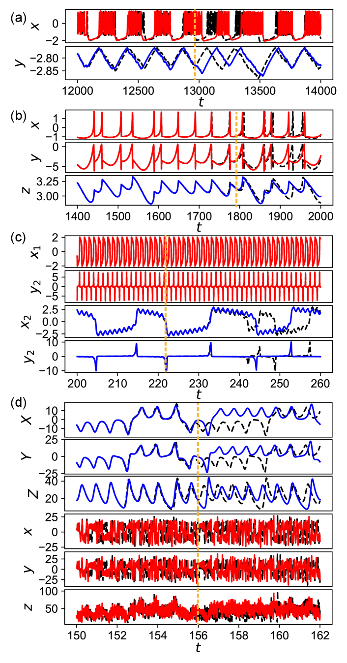
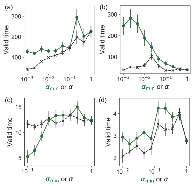
Figures 5(a)-(d) show examples of autoregressive predictions (red lines for fast variables and blue lines for slow ones) by the closed-loop DTS-ESN models for the four target dynamical systems. The predicted time series approximates well the target time series (black dashed lines) until the valid time indicated by the vertical dashed line. The divergence of the prediction error after a finite time is inevitable due to the chaotic dynamics. We note that, in Fig. 5(c) for the tc-VdP model, the discrepancy between the predicted and target time courses is not prominent until around but the normalized error exceeds at around . If the threshold value is changed to , the valid time is increased to around 44. Figures 6(a)-(d) demonstrate the comparisons of the valid time between the closed-loop DTS-ESN and the closed-loop LI-ESN for the four target dynamical systems. In all the panels, the largest valid time is achieved by the DTS-ESN, suggesting its higher potential in the long-term prediction. The valid time largely depends on the hyperparameter setting including the range of leak rates, which may be associated with the attractor replication ability of the DTS-ESN as measured by the Lyapunov exponents (see Supplemental Material [36] for details).
Discussion and conclusion.– We have proposed the RC model with diverse timescales, the DTS-ESN, by incorporating distributed leak rates into the reservoir neurons for modeling and prediction of multiscale dynamics. The results of the prediction tasks indicate the effectiveness of our randomization approach to realizing a reservoir with rich timescales. Although we assumed a specific distribution of leak rates in this study, another distribution could further improve the prediction performance. Moreover, another type of heterogeneity of reservoir components could boost the ability of RC systems in approximating a wide variety of dynamical systems. Future applications include a prediction of large-scale spatiotemporal chaotic systems [6, 41] from partial observations and an inference of slow dynamics from experimentally measured data involved in real-world multiscale systems [31, 42].
Acknowledgmnents.– We thank Daisuke Inoue for fruitful discussion and Huanfei Ma for valuable comments. This work was performed as a project of Intelligent Mobility Society Design, Social Cooperation Program (Next Generation Artificial Intelligence Research Center, the University of Tokyo with Toyota Central R&D Labs., Inc.), and supported in part by JSPS KAKENHI Grant Numbers 20K11882 (GT), JP20H05921 (KA), JST-Mirai Program Grant Number JPMJMI19B1 (GT), JST CREST Grant Number JPMJCR19K2 (GT), JST Moonshot R&D Grant Number JPMJMS2021 (KA), AMED under Grant Number JP21dm0307009 (KA), and International Research Center for Neurointelligence at The University of Tokyo Institutes for Advanced Study (UTIAS) (GT, KA).
References
- Vlachos [2005] D. G. Vlachos, Advances in Chemical Engineering 30, 1 (2005).
- Matouš et al. [2017] K. Matouš, M. G. Geers, V. G. Kouznetsova, and A. Gillman, Journal of Computational Physics 330, 192 (2017).
- Deisboeck et al. [2011] T. S. Deisboeck, Z. Wang, P. Macklin, and V. Cristini, Annual Review of Biomedical Engineering 13, 127 (2011).
- Walpole et al. [2013] J. Walpole, J. A. Papin, and S. M. Peirce, Annual Review of Biomedical Engineering 15, 137 (2013).
- Weinan [2011] E. Weinan, Principles of multiscale modeling (Cambridge University Press, 2011).
- Pathak et al. [2018a] J. Pathak, B. Hunt, M. Girvan, Z. Lu, and E. Ott, Physical Review Letters 120, 024102 (2018a).
- Pathak et al. [2018b] J. Pathak, A. Wikner, R. Fussell, S. Chandra, B. R. Hunt, M. Girvan, and E. Ott, Chaos: An Interdisciplinary Journal of Nonlinear Science 28, 041101 (2018b).
- Alber et al. [2019] M. Alber, A. B. Tepole, W. R. Cannon, S. De, S. Dura-Bernal, K. Garikipati, G. Karniadakis, W. W. Lytton, P. Perdikaris, L. Petzold, et al., npj Digital Medicine 2, 1 (2019).
- Jaeger [2001] H. Jaeger, Bonn, Germany: German National Research Center for Information Technology GMD Technical Report 148, 13 (2001).
- Jaeger and Haas [2004] H. Jaeger and H. Haas, Science 304, 78 (2004).
- Maass et al. [2002] W. Maass, T. Natschläger, and H. Markram, Neural Computation 14, 2531 (2002).
- Verstraeten et al. [2007] D. Verstraeten, B. Schrauwen, M. d’Haene, and D. Stroobandt, Neural Networks 20, 391 (2007).
- Lukoševičius and Jaeger [2009] M. Lukoševičius and H. Jaeger, Computer Science Review 3, 127 (2009).
- Werbos [1990] P. J. Werbos, Proceedings of the IEEE 78, 1550 (1990).
- Lukoševičius [2012] M. Lukoševičius, in Neural networks: Tricks of the trade (Springer, 2012) pp. 659–686.
- Jaeger et al. [2007] H. Jaeger, M. Lukoševičius, D. Popovici, and U. Siewert, Neural Networks 20, 335 (2007).
- Jaeger [2007] H. Jaeger, Discovering multiscale dynamical features with hierarchical echo state networks, Tech. Rep. (Jacobs University Bremen, 2007).
- Manneschi et al. [2021] L. Manneschi, M. O. Ellis, G. Gigante, A. C. Lin, P. Del Giudice, and E. Vasilaki, Frontiers in Applied Mathematics and Statistics 6, 76 (2021).
- Tanaka et al. [2019] G. Tanaka, T. Yamane, J. B. Héroux, R. Nakane, N. Kanazawa, S. Takeda, H. Numata, D. Nakano, and A. Hirose, Neural Networks 115, 100 (2019).
- Gallicchio et al. [2017] C. Gallicchio, A. Micheli, and L. Pedrelli, Neurocomputing 268, 87 (2017).
- Tamura and Tanaka [2021] H. Tamura and G. Tanaka, Neural Networks 143, 550 (2021).
- Li and Tanaka [2022] Z. Li and G. Tanaka, Neurocomputing 467, 115 (2022).
- Akiyama and Tanaka [2022] T. Akiyama and G. Tanaka, IEEE Access 10, 28535 (2022).
- Di Volo and Destexhe [2021] M. Di Volo and A. Destexhe, Scientific reports 11, 1 (2021).
- Tanaka et al. [2016] G. Tanaka, R. Nakane, T. Yamane, D. Nakano, S. Takeda, S. Nakagawa, and A. Hirose, in International Conference on Neural Information Processing (Springer, 2016) pp. 187–194.
- Appeltant et al. [2011] L. Appeltant, M. C. Soriano, G. Van der Sande, J. Danckaert, S. Massar, J. Dambre, B. Schrauwen, C. R. Mirasso, and I. Fischer, Nature communications 2, 1 (2011).
- Paquot et al. [2012] Y. Paquot, F. Duport, A. Smerieri, J. Dambre, B. Schrauwen, M. Haelterman, and S. Massar, Scientific reports 2, 1 (2012).
- Stelzer et al. [2020] F. Stelzer, A. Röhm, K. Lüdge, and S. Yanchuk, Neural Networks 124, 158 (2020).
- Pauwels et al. [2019] J. Pauwels, G. Verschaffelt, S. Massar, and G. Van der Sande, Frontiers in Physics , 138 (2019).
- Seshadri [2017] A. K. Seshadri, Climate Dynamics 48, 2235 (2017).
- Meinen et al. [2020] C. S. Meinen, R. C. Perez, S. Dong, A. R. Piola, and E. Campos, Geophysical Research Letters 47, e2020GL089093 (2020).
- Rulkov [2001] N. F. Rulkov, Physical Review Letters 86, 183 (2001).
- Hindmarsh and Rose [1984] J. L. Hindmarsh and R. Rose, Proceedings of the Royal Society of London. Series B. Biological Sciences 221, 87 (1984).
- Champion et al. [2019] K. P. Champion, S. L. Brunton, and J. N. Kutz, SIAM Journal on Applied Dynamical Systems 18, 312 (2019).
- Boffetta et al. [1998] G. Boffetta, P. Giuliani, G. Paladin, and A. Vulpiani, Journal of the Atmospheric Sciences 55, 3409 (1998).
- [36] See supplementary material at [http://link.aps.org/supplemental/10.1103/PhysRevResearch.4.L032014] for further details.
- Borra et al. [2020] F. Borra, A. Vulpiani, and M. Cencini, Physical Review E 102, 052203 (2020).
- Kashtan and Alon [2005] N. Kashtan and U. Alon, Proceedings of the National Academy of Sciences 102, 13773 (2005).
- Lorenz et al. [2011] D. M. Lorenz, A. Jeng, and M. W. Deem, Physics of life reviews 8, 129 (2011).
- Yang et al. [2019] G. R. Yang, M. R. Joglekar, H. F. Song, W. T. Newsome, and X.-J. Wang, Nature neuroscience 22, 297 (2019).
- Vlachas et al. [2020] P. R. Vlachas, J. Pathak, B. R. Hunt, T. P. Sapsis, M. Girvan, E. Ott, and P. Koumoutsakos, Neural Networks 126, 191 (2020).
- Proix et al. [2018] T. Proix, V. K. Jirsa, F. Bartolomei, M. Guye, and W. Truccolo, Nature Communications 9, 1 (2018).