Resistive Anomaly near a Ferromagnetic Phase Transition:
A Classical Memory Effect

Second-order phase transitions are accompanied by diverging order-parameter fluctuations near the critical temperature $T_{c}$. A classic manifestation is critical opalescence— strong scattering of light by a fluid near its critical point. In metals approaching a magnetic or structural transition, electron waves are similarly scattered by critical fluctuations. The metallic analog of critical opalescence is a knee- or cusp-like anomaly in the temperature dependence of resistivity near $T_{c}$.

Since the pioneering work of Gerlach [2], resistive anomalies have been widely observed in elemental metallic ferromagnets (FMs), such as Ni, Fe, Co, and Gd [3], in rare-earth intermetallics [4, 5], and in metallic antiferromagnets (AFMs), including elemental (Tb, Ho) [6], intermetallic [7], and iron pnictides [8]. Similar anomalies also occur near structural transitions, e.g., near order-disorder transitions in binary alloys [9] and the cubic-to-tetragonal transition in doped SrTiO₃ [10].

Resistive anomalies offer two main advantages: they enable rapid identification of magnetic transitions without direct magnetic measurements, and their shapes reveals information about critical exponents. This is particularly valuable given the higher precision of resistivity measurements compared to specific heat. However, extracting such information requires a suitable theoretical framework [11], which we revisit and refine in this Letter.

Theoretical studies of resistive anomalies began with de Gennes and Friedel (dGF) [12], who attributed the resistive anomaly near a FM transition to spin-flip scattering of free electrons by localized magnetic moments. Modeling this as quenched long-range disorder (LRD), they computed the transport scattering time $\tau_{\rm tr}$, using the Fermi’s Golden Rule (FGR):

$\displaystyle 1/\tau_{\rm tr}\propto\int_{q\leq 2k_{F}}d^{d}q\,\frac{q^{2}}{2k_{\mathrm{F}}^{2}}\,\Delta t(q)\,W({\bf q}),$

(1)

where $k_{\mathrm{F}}$ is the Fermi momentum, $W({\bf q})=\langle\delta{\bf S}_{{\bf q}}\cdot\delta{\bf S}_{-{\bf q}}\rangle$ is the connected spin correlation function, $\Delta t(q)=1/\varv_{\mathrm{F}}q$ arises from the energy-conserving delta-function averaged over directions of ${\bf q}$, and the “transport factor”–$q^{2}/2k_{\mathrm{F}}^{2}$–suppresses small-angle scattering. In the mean-field theory, $W(q)\propto\left(({\bf q}-{\bf Q})^{2}+\xi^{-2}\right)^{-1}$, where the correlation length $\xi\propto|\theta|^{-1/2}$ and $\theta=(T-T_{c})/T_{c}$. For FMs, ${\bf Q}=0$ and thus Eq. (1) is dominated by $q\sim k_{\mathrm{F}}$. Subtracting off this non-universal part, dGF retained only the critical contribution from $q\sim\xi^{-1}\ll k_{\mathrm{F}}$, leading to a resistivity cusp: $\delta\rho_{\rm dGF}\propto-|\theta|\ln(1/|\theta|)$ in $d=3$ and $\delta\rho_{\rm dGF}\propto-|\theta|^{1/2}$ in $d=2$.

Ten years later, Fisher and Langer (FL) [1] challenged two key aspects of dGF’s analysis. First, they correctly pointed out that impurity and phonon scattering—which plays the role pf short-range disorder (SRD)—cannot be treated independently of magnetic scattering, if the corresponding mean free path $\ell_{\mathrm{s}}$ is shorter than $\xi$; a condition inevitably met near $T_{c}$. While FL conjectured that this interplay would weaken the dGF singularity, they did not provide a quantitative treatment. Instead, they focused on the second issue: the short-range ($q\sim k_{\mathrm{F}}$) contribution to Eq. (1), discarded by dGF, but which, in fact, contributes to the critical $\theta$-dependence. Noting that in typical metallic magnets $k_{\mathrm{F}}\sim a^{-1}_{\rm M}\sim a^{-1}$, where $a_{\rm M}$ is the spacing between magnetic moments and $a$ the lattice constant, FL observed that the upper limit of the integral in Eq. (1) probes the short-distance part of the spin correlation function. This contribution to $1/\tau_{\rm tr}$ scales with temperature as the magnetic internal energy, $U(T)$. Beyond the mean-field theory, the specific heat $C(T)=dU/dT\propto|\theta|^{-\alpha}$, with $0<\alpha<1$, leading FL to conclude that $d\delta\rho/dT\propto d\tau_{\rm tr}^{-1}/dT\propto C(T)$, or

$\displaystyle\delta\rho_{\rm FL}\propto\text{sgn}\,\theta\,|\theta|^{1-\alpha},$

(2)

which is known as “FL scaling”. Unlike the dGF prediction, FL scaling implies that $\rho(T)$ is a monotonic—generally increasing—function of $\theta$ [13], with a cusp in its derivative at $T_{c}$, consistent with observations in elemental FMs away from the critical point [3].

While FL’s argument applies to both FMs and AFMs, Suezaki and Mori (SM) [14] pointed out an additional short-range contribution in metallic AFMs with $Q\sim k_{\mathrm{F}}\sim a^{-1}$. In this case, the region ${\bf q}\approx{\bf Q}$ contributes critically to the integral (1), while neither the transport factor nor $\Delta t(q)$ affect the scaling. On changing variables to ${\bf q}^{\prime}={\bf q}-{\bf Q}$, the integral is dominated by $q^{\prime}\sim\xi^{-1}$, yielding

$\displaystyle\delta\rho_{\rm SM}\propto\int dq^{\prime}\,q^{\prime d-1}W(q^{\prime})=\langle\delta M^{2}\rangle\propto|\theta|^{2\beta},$

(3)

where $\delta M$ is the fluctuation of the magnetic order parameter and $\beta$ is the critical exponent, defined by $\langle M\rangle\propto(-\theta)^{\beta}$ for $\theta<0$.

Here, we show that in the diffusive regime ($\xi\gg\ell_{\mathrm{s}}$), Eq. (3) applies not only to AFMs but also to FMs. In this case, the anomaly originates from long-range critical fluctuations—the same mechanism considered by dGF. Our result departs from dGF’s prediction due to the breakdown of Matthiessen’s rule, as noted by FL. Crucially, when properly accounted for, this breakdown enhances rather than suppresses the resistive anomaly. While Ref. [15] attributed such enhancement to mesoscopic fluctuations, we demonstrate that even classical diffusive motion of phase-incoherent electrons in a background of long-range magnetic fluctuations produces a competing mechanism to FL scaling. The effect stems from a classical memory mechanism: repeated returns of a diffusive trajectory to the same location.

As in previous work, we treat spin-flip scattering as arising from quenched long-range disorder (LRD), characterized by the correlation function $W(q)=\int d^{d}r\,e^{i{\bf q}\cdot{\bf r}}\langle V({\bf r})V(0)\rangle$. This approximation is justified in the small-$q$ limit, where critical fluctuations exhibit critical slowing down: their relaxation time diverges as $q^{-z}$ near a continuous phase transition, with $z$ the dynamical exponent [16]. Assuming that LRD is weaker than SRD, the key question is: what is the resulting resistivity of the metal?

Classical electrodynamics offers a partial answer to this question [17]. In the diffusive regime, regions of size $\sim\xi$ act as local Ohmic resistors with spatially varying conductivity $\sigma({\bf r})$. Consequently, both the electric field and current density fluctuate, while obeying Ohm’s law: ${\bf j}({\bf r})=\sigma({\bf r}){\bf E}({\bf r})$. The measured conductivity is defined via the relation between averaged quantities $\langle{\bf j}\rangle=\sigma_{\rm exp}\langle{\bf E}\rangle$, where $\langle{\bf E}\rangle$ is is the ratio of the voltage to sample length [18]. For weak fluctuations, $\sigma_{\rm exp}$ splits into two contributions [19]:

$\displaystyle\sigma_{\rm exp}=\sigma_{\rm K}+\delta\sigma_{\rm fl},$

(4)

where $\sigma_{\rm K}$ is the Kubo conductivity in a uniform field, and $\delta\sigma_{\rm fl}$ is a correction due to spatial inhomogeneity. The result of Ref. [17] for a weakly inhomogeneous medium translates into $\delta\sigma_{\rm fl}=-\langle\delta\sigma^{2}\rangle/d\,\sigma_{\rm K}$ [18, 19, 15]. In our context, these conductivity fluctuations stem from order-parameter fluctuations, implying $\delta\sigma_{\rm fl}\propto\langle\delta M^{2}\rangle$, thus justifying the scaling in Eq. (3).

The Kubo conductivity itself consists of two parts: $\sigma_{\rm K}=\sigma_{\rm s}+\delta\sigma_{\ell}$, where $\sigma_{\rm s}$ is the Drude contribution from SRD and $\delta\sigma_{\ell}$ is the correction due to LRD. The form of $\delta\sigma_{\ell}$ depends on the relation between $\xi$ and $\ell_{\mathrm{s}}$, with the key quantity being the “interaction time” $\Delta t(q)$ in Eq. (1), which is the duration of a scattering event with momentum transfer $q\sim\xi^{-1}$ [20]. By the uncertainty principle, such momentum transfer occurs within a region of size $\sim 1/q$.

In the ballistic regime ($\xi\ll\ell_{\mathrm{s}}$), an electron traverses this region in time $\Delta t(q)\sim\xi/\varv_{\mathrm{F}}\ll\tau_{\mathrm{s}}=\ell_{\mathrm{s}}/\varv_{\mathrm{F}}$, so SRD and LRD act independently, and their scattering rates add according to Matthiessen’s rule.

In the diffusive regime ($\xi\gg\ell_{\mathrm{s}}$), scattering by SRD broadens electron states, requiring the energy-conserving delta function in FGR to be replaced by a Lorentzian of width $1/\tau_{\mathrm{s}}$ [21, 22, 23, 24]. Consequently, $\Delta t(q)\sim\tau_{\mathrm{s}}=\text{const}$, and the integrand in Eq. (1) becomes less singular as $q\to 0$, thus weakening the dGF anomaly. However, the dominant effect of diffusion is that it significantly enhances the time required for an electron to traverse a region of size $\sim\xi$, now given by $\Delta t(q)\sim 1/D_{\rm s}q^{2}$, where $D_{\rm s}=\varv_{\mathrm{F}}^{2}\tau_{\mathrm{s}}/d$ is the diffusion coefficient due to SRD. As a result, the integrand in Eq. (1) becomes more singular than in the ballistic regime: the $1/q^{2}$ divergence in $\Delta t(q)$ cancels the $q^{2}$ transport factor, reducing the integral to $\int dq\,q^{d-1}W(q)\sim\langle\delta M^{2}\rangle$. Thus, $\delta\sigma_{\ell}\sim\delta\sigma_{\rm fl}\propto\langle\delta M^{2}\rangle$, consistent with Eq. (3).

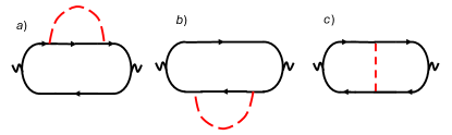
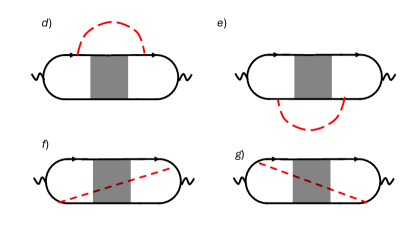
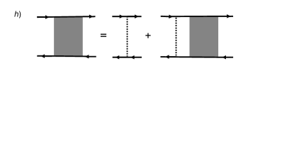
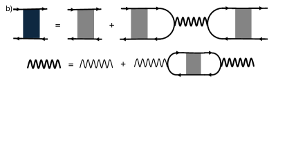
We now outline the main steps of the derivation. We consider a metal with parabolic dispersion $\varepsilon_{\bf k}=k^{2}/2m-\mu$, subject to the condition $\mu\tau_{\mathrm{s}}\gg 1$, where $\mu$ is the chemical potential. The leading corrections to the Kubo term in Eq. (4) due to LRD are captured by diagrams a–g in Fig. 1. Solid lines represent disorder-averaged retarded/advanced Green’s functions,

$\displaystyle G^{R/A}_{\bf k}(\omega)=\frac{1}{\omega-\varepsilon_{\bf k}\pm i\tau_{\mathrm{s}}/2},$

(5)

while dashed and dotted lines correspond to the correlation functions of LRD and SRD, respectively. The shaded box denotes the diffuson ladder $\mathcal{L}^{R}(q,\omega)$, which satisfies the integral equation shown in panel h. Diagrams a–c were previously analyzed in Ref. [25], but only for $Q\ell_{\mathrm{s}}\gg 1$, which excludes the FM case. Diagrams d–g were shown in Ref. [26] to reflect a classical memory effect in the optical conductivity: a power-law, rather than exponential, decay of the velocity-velocity correlation function at long times [27, *Hauge:1974].

In general, the correlator of magnetic fluctuations in a FM can be written as

$\displaystyle W(q)=q^{-2+\eta}F(q\xi),$

(6)

where $F(x)$ is a universal scaling function. Using the $\epsilon$-expansion and renormalization group, its asymptotic form for $q\xi\gg 1$ was found to be [29, 30]:

$\displaystyle F(q\xi\gg 1)=A+B_{\pm}\,\text{sgn}\,\theta\left(\frac{|\theta|}{q^{1/\nu}}\right)^{1-\alpha}+C_{\pm}\frac{|\theta|}{q^{1/\nu}}+\dots,$

(7)

with $A>0$, and $B_{\pm}$, $C_{\pm}$ generally different above and below $T_{c}$. The critical exponents $\alpha$, $\eta$, and $\nu$ for common universality classes are listed in Table 1.

The sum of diagrams a–c in Fig. 1 gives the following correction to the dc conductivity

$\displaystyle\delta\sigma_{\ell,a\text{--}c}=-\frac{e^{2}}{2\pi dm^{2}}\int_{\bf q}q^{2}W(q)\int_{\bf k}\left|G_{{\bf k}-{\bf q}/2}^{R}(0)G_{{\bf k}+{\bf q}/2}^{R}(0)\right|^{2},$

(8)

where $\int_{\bf p}\equiv\int d^{d}p/(2\pi)^{d}$. The overall $q^{2}$ factor is the same transport factor as in Eq. (1). The momentum integral is evaluated using $\int_{\bf k}=\nu_{\text{F}}\int d\varepsilon_{\bf k}\int_{\hat{k}}$, with $\nu_{\text{F}}$ the density of states at the Fermi level and $\int_{\hat{k}}$ denoting angular averaging. For $q\sim\xi^{-1}\ll k_{\mathrm{F}}$, the dispersion simplifies to $\varepsilon_{{\bf k}\pm{\bf q}/2}\approx\varepsilon_{\bf k}\pm\varv_{\mathrm{F}}\hat{k}\cdot{\bf q}/2$, yielding

$\displaystyle\delta\rho_{\ell,a\text{--}c}/\rho_{\mathrm{s}}=-\delta\sigma_{\ell,a\text{--}c}/\sigma_{\rm s}=(\tau_{\mathrm{s}}^{2}/k_{\mathrm{F}}^{2})\int_{\bf q}q^{2}W(q)f_{d}(q\ell_{\mathrm{s}}),$

(9)

with $\rho_{\mathrm{s}}=1/\sigma_{\rm s}$, $f_{2}(x)=1/\sqrt{x^{2}+1}$, and $f_{3}(x)=\tan^{-1}x/x$. For $q\gg\ell_{\mathrm{s}}^{-1}$, Eq. (9) is reduced back to FGR, Eq. (1). The FL result [Eq. (2)] arises from the second term in Eq. (7), and is present in both ballistic and diffusive regimes. Subtracting it off, the remaining contribution from $q\sim\xi^{-1}$ scales as $\delta\rho_{a\text{--}c}\propto|\theta|^{(d-1+\eta)\nu}$, which generalizes the dGF result beyond the mean-field level. In this limit, Matthiessen’s rule holds: $\delta\rho_{a\text{--}c}=\rho_{\mathrm{s}}(\tau_{\mathrm{s}}/\tau_{\rm tr})$. In the diffusive regime ($q\ll\ell_{\mathrm{s}}^{-1}$), $f_{d}(x)\approx f_{d}(0)=1$, which adds an extra $q$ factor to the integrand and yields $\delta\rho_{a\text{--}c}\propto|\theta|^{(d+\eta)\nu}$, thus confirming that the dGF anomaly is weakened compared to the ballistic case.

Diagrams d–g in Fig. 1, which are of primary interest here, yield

$\displaystyle\delta\sigma_{\ell,d-g}=-\frac{4e^{2}}{\pi d}\int_{\bf q}W(q)\mathcal{L}^{R}(q,0)\left({\mathrm{Im}}\,{\bf u}_{\bf q}\right)^{2},$

(10)

where ${\bf u}_{\bf q}=\int_{\bf k}({\bf k}/m)\left|G^{R}_{\bf k}(0)\right|^{2}G^{A}_{{\bf k}+{\bf q}}(0)$ is the current vertex and $\mathcal{L}^{R}(q,0)$ is the static diffuson ladder, given by $\mathcal{L}^{R}(q,0)=(1/2\pi\nu_{\text{F}}\tau_{\mathrm{s}})\mathcal{D}_{d}(q\ell_{\mathrm{s}})$ with $\mathcal{D}_{2}(x)=\left(1-1/\sqrt{x^{2}+1}\right)^{-1}$ and $\mathcal{D}_{3}(x)=\left(1-\tan^{-1}x/x\right)^{-1}$. The limit $\mathcal{L}^{R}(q\to 0,0)\propto 1/q^{2}$ corresponds to the diffusive limit of the interaction time, $\Delta t(q)$ in Eq. (1). Integrating over ${\bf k}$, we obtain

$\displaystyle\frac{\delta\rho_{\ell,d-g}}{\rho_{\mathrm{s}}}=-\frac{\delta\sigma_{\ell,d-g}}{\sigma_{\rm s}}=\frac{1}{4\mu^{2}}\int_{\bf q}W(q)\mathcal{D}_{d}(q\ell_{\mathrm{s}})g_{d}(q\ell_{\mathrm{s}}).$

(11)

where $g_{2}(x)=x^{2}/(1+x^{2})^{3}$ and $g_{3}(x)=x^{2}/(1+x^{2})^{2}$. In the ballistic limit, $\delta\rho_{\ell,d-g}\ll\delta\rho_{\ell,a-c}$. In the diffusive limit, one can replace $\mathcal{D}_{d}(x)$ and $g_{d}(x)$ in Eq. (11) by their small-$x$ limits, i.e., by $d/x^{2}$ and $x^{2}$, respectively, which yields

$\displaystyle\delta\rho_{\ell,d-g}/\rho_{\mathrm{s}}=(d/4\mu^{2})\int_{\bf q}W(q)=(d/4)\langle V^{2}\rangle/\mu^{2},$

(12)

where $\langle V^{2}\rangle=\int_{\bf q}W(q)$ is the variance of the potential energy due to LRD. $\delta\rho_{\ell,d-g}$ is obviously more singular than $\delta\rho_{\ell,a-c}$ in the diffusive limit, and thus the latter can be neglected.

Finally, we come to the second, fluctuational term in Eq. (4), which becomes relevant in the diffusion limit, when a region of size $\sim\xi$ can be assigned its own conductivity. At fixed $\mu$, fluctuations of the local conductivity result from fluctuations of the Fermi energy. If $\sigma_{\rm s}\left[\varepsilon_{\text{F}}({\bf r})\right]=\sigma_{\rm s}\left[\mu-V({\bf r})\right]$ is the local conductivity due to SRD at fixed Fermi energy, then $\langle\delta\sigma_{\rm fl}^{2}\rangle=\langle\sigma_{\rm s}^{2}\left[\mu-V({\bf r})\right]\rangle-\langle\sigma_{\rm s}\left[\mu-V({\bf r})\right]\rangle^{2}\approx\langle V^{2}\rangle\left(\partial\sigma_{\rm s}(\mu)/\partial\mu\right)^{2}=\left(\langle V^{2}\rangle/\mu^{2}\right)\sigma_{\rm s}^{2}$, where at the last step we took into account that $\nu(\epsilon)\tau_{\mathrm{s}}(\epsilon)={\rm const}$ for SRD. Therefore, the fluctuational correction equals to $\delta\rho_{\rm fl}/\rho_{\rm s}=-\delta\sigma_{\rm fl}/\sigma_{\rm s}=\langle V^{2}\rangle/d\,\mu^{2}$, which is of the same order as the Kubo contribution in Eq. (12). Adding up the Kubo and fluctuational corrections gives the final result in the diffusive limit:

$\displaystyle\delta\rho/\rho_{\rm s}=(d/4+1/d)\langle V^{2}\rangle/\mu^{2}.$

(13)

Substituting Eq. (7) into Eq. (13), integrating term by term over the interval $1/\xi\lesssim q\lesssim 1/\ell_{\mathrm{s}}$, and keeping only the contribution from the lower limit ¹¹1Here, we assume the most common scenario in which the integral of $W(q)$ up to the upper cutoff $1/l_{s}$ remains far from saturating the sum rule $\int_{\rm BZ}W(q)\,d^{d}q=NS^{2}$, where $N$ is the total number of spins., we arrive at the scaling form in Eq. (3):

$\displaystyle\delta\rho\propto A^{\prime}|\theta|^{2\beta}=A^{\prime}|\theta|^{1-\alpha-\zeta},$

(14)

where $2\beta=(d-2+\eta)\nu>0$, $\zeta=(2-\eta)\nu-1$, and where the hyperscaling relation $\nu d=2-\alpha$ [32] was employed at the last step. The dominant singular contribution in the diffusive regime scales like the Bragg peak intensity (square of the order parameter). As long as $\zeta>0$, the “diffusive anomaly” in Eq. (14) is more singular than the FL one, Eq. (2). Table 1 confirms that this holds for the most common universality classes. The sign of the diffusive anomaly–whether it manifests as a cusp or anti-cusp in $\rho$–is non-universal, as it depends on the relative magnitudes of the constants $A$, $B_{\pm}$, and $C_{\pm}$ in Eq. (7). In particular, $\delta\rho$ in Eq. (14) exhibits a cusp at $\theta=0$ if $A^{\prime}<0$ and an anti-cusp if $A^{\prime}>0$.

We now turn to the anomaly in the optical conductivity. Following Ref. [26], we initially ignore the effect of electron-electron interaction on diffusion, and also focus on the regime of $\Omega\tau_{\mathrm{s}}\ll 1$, when the frequency enters only through the diffuson as ${\mathcal{L}}^{R}(q,\Omega)=(1/2\pi\nu_{F}\tau_{\mathrm{s}}^{2})(D_{\mathrm{s}}q^{2}-i\Omega)^{-1}$, while the rest of a diagram can be evaluated at zero frequency. In this regime, the dominant contribution to the optical conductivity is given by diagrams d-g. At finite $\Omega$, Eq. (10) is replaced by

$\displaystyle{\mathrm{Re}}\delta\sigma(\Omega)=-\frac{4e^{2}}{\pi d}\int_{\bf q}W(q){\mathrm{Re}}\mathcal{L}^{R}(q,\Omega)\left({\mathrm{Im}}\,{\bf u}_{\bf q}\right)^{2}.$

(15)

In the diffusive limit, $({\mathrm{Im}}\,{\bf u}_{\bf q})^{2}=(\pi\nu_{\text{F}}\tau_{\mathrm{s}}/k_{\mathrm{F}})^{2}(q\ell_{\mathrm{s}})^{2}$, which yields for $\Delta{\mathrm{Re}}\sigma(\Omega)\equiv{\mathrm{Re}}\delta\sigma(\Omega)-\delta\sigma(0)$:

$\displaystyle\Delta{\mathrm{Re}}\sigma(\Omega)=\frac{d}{2}\sigma_{\mathrm{s}}\frac{\Omega^{2}}{E_{F}^{2}}\int_{\bf q}\frac{W(q)}{(D_{\mathrm{s}}q^{2})^{2}+\Omega^{2}},$

(16)

where $\sigma_{\mathrm{s}}=1/\rho_{\mathrm{s}}$. For $\Omega\ll D_{\mathrm{s}}/\xi^{2}$, one can set $q=0$ in $W(q)$ and factor it out from the integral, yielding

$\displaystyle\Delta{\mathrm{Re}}\sigma(\Omega)=b_{d}\sigma_{\mathrm{s}}\left(\frac{|\Omega|}{D_{\mathrm{s}}}\right)^{d/2}\frac{W(0)}{\mu^{2}},$

(17)

where $b_{2}=1/16$ and $b_{3}=\sqrt{2}/16\pi$. For $D_{\mathrm{s}}/\xi^{2}\ll\Omega\ll 1/\tau_{\mathrm{s}}$, one can neglect the $(D_{\mathrm{s}}q^{2})^{2}$ term in the denominator, arriving at the $\Omega$-independent value: $\Delta{\mathrm{Re}}\sigma(\Omega)=-\sigma_{\mathrm{s}}(d/4)\langle V^{2}\rangle/\mu^{2}$. Finally, the conventional Drude behavior is recovered for $\Omega\gg 1/\tau_{s}$, i.e., ${\mathrm{Re}}\sigma(\Omega)\propto 1/\Omega^{2}\tau_{\mathrm{s}}$. Note that a nonanalytic frequency dependence comes only from the Kubo part of the measured conductivity, whereas the fluctuational part gives the usual Drude behavior.

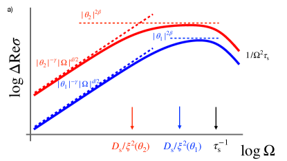
The behavior of the optical conductivity near a phase transition is sketched in Fig. 2 for two reduced temperatures, $|\theta|_{1}>|\theta|_{2}$. The slope of the nonanalytic part at lower frequencies is proportional to $W(0)\propto|\theta|^{-\gamma}$. The non-analytic range is bounded from above by the Thouless energy at length $\xi$, $E_{\rm Th}(|\theta|)=D_{\mathrm{s}}/\xi^{2}(|\theta|)\propto|\theta|^{2\nu}$, which vanishes for $T\to T_{c}$. In the intermediate range, above $E_{\rm Th}(|\theta|)$ but below $1/\tau_{\mathrm{s}}$, the optical conductivity reaches a plateau at a value that scales with $|\theta|$ is the same was as the dc resistivity, i.e., as $|\theta|^{2\beta}$. (We assume here that $\delta\rho$ in Eq. (14) has a cusp at $\theta=0$).

As shown in Ref. [33], however, Coulomb interaction modifies electron diffusion. In the presence of dynamic screening, the bare diffuson (shaded box in Fig. 2b) is replaced by the screened one, $\mathcal{L}^{R}_{\rm sc}(q,\omega)$ (black box), as depicted in the first line of panel b), where the thick wavy line represents the dynamically screened interaction $U^{R}_{\rm sc}(q,\omega)$. This is related to the bare interaction $U_{0}(q)$ via the random-phase approximation (second line). For $q\ell_{\mathrm{s}}\ll 1$ and $\omega\tau_{\mathrm{s}}\ll 1$, the screened diffuson reads

$\displaystyle\mathcal{L}^{R}_{\rm sc}(q,\Omega)$

$\displaystyle=$

$\displaystyle\frac{1}{2\pi\nu_{\text{F}}\tau_{\mathrm{s}}^{2}}\frac{1+\nu_{\text{F}}U_{0}(q)}{D_{\mathrm{s}}q^{2}\left(1+\nu_{\text{F}}U_{0}(q)\right)-i\Omega}.$

(18)

At $\Omega=0$, this reduces to the singular static form $\propto 1/q^{2}$, implying no change to the dc conductivity. For finite $\Omega$, and with bare Coulomb interaction $U_{0}(q)\propto 1/q^{d-1}$, the denominator becomes $D_{\mathrm{s}}q^{3-d}\kappa_{d}^{d-1}-i\Omega$, which eliminates the diffusion pole and suppresses the non-analyticity in $\sigma(\Omega)$.²²2In $d=2$, a weak nonanalyticity survives: $\Delta{\mathrm{Re}}\sigma(\Omega)\propto\Omega^{2}\ln\Omega^{-1}$ for $\Omega\ll D_{\mathrm{s}}\kappa_{2}/\xi$. Here, $\kappa_{d}$ denotes the inverse screening length in $d$ dimensions.

Nevertheless, we propose two scenarios in which non-analytic behavior in $\sigma(\omega)$ may still be observable. The first, originally proposed in Ref. [33], involves a $d=2$ electron system screened by a metallic gate. The gate transforms the bare Coulomb potential into a dipolar one, yielding $U_{0}(q\to 0)=\text{const}$, so screening leads only to an irrelevant renormalization of the diffusion coefficient. We therefore suggest measuring $\sigma(\Omega)$ near a ferromagnetic transition in a gated 2D metal, such as Fe_3-xGeTe₂.

The second scenario involves a ferroelectric transition in a weakly doped insulator, where the divergence of the lattice dielectric constant, $\epsilon_{\rm L}$, near $T_{c}$ suppresses Coulomb interaction among itinerant electrons. For this mechanism to be effective, the inverse screening length must vanish faster than the correlation length. In $d=3$, $\kappa_{3}\propto|\theta|^{\gamma/2}$ and $\xi\kappa_{3}\propto|\theta|^{\gamma/2-\nu}$, which only vanishes if $\gamma>2\nu$—a condition marginally satisfied for 3D Ising transitions [35]. In $d=2$, however, $\kappa_{2}\propto|\theta|^{\gamma}$, so $\xi\kappa_{2}\to 0$ requires only $\gamma>\nu$, which holds for the 2D Ising class. We thus propose probing the optical conductivity near the phase transition in weakly doped 2D ferroelectrics such as $\alpha$-In₂Se₃, which undergoes a second-order transition in both bulk [36] and exfoliated forms [37], and can be doped [38], or in monolayer SnTe [39]. At low doping, carriers near $T_{c}$ are likely to be non-degenerate, but this does not affect the resistive anomaly, which remains a single-particle effect. Our results extend to this regime by replacing $\varepsilon_{\text{F}}\to T$.

While resistive anomalies near $T_{c}$ are widely observed in metallic ferromagnets [2, 44, 45, 3], the scaling predicted by Fisher and Langer (FL) is not universally obeyed. In some cases, such as Ni, the anomaly aligns with FL scaling over a finite temperature range [11], whereas in others, like the rare-earth FMs RNi₅ (R = Tb, Dy, Er), $\rho$ itself—not $d\rho/dT$—peaks at $T_{c}$, deviating from FL behavior [5]. Even for Ni, fitting the data using only FL singular and regular terms fails within $\pm 1$ K of $T_{c}$ [11].

In contrast to the FL anomaly, which produces a peak in $d\rho/dT$, the diffusive mechanism discussed in this Letter yields a cusp or anticusp in $\rho$, consistent with the resistivity peak observed in RNi₅ [5]. A similar cusp in $\rho$, together with an asymmetric peak-antipeak structure in $d\rho/dT$ from the sum of regular and singular contributions, may also explain the anomaly seen in GaR₂ FMs (R = Ni, Rh, Pt) [4].

Resolving the FL and diffusive contributions may require measurements too close to $T_{c}$ for conclusive interpretation. A more robust signature is the non-Drude behavior of the optical conductivity, shown in Fig. 2, which reflects classical memory effects. However, such behavior is only expected in gated $d=2$ systems or near ferroelectric transitions.

An alternative route is to study periodic intermetallic magnets, where the spacing between localized moments matches $\ell_{\mathrm{s}}$, thus extending the temperature range of the diffusive regime near $T_{c}$. These systems may permit extraction of the $\beta$ exponent from transport and its comparison to neutron scattering data. Ongoing efforts also aim to realize 2D analogs of such materials [46].

Note added in proof: Recent non-linear optical experiments on ferromagnetic Ca₂RuO₄ (Bhandia et al., arXiv:2412.08749) confirmed that scattering by magnetic moments is elastic and revealed a cusp in the momentum relaxation rate, consistent with our prediction.

We thank P. Armitage, G. Blumberg, A. Chubukov, V. Kravtsov, S. Kundu, A. Levchenko, S. Kivelson, A. McLeod, A. Mirlin, B. Shklovskii, Y. Wang, and K. Alp Yay for illuminating discussions. We are especially grateful to D. Polyakov for bringing Ref. [33] to our attention. DLM acknowledges support from the National Science Foundation (NSF) via grant DMR-2224000, from the Simons Foundation Targeted Grant 920184 to the W. I. Fine Theoretical Physics Institute, University of Minnesota, and hospitality of the Kavli Institute for Theoretical Physics, Santa Barbara, supported by the NSF grants PHY-1748958 and PHY-2309135, VIY acknowledges support from the Basic Research Program of HSE. DLM and CDB thank the Aspen Center for Physics, supported by NSF grant PHY-2210452. CDB also acknowledges support from the Center for Nonlinear Studies (CNLS) through the Stanislaw M. Ulam Distinguished Scholar position, funded by LANL’s LDRD program.

References

- Fisher and Langer [1968] M. E. Fisher and J. S. Langer, Resistive anomalies at magnetic critical points, Phys. Rev. Lett. 20, 665 (1968).
- Gerlach [1932] W. Gerlach, On the quantum theory of the spin of the electron, Phys. Z. 33, 953 (1932).
- Campbell and Fert [1982] I. Campbell and A. Fert, Transport properties of ferromagnets, in Ferromagnetic Materials, Vol. 3, edited by E. Wohlfarth (North-Holland Publishing Company, 1982) Chap. 9, p. 747.
- Kawatra et al. [1970] M. P. Kawatra, J. A. Mydosh, and J. I. Budnick, Electrical Resistivity near the Magnetic Transition of Some Rare-Earth Laves Phase Compounds, Phys. Rev. B 2, 665 (1970).
- Blanco et al. [1994] J. A. Blanco, D. Gignoux, D. Schmitt, A. Tari, and F. Y. Zhang, Resistivity anomalies in ferromagnetic RNi5 (R=Tb, Dy or Er) compounds, Journal of Physics: Condensed Matter 6, 4335 (1994).
- Nellis and Legvold [1969] W. J. Nellis and S. Legvold, Thermal Conductivities and Lorenz Functions of Gadolinium, Terbium, and Holmium Single Crystals, Phys. Rev. 180, 581 (1969).
- Fote et al. [1970] A. Fote, H. Lutz, T. Mihalisin, and J. Crow, Electrical resistance of three low temperature antiferromagnets near their Neel temperatures, Physics Letters A 33, 416 (1970).
- Hristov et al. [2019] A. T. Hristov, M. S. Ikeda, J. C. Palmstrom, P. Walmsley, and I. R. Fisher, Elastoresistive and elastocaloric anomalies at magnetic and electronic-nematic critical points, Phys. Rev. B 99, 100101 (2019).
- Simons and Salamon [1971] D. S. Simons and M. B. Salamon, Specific Heat and Resistivity Near the Order-Disorder Transition in -Brass, Phys. Rev. Lett. 26, 750 (1971).
- Sugawara [1988] K. Sugawara, Anomalous Resistivity of SrTiO3 in the Vicinity of its Structural Phase Transition Temperature, Jpn. J. App. Phys. 27, L182 (1988).
- Källbäck et al. [1981] O. Källbäck, S. G. Humble, and G. Malmström, Critical parameters from electrical resistance of nickel, Phys. Rev. B 24, 5214 (1981).
- De Gennes and Friedel [1958] P. De Gennes and J. Friedel, Anomalies de résistivité dans certains métaux magníques, J. Phys. Chem. Solids 4, 71 (1958).
- Alexander et al. [1976] S. Alexander, J. S. Helman, and I. Balberg, Critical behavior of the electrical resistivity in magnetic systems, Phys. Rev. B 13, 304 (1976).
- Suezaki and Mori [1969] Y. Suezaki and H. Mori, Dynamic Critical Phenomena in Magnetic Systems. II: Electrical Resistivity near the Néel Point, Prog. Theor. Phys. 41, 1177 (1969).
- Timm et al. [2005] C. Timm, M. E. Raikh, and F. von Oppen, Disorder-Induced Resistive Anomaly Near Ferromagnetic Phase Transitions, Phys. Rev. Lett. 94, 036602 (2005).
- Hohenberg and Halperin [1977] P. C. Hohenberg and B. I. Halperin, Theory of dynamic critical phenomena, Rev. Mod. Phys. 49, 435 (1977).
- Landau and Lifshitz [1994] L. D. Landau and E. M. Lifshitz, Electrodynamics of Continuous Media, Ch. II.9 (Pergamon Press, New York, 1994, 1994).
- Dykhne [1971] A. M. Dykhne, Conductivity of a two-dimensional two-phase system, Sov.Phys. JETP. 32, 63 (1971).
- Al’tshuler [1985] B. L. Al’tshuler, Fluctuations in the extrinsic conductivity of disordered conductors, Sov. Phys. JETP Lett. 41, 699 (1985).
- Altshuler and Aronov [1985] B. L. Altshuler and A. G. Aronov, in Electron-Electron Interactions in Disordered Systems, edited by A. L. Efros and M. Pollak (North-Holland, Amsterdam, 1985) p. 1.
- Geldart and Richard [1975] D. J. W. Geldart and T. G. Richard, Theory of spin-fluctuation resistivity near the critical point of ferromagnets, Phys. Rev. B 12, 5175 (1975).
- Entin-Wohlman et al. [1975] O. Entin-Wohlman, G. Deutscher, and R. Orbach, Anomalous spin-flip lifetime near the Heisenberg- ferromagnet critical point, Phys. Rev. B 11, 219 (1975).
- Geldart and De’Bell [1985] D. J. W. Geldart and K. De’Bell, Effect of finite mean free path on spin-flip scattering rates near the critical point of magnetically ordered systems, Phys. Rev. B 32, 3285 (1985).
- Kataoka [2001] M. Kataoka, Resistivity and magnetoresistance of ferromagnetic metals with localized spins, Phys. Rev. B 63, 134435 (2001).
- Takada [1971] S. Takada, Resistive anomalies at magnetic critical points, Prog. Theor. Phys. 46, 15 (1971).
- Wilke et al. [2000] J. Wilke, A. D. Mirlin, D. G. Polyakov, F. Evers, and P. Wölfle, Zero-frequency anomaly in quasiclassical ac transport: Memory effects in a two-dimensional metal with a long-range random potential or random magnetic field, Phys. Rev. B 61, 13774 (2000).
- Ernst and Weyland [1971] M. Ernst and A. Weyland, Long time behaviour of the velocity auto-correlation function in a Lorentz gas, Phys.Lett. A 34, 39 (1971).
- Hauge [1974] E. Hauge, in Transport Phenomena, edited by G. Kirczenow and J. Marro (Springer, Berlin, 1974) p. 337.
- Fisher and Aharony [1973] M. E. Fisher and A. Aharony, Scaling Function for Critical Scattering, Phys. Rev. Lett. 31, 1238 (1973).
- Wegner [1975] F. J. Wegner, Correlation functions near the critical point, Journal of Physics A: Mathematical and General 8, 710 (1975).
- Note [1] Here, we assume the most common scenario in which the integral of up to the upper cutoff remains far from saturating the sum rule , where is the total number of spins.
- Cardy [1996] J. Cardy, Scaling and Renormalization in Statistical Physics (Cambridge University Press, 1996).
- Evers et al. [2001] F. Evers, A. D. Mirlin, D. G. Polyakov, and P. Wölfle, Quasiclassical memory effects: anomalous transport properties of two-dimensional electrons and composite fermions subject to a long-range disorder, Phys. Usp. 44, 27 (2001).
- Note [2] In , a weak nonanalyticity survives: for .
- Chaikin and Lubensky [1995] P. M. Chaikin and T. C. Lubensky, Principles of Condensed Matter Physics (Cambridge University Press, Cambridge, 1995).
- Zheng et al. [2018] C. Zheng, L. Yu, L. Zhu, J. L. Collins, D. Kim, Y. Lou, C. Xu, M. Li, Z. Wei, Y. Zhang, M. T. Edmonds, S. Li, J. Seidel, Y. Zhu, J. Z. Liu, W.-X. Tang, and M. S. Fuhrer, Room temperature in-plane ferroelectricity in van der Waals In2Se3, Sci. Adv. 4, 7720 (2018).
- Zhou et al. [2017] Y. Zhou, D. Wu, Y. Zhu, Y. Cho, Q. He, X. Yang, K. Herrera, Z. Chu, Y. Han, M. C. Downer, H. Peng, and K. Lai, Out-of-Plane Piezoelectricity and Ferroelectricity in Layered -In2Se3 Nanoflakes, Nano Letters 17, 5508 (2017).
- Zaslonkin et al. [2007] A. V. Zaslonkin, Z. D. Kovalyuk, and I. V. Mintyanskii, Electrical properties of In2Se3 layered crystals doped with cadmium, iodine, or copper, Inorganic Materials 43, 1271 (2007).
- Chang et al. [2016] K. Chang, J. Liu, H. Lin, N. Wang, K. Zhao, A. Zhang, F. Jin, Y. Zhong, X. Hu, W. Duan, Q. Zhang, L. Fu, Q.-K. Xue, X. Chen, and S.-H. Ji, Discovery of robust in-plane ferroelectricity in atomic-thick SnTe, Science 353, 274 (2016).
- Campostrini et al. [2002] M. Campostrini, M. Hasenbusch, A. Pelissetto, P. Rossi, and E. Vicari, Critical exponents and equation of state of the three-dimensional Heisenberg universality class, Phys. Rev. B 65, 144520 (2002).
- Campostrini et al. [2001] M. Campostrini, M. Hasenbusch, A. Pelissetto, P. Rossi, and E. Vicari, Critical behavior of the three-dimensional universality class, Phys. Rev. B 63, 214503 (2001).
- Kos et al. [2016] F. Kos, D. Poland, D. Simmons-Duffin, and A. Vichi, Precision islands in the Ising and models, Journal of High Energy Physics 2016, 36 (2016).
- Reehorst [2022] M. Reehorst, Rigorous bounds on irrelevant operators in the 3d Ising model CFT, Journal of High Energy Physics 2022, 177 (2022).
- Bittel and Gerlach [1938] H. Bittel and W. Gerlach, On the spin of the electron in a magnetic field, Ann. Phys. (Berlin) 33, 661 (1938).
- Craig et al. [1967] P. P. Craig, W. I. Goldburg, T. A. Kitchens, and J. I. Budnick, Transport properties at critical points: The resistivity of nickel, Phys. Rev. Lett. 19, 1334 (1967).
- Zhang et al. [2010] X. P. Zhang, B. F. Miao, L. Sun, C. L. Gao, A. Hu, H. F. Ding, and J. Kirschner, Atomic superlattice formation mechanism revealed by scanning tunneling microscopy and kinetic monte carlo simulations, Phys. Rev. B 81, 125438 (2010).
End Matter
I Details of diagrammatic calculations
I.1 Diagrams a-g, Fig. 1
The Kubo formula for the conductivity at frequency reads