Resolving turbulence and drag over textured surfaces using texture-less simulations:
the case of slip/no-slip textures
Abstract
We study the effect of surface texture on an overlying turbulent flow for the case of textures made of an alternating slip/no-slip pattern, a common model for superhydrophobic surfaces, but also a particularly simple form of texture. For texture sizes , we have previously reported that, even though the texture effectively imposes homogeneous slip boundary conditions on the overlying, background turbulence, this is not its sole effect. The effective conditions only produce an origin offset on the background turbulence, which remains otherwise smooth-wall-like. For actual textures, however, as their size increases from the flow progressively departs from this smooth-wall-like regime, resulting in additional shear Reynolds stress and increased drag, in a non-homogeneous fashion that could not be reproduced by the effective boundary conditions. This paper focuses on the underlying physical mechanism of this phenomenon. We argue that it is caused by the non-linear interaction of the texture-coherent flow, directly induced by the surface topology, and the background turbulence, as it acts directly on the latter and alters it. This does not occur at the boundary where effective conditions are imposed, but within the overlying flow itself, where the interaction acts as a forcing on the governing equations of the background turbulence, and takes the form of cross-advective terms between the latter and the texture-coherent flow. We show this by conducting simulations where we remove the texture and introduce additional, forcing terms in the Navier-Stokes equations, in addition to the equivalent homogeneous slip boundary conditions. The forcing terms capture the effect of the non-linear interaction on the background turbulence without the need to resolve the surface texture. We show that, when the forcing terms are derived accounting for the amplitude modulation of the texture-coherent flow by the background turbulence, they quantitatively capture the changes in the flow up to texture sizes –. This includes not just the roughness function but also the changes in the flow statistics and structure.
keywords:
Near-wall turbulence, surface texture1 Introduction
This paper focuses on the effect on wall turbulence of surface texture, which alters the flow and modifies the drag compared to a smooth surface. The most common example of surface texture is roughness (Schlichting, 1937; Colebrook & White, 1937; Jiménez, 2004; Chung et al., 2021), which generally increases drag, but there are also textures such as riblets (Walsh & Lindemann, 1984), superhydrophobic surfaces (Rothstein, 2010) and anisotropic permeable substrates (Abderrahaman-Elena & García-Mayoral, 2017; Gómez-de-Segura & García-Mayoral, 2019) that can reduce drag.
According to the classical theory of wall turbulence, for small textures the only effect of the surface on the outer flow is a uniform shift in the mean velocity profile, , compared to a smooth surface (Clauser, 1956; Spalart & McLean, 2011; García-Mayoral et al., 2019). The superscript ‘+’ indicates scaling in viscous units, i.e. normalisation by the the kinematic viscosity and friction velocity , where is the tangential stress at the wall. Throughout the paper, we consider upward shifts of the velocity profile, which occur for drag-reducing surfaces, positive , , and downward shifts of the velocity profile, which occur for drag-increasing surfaces, negative, , so our is the opposite of the usual ‘roughness function’ used for drag-increasing textures. The free-stream velocity, , is then given by
| (1) |
where is the skin friction coefficient based on , is the flow thickness, and the von Kármán constant, , and the parameter , which includes the smooth-wall logarithmic intercept and the wake function, remain unchanged. When considering boundary layers, is the boundary-layer thickness. For channels, is the channel half-height and we take the centreline velocity as , to allow for direct comparison with boundary layers (García-Mayoral & Jiménez, 2011; García-Mayoral et al., 2019). Following equation 1, the relative change in drag compared to a smooth-wall flow at the same is
| (2) |
where the subscript ‘0’ denotes reference smooth-wall values and .
In the limit where the size of the texture elements, , is vanishingly small compared to any length scales in the overlying flow, the background turbulence does not perceive the detail of each individual texture element, and only experiences the surface in an averaged sense. Such surfaces are well suited for homogenisation and can be characterised through uniform effective boundary conditions (Lācis & Bagheri, 2017; Bottaro, 2019). Modelling textured surfaces by homogeneous boundary conditions is convenient and computationally cheap, since high resolution is not required near the surface to resolve the flow around the texture elements. However, homogenisation relies on a small-parameter expansion on the ratio of to the characteristic lengthscales in the flow, so it formally ceases to apply when becomes comparable to the size of the smallest eddies in the flow, which taking for the latter the diameter of quasi-streamwise vortices would be . This limit would leave out most practical applications. Here, we aim to investigate the effect on turbulence of textures beyond this vanishingly small limit, i.e. once homogenisation breaks down. As a first step, in this paper, we focus on the particularly simple case of surface textures made of alternating slip/no-slip regions, which is a common model for superhydrophobic surfaces.
In this case, the resulting homogenised boundary conditions are in the wall-normal direction and and in the wall-parallel directions, where and are the streamwise and spanwise slip lengths (Philip, 1972). Gómez-de-Segura & García-Mayoral (2020) and Ibrahim et al. (2021) showed that the effect of these homogenised boundary conditions is a mere offset of the origins perceived by different flow components, while turbulence remains essentially the same as over smooth walls. A streamwise slip shifts the mean velocity profile by the slip velocity, reducing the drag, while a spanwise slip allows quasi-streamwise vortices, an essential part of the near-wall turbulent cycle, to move closer to the surface (Luchini, 1996; Min & Kim, 2004), increasing the drag. Fairhall & García-Mayoral (2018) showed that for surfaces modelled using slip lengths, equals the offset of the virtual origin perceived by mean flow, , and the one perceived by turbulence, . Gómez-de-Segura & García-Mayoral (2020) and Ibrahim et al. (2021) showed that is governed by the interplay between the spanwise slip, , and the transpiration. For surfaces with no transpiration, such as the cited slip/no-slip patterns, the virtual origin of turbulence only depends on the spanwise slip length, and Fairhall & García-Mayoral (2018) proposed
| (3) |
from an empirical fit of the results of Busse & Sandham (2012).
Seo & Mani (2016) investigated the limits of slip-length models for slip/no-slip textures, and showed that for texture sizes , the instantaneous correlation between velocity and shear at the surface was lost, which would appear to set the upper limit for the applicability of a slip-length model. Fairhall & García-Mayoral (2018) later investigated the correlation between surface velocity and shear using a spectral approach to discriminate between the slip lengths experienced by different lengthscales in the overlying flow. They found that even scales much larger than the texture size displayed an apparent loss of correlation. Fairhall & García-Mayoral (2018) argued that this observed loss of correlation of the slip length was due to the intensity of the texture-coherent flow, rather than the texture size, becoming significant. We note that Jelly et al. (2014) and Türk et al. (2014) reported that the texture-coherent flow becomes significant compared to the background turbulence for , while the effect discussed by Fairhall & García-Mayoral (2018) sets in for , and is caused by the discrete slip/no-slip pattern induced by the texture being broad-band in wavelength space, scattering the texture-coherent signal across the full range of lengthscales. In a follow-up work, Fairhall et al. (2019) used the amplitude-modulated flow decomposition proposed by Abderrahaman-Elena et al. (2019) to filter out the texture-coherent flow, and showed that the left-over background turbulence still exhibits a linear correlation between velocity and shear, so that a slip length can be meaningfully defined.
However, when replacing the texture by the homogeneous slip lengths perceived by the overlying turbulence, results differed for , as the turbulent variables become no longer smooth-wall-like. Fairhall et al. (2019) suggested that the breakdown of the homogeneous, slip-length model is not caused by the breakdown of the effective boundary conditions, but by a different mechanism. They showed that the difference in between the flows over their textures and the flows with equivalent homogeneous boundary conditions arose from modifications to the Reynolds stress above rather than directly at the surface. For the simple case of slip/no-slip textures, this is particularly clear because the zero-transpiration boundary condition () yields zero Reynolds stress, , at the surface. For the textures of Fairhall et al. (2019), the differences in occurred at heights above the surface. Fairhall et al. (2019) argued that the extra Reynolds stress over textures was caused by the non-linear interactions between the texture-coherent flow and the background turbulence, which modify the dynamics of the latter and result in degraded drag. We note that although these observations were made in the context of drag-reducing, zero-transpiration textures, we have also observed a similar behaviour for drag-increasing surfaces such as roughness (Abderrahaman-Elena et al., 2019), small-size dense canopies (Sharma & García-Mayoral, 2020b) and porous substrates (Hao & García-Mayoral, 2024), which suggests that this may be a common mechanism across a wide variety of textures. Abderrahaman-Elena et al. (2019) argued that a virtual-origin framework alone could only account for roughness functions up to , spanning the early stages of the transitionally rough regime. The same conclusion was reached in Habibi Khorasani et al. (2022) using homogenised boundary conditions.
In this paper, we aim to identify and characterise the physical mechanism that causes the flow to depart from its dynamics under equivalent boundary conditions in the presence of actual, resolved textures for . In particular, we assess if the effect of the texture can be captured by replacing it by its corresponding homogeneous boundary conditions plus, critically, the advective terms that arise from the existence of a texture-coherent flow and its interaction with the background turbulence. Compared to Navier-Stokes, the momentum equations for the background turbulence include then additional, ‘forcing’ cross advective terms. We also explore preliminarily if this can be used for predictive modelling using a priori surrogates for the texture-coherent flow.
The paper is organised as follows. The decomposition of the flow field into background-turbulence and texture-coherent components, the resulting governing equations for the mean flow and background turbulence, and the cross non-linear terms that we will introduce in our texture-less model are presented in §2. The numerical methods are outlined in §3. The results from the model with forcing are presented, analysed and compared with those of texture-resolved and homogeneous-slip simulations in §4. Conclusions are summarised in §5.
2 Flow decomposition and governing equations
2.1 Amplitude-modulated triple decomposition
Conventional triple decomposition is often used to obtain a texture-coherent and a texture-incoherent flow component. It decomposes the flow into a space-time-averaged mean flow, a time-averaged component which is phase-locked to the texture, and the remaining time-space fluctuations. Taking for instance the streamwise component of the velocity, we have
| (4) |
where , and denote the streamwise, wall-normal and spanwise directions respectively, is the mean velocity profile, and is the full fluctuating field. The latter is further decomposed into a texture-coherent component, or dispersive flow, , where and refer to the local coordinates within the texture period, and the remaining incoherent, background turbulent fluctuations . The texture-coherent component can be viewed as being driven by the existence of a large-scale (mean) streamwise flow, which we denote by the subscript in . The decomposition of equation 4 has been commonly used to separate a texture-coherent contribution from the texture-incoherent, background turbulence (Cheng & Castro, 2002; Nikora et al., 2007; Coceal et al., 2007).
Abderrahaman-Elena et al. (2019), however, showed that this conventional triple decomposition does not produce a free of coherence with the surface texture. They argued that the texture-coherent flow occurs in response to the background flow, and for any given texture element it would then be driven by the full local signal of the overlying flow, which might be more or less intense than the mean . The texture-coherent flow would thus be modulated in intensity by the local background turbulence. In the above equation 4, the texture-coherent streamwise velocity, , driven by an overlying streamwise velocity, would be modulated by the streamwise background turbulence, giving
| (5) |
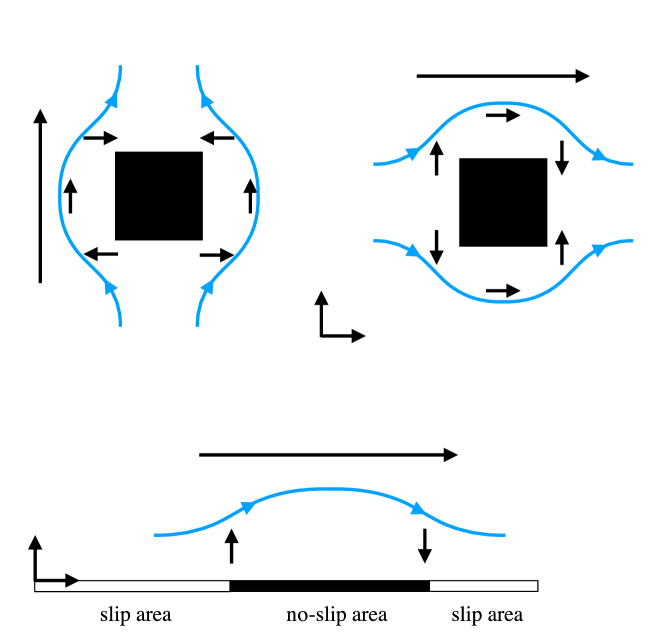
In general, however, the overlying flow induces a velocity field around texture elements in all three directions, while itself has also components in all three directions. The spanwise background flow would for instance induce a texture-coherent, spanwise . Therefore, all three texture-coherent velocity components would have contributions induced by all three components of the overlying flow, such that equation 5 would have additional terms for and , the streamwise velocities induced by the background and . To illustrate this idea, figure 1 shows a sketch of the streamwise and spanwise overlying velocities inducing coherent flow. Applied to all velocity components, the amplitude-modulated triple decomposition of Abderrahaman-Elena et al. (2019) can be written as the product of a matrix and a vector,
overlying streamwise velocity, overlying spanwise velocity, overlying streamwise (cf. spanwise) velocity (cf. ) (cf. ) (cf. )
| (6) |
where and denote the direction-conditional averages of and over individual roughness elements, thus giving a norm for the intensity of the respective texture-coherent velocities. Abderrahaman-Elena et al. (2019) showed that this modified form of the triple decomposition was more effective at removing the footprint of the texture from .
2.2 Governing equations for the background turbulence in flows over textures
Let us now derive the governing equations for the background-turbulence component, and in particular the terms that account for the non-linear interaction with the texture-coherent flow. In a texture-resolving DNS, the incompressible flow within the channel is governed by continuity, , and the Navier-Stokes equations,
| (7) |
where is the velocity vector with components , , . Using the velocity decompositions introduced in section 2.1, the governing momentum equations for the background turbulence can be derived by subtracting the momentum equation for texture-coherent flow from the triple-decomposed Navier-Stokes equations. We apply this first for the case of conventional triple decomposition, as a simpler example that serves us to illustrate the concept, and then apply it for the case of amplitude-modulated decomposition.
2.2.1 Texture-coherent flow obtained from conventional triple decomposition
Using conventional triple decomposition, the velocity vector can be written as
| (8) |
and the pressure as , where is the contribution that provides the mean pressure gradient driving the flow. Substituting the triple-decomposed velocities and pressure into the Navier-Stokes equations and taking the temporal and spatial average, we obtain the momentum equation for the mean flow ,
| (9) |
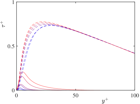
where denotes spatial averaging in the wall-parallel directions and denotes temporal averaging. This has the usual form of the mean-flow equation for rough-wall flows, with the Reynolds and the dispersive stress on left hand side. While the dispersive stress can be significant for other textures, for the present slip/no-slip textures it is negligible compared to the Reynolds stress at least for , only becoming relevant for texture sizes , as shown in figure 2.
The momentum equation for the texture-coherent fluctuation, , can be obtained by taking the temporal average of the triple-decomposed Navier-Stokes equations and subtracting the momentum equation for , equation 9, which gives
| (10) |
where
| (11) |
Given that the background turbulence is homogeneous in the wall-parallel directions and statistically steady in time, we have in the non-linear term , and the resulting momentum equation for the texture-coherent fluctuation, , simplifies then to
| (12) |
Finally, the momentum equation for the background turbulence can be obtained by subtracting the above momentum equation for from the full triple-decomposed Navier-stokes equation, yielding
| (13) |
where includes the mean profile and the background turbulent fluctuations, and is thus the flow we are interested in solving for in our texture-less DNSs, and is the corresponding background pressure, . The additional non-linear terms, , are
| (14) |
where are the non-linear interactions of the background turbulence and the texture-coherent flow and is the dispersive stress, which acts only on the mean flow . The presence of surface texture thus modifies the background turbulence through these non-linear terms.
2.2.2 Texture-coherent flow obtained from amplitude-modulated triple decomposition
Let us now derive the momentum equations for the background turbulence using the amplitude-modulated triple decomposition of equation 6. For the present case of slip/no-slip textures, we make the following simplifications. At the surface, the wall-normal velocity is zero throughout, and therefore any flow induced by the background is small, as reported in Fairhall et al. (2019), so we neglect , and in equation 6. Let us however note that this -induced flow could be important for protruding textures such as pyramids, cones, and roughness in general. In addition, we also neglect the flow induced by the background , since the latter is weak compared to the background streamwise flow for slip/no-slip textures, as also reported in Fairhall et al. (2019). The dominant texture-coherent effect is then the flow induced by streamwise velocity , and the modulated triple decomposition simplifies then to
| (15) |
where we assume that can still be obtained by ensemble averaging (Abderrahaman-Elena et al., 2019; Fairhall et al., 2019) and is therefore still governed by equation 10. Similarly, the pressure is decomposed into
| (16) |
which can be further written as
| (17) |
where , corresponding to a linear expansion about .
The Navier-Stokes equations can then be written as
| (18) |
Following the procedure in section 2.2.1, the momentum equation for the background flow can be obtained by subtracting the governing equation for texture-coherent flow, equation 10, from equation 18,
| (19) |
where
| (20) |
and
| (21) |
Here, we have drawn a parallel with the result using conventional triple decomposition of equation 13 by grouping the additional advective terms into , and any other additional terms arising from the amplitude modulation into a residual . In appendix A we report on the magnitude of the latter, and show that is the dominant term. We will thus neglect the residual in our model.
Finally, we can derive the momentum equation for the mean velocity analogously to equation 9 by taking the temporal average of equation 19 particularised for the Fourier - zero mode, that is, for the - spatial average. This gives
| (22) |
where the forcing term is
| (23) |
Here, has been rearranged as before averaging in time. Integrating the above mean momentum equation in gives the following stress balance
| (24) |
where the role of the dispersive Reynolds stress in equation 9 is now played by an extended term ,
| (25) |
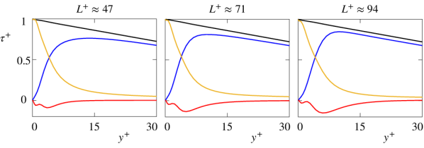
includes contributions from the background turbulence, and can thus only be calculated from the results in §4 a posteriori in order to verify that the sum of the three stresses in equation 24 is indeed linear. Results of such measurement are portrayed for reference in figure 3 for the collocated textures of sizes , as for smaller textures the contribution of is negligible. For the sizes portrayed its intensity increases with , although it remains small compared to the viscous and background Reynolds stress.
3 Numerical Method
To investigate the non-linear interaction between background turbulence and texture-coherent flow, direct numerical simulations (DNS) of turbulent channels were conducted. The numerical code is adapted from that of Fairhall et al. (2019), and is briefly summarised here. The three-dimensional incompressible Navier-Stokes equations are solved using a spectral discretisation in the streamwise and spanwise directions with the wall-normal direction discretised by second-order finite differences on a staggered grid. A fractional step method (Kim & Moin, 1985), combined with a three-step Runge-Kutta scheme, is used to advance in time, with a semi-implicit scheme used for the viscous terms and an explicit scheme for the advective terms (Le & Moin, 1991). The simulations were run with constant mean pressure gradients, adjusted to achieve the desired friction Reynolds numbers, Reτ. The channel is of size in the streamwise, spanwise and wall-normal directions respectively, where is the channel half-height. Once a statistically steady state was reached, statistics were obtained over 10 times the characteristic largest-eddy-turnover time, .
Three sets of DNSs were conducted. The first set consists of texture-resolving simulations with patterns of alternating regions of slip/no-slip boundary conditions on the channel walls. The first set used the DNS code from Fairhall et al. (2019) unmodified. The surfaces are assumed rigidly flat, which leads to zero transpiration. This is a widely used idealisation for superhydrophobic surfaces, where the free-slip regions represent the gas pockets, and the no-slip regions the exposed tips of solid posts. The assumption of free slip is reasonable if the gas pockets are sufficiently deep (Schönecker et al., 2014). The assumption of flat, rigid interfaces is reasonable for for typical applications (Seo & Mani, 2018). We note nevertheless that in this study we use this model to keep the surface texture as simple as possible, regardless of whether the model is a suitable representation or not of superhydrophobic textures. The latter question is out of the scope of this work.
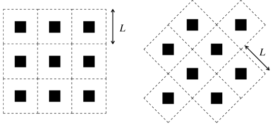
We consider texture elements consisting of periodic arrays of square posts, both in collocated and staggered arrangements, as illustrated in figure 4, with a solid fraction, the ratio of post area to total surface area, . The texture unit is a square of side , repeated periodically in the streamwise and spanwise directions. For our different simulations, the texture size ranges from 18 to 94 for the collocated textures and 33 to 66 for the staggered textures.
The second set of DNSs replaces the textured surfaces by their corresponding homogeneous slip lengths, obtained a posteriori from the corresponding texture-resolving simulations. This set also used the DNS code from Fairhall et al. (2019) unmodified. The last set of DNSs are homogeneous-slip simulations with added forcing terms, with the same slip boundary conditions of the second set. The governing momentum equations have the additional non-linear forcing terms introduced in section 2.2, with the texture-coherent velocities obtained from ensemble-averaging in the texture-resolving simulations.
In order to reduce the computational cost of the texture-resolving simulations, the code uses a multiblock layout, where the near-wall regions have finer grids compared to the channel centre. This is done in order to resolve fully not just the channel turbulence but also the texture-coherent flow, which typically requires higher resolution. In the blocks containing the walls, each texture element is resolved by grid points in the and directions. In the central block, the grid resolution is 8.8 and 4.4. The latter resolution is also used throughout in the simulations with homogeneous slip. In the wall-normal direction, the grid is stretched, with resolution 0.3 at the surfaces and 3 in the channel centre, and with the fine--- resolution blocks extending a height into the channel from the wall, which was verified a posteriori to exceed the height at which any fine, texture-induced flow became vanishingly small. Overall, this resulted for instance in roughly grid points for case TX18 or for TX47, which can be compared with for the corresponding smooth-wall and texture-less simulations, or for TX18 if uniform resolution in and had been applied throughout.
The texture-resolving and homogeneous-slip simulations with collocated elements with sizes to 47 are from Fairhall et al. (2019). Additional simulations with and 94, as well as the simulations with staggered elements, have been conducted to complete and expand the database. Simulations with homogeneous slip and added forcing have been conducted matching all the above cases to investigate the effect of the non-linear interaction. The parameters of all three sets of simulations are listed in table 1.
| Case | |||||||
| TX18 | 179.7 | 17.7 | 1576 | 768 | 5.8 | 4.0 | 3.7 |
| TX24 | 180.2 | 23.6 | 1152 | 576 | 6.9 | 4.3 | 4.1 |
| TX35 | 179.9 | 35.3 | 768 | 384 | 8.5 | 5.0 | 4.8 |
| TX35H | 407.0 | 35.3 | 1728 | 864 | 8.4 | 5.1 | 5.4 |
| TX47 | 180.1 | 47.1 | 576 | 288 | 10.0 | 6.3 | 5.6 |
| TX71 | 180.0 | 70.7 | 384 | 192 | 12.7 | 7.3 | 7.5 |
| TX94 | 179.7 | 94.2 | 288 | 144 | 14.6 | 8.5 | 9.1 |
| TX94H | 360.7 | 94.2 | 576 | 288 | 14.2 | 10.0 | 9.7 |
| sTX35 | 181.0 | 33.3 | 576 | 288 | 6.0 | 4.4 | 3.7 |
| sTX47 | 180.7 | 49.9 | 384 | 192 | 7.3 | 4.7 | 4.1 |
| sTX71 | 179.8 | 66.6 | 288 | 144 | 8.5 | 3.2 | 4.7 |
| SL18 | 179.9 | 17.7 | 128 | 128 | 5.8 | 4.0 | 4.0 |
| SL24 | 179.9 | 23.6 | 128 | 128 | 6.9 | 4.3 | 5.0 |
| SL35 | 180.3 | 35.3 | 128 | 128 | 8.5 | 5.0 | 6.5 |
| SL35H | 405.4 | 35.3 | 256 | 256 | 8.4 | 5.1 | 6.5 |
| SL47 | 179.7 | 47.1 | 128 | 128 | 10.0 | 6.3 | 7.8 |
| SL71 | 179.9 | 70.7 | 128 | 128 | 12.7 | 7.3 | 10.2 |
| SL94 | 179.9 | 94.2 | 128 | 128 | 14.6 | 8.5 | 12.1 |
| SL94H | 359.7 | 94.2 | 256 | 256 | 14.2 | 10.0 | 12.1 |
| sSL35 | 180.1 | 33.3 | 128 | 128 | 6.0 | 4.4 | 4.2 |
| sSL47 | 180.4 | 49.9 | 128 | 128 | 7.3 | 4.7 | 5.3 |
| sSL71 | 180.0 | 66.6 | 128 | 128 | 8.5 | 3.2 | 6.9 |
| FA18 | 179.9 | 17.7 | 128 | 128 | 5.8 | 4.0 | 3.6 |
| FA24R | 180.1 | 23.6 | 128 | 128 | 6.9 | 4.3 | 4.8 |
| FA24 | 180.0 | 23.6 | 128 | 128 | 6.9 | 4.3 | 4.0 |
| FA24S | 180.2 | 23.6 | 128 | 128 | 6.9 | 4.3 | 4.0 |
| FA35R | 180.1 | 35.3 | 128 | 128 | 8.5 | 5.0 | 6.0 |
| FA35 | 179.8 | 35.3 | 128 | 128 | 8.5 | 5.0 | 4.8 |
| FA35S | 180.0 | 35.3 | 128 | 128 | 8.5 | 5.0 | 5.0 |
| FA35H | 404.7 | 35.3 | 256 | 256 | 8.4 | 5.1 | 5.4 |
| FA47R | 180.3 | 47.1 | 128 | 128 | 10.0 | 6.3 | 7.0 |
| FA47 | 180.2 | 47.1 | 128 | 128 | 10.0 | 6.3 | 5.7 |
| FA71R | 180.0 | 70.7 | 128 | 128 | 12.7 | 7.3 | 8.9 |
| FA71 | 180.1 | 70.7 | 128 | 128 | 12.7 | 7.3 | 7.9 |
| FA94R | 179.9 | 94.2 | 128 | 128 | 14.6 | 8.5 | 10.5 |
| FA94 | 180.0 | 94.2 | 128 | 128 | 14.6 | 8.5 | 9.9 |
| FA94H | 359.5 | 94.2 | 256 | 256 | 14.2 | 10.0 | 10.2 |
| sFA35 | 179.8 | 33.3 | 128 | 128 | 6.0 | 4.4 | 3.6 |
| sFA47 | 180.3 | 49.9 | 128 | 128 | 7.3 | 4.7 | 4.1 |
| sFA71 | 180.1 | 66.6 | 128 | 128 | 8.5 | 3.2 | 5.4 |
3.1 Dealiasing for the forcing terms
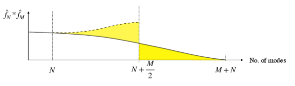
When calculating the product of two variables, such as in the advective term, in discrete Fourier space, the problem of aliasing arises. The convolution of two discrete functions, and , containing and discrete modes, results in a function containing modes. However, if the product function allocated for the convolution, , is of size , the excess modes cannot be correctly represented. This additional, high frequency information is then reflected into the resolved modes of the product function.
The method typically used to address this aliasing is to pad and with additional modes, with zero value, before the multiplication (Canuto et al., 2012). For the non-linear term in equation 14, we use the standard ‘2/3 rule’ for dealiasing. All functions have the same size, , so they need to be padded with an additional modes to prevent aliasing in in modes 0 to . Aliasing still occurs from the reflection of modes greater than into modes from to , but this is of no consequence as these modes are discarded once the convolution product has been calculated. In contrast with the standard advection, for the product , the convolution of the background turbulence and the texture-coherent flow, the sizes of the two components need not be the same. We have for instance for , with different for cases with different texture size, and typically . Since we are interested in solving only the background turbulence, that is, modes up to , for dealiasing in this case we need at least , as illustrated in figure 5. Taking case FA35 as an example, in the streamwise direction the texture-coherent component has points in discrete Fourier space, so is required for dealiasing.
4 Results and discussion
In this section, we present and discuss the results of the DNSs summarised in table 1. We first compare the drag predictions obtained from simulations with the texture resolved and those with its effect modelled. Figure 6 portrays those results in terms of the velocity increment . For each simulation setup, the figure shows the usual increase of with texture size . The results with resolved textures and with the corresponding slip boundary conditions agree well only up to texture sizes (for smaller textures see results in Fairhall et al., 2019) for collocated layouts and for staggered ones, although we note that the streamwise spacing between successive rows of posts is then , close to the collocated value. For larger spacings, using the equivalent homogeneous slip increasingly overpredicts , by % for in the case of collocated posts, and by a similar proportion for staggered ones. This difference was already reported by Fairhall et al. (2019). They argued that, given that the effective boundary conditions perceived by the overlying turbulence were the same for texture-resolved and slip simulations, the difference in drag had to arise from differences in the overlying flow. Introducing the forcing terms without amplitude modulation from §2.2.1 improves the prediction of for slip-only simulations partially, as shown in Figure 6. The error remains however large, and is only reduced by 30–50%. In turn, introducing the forcing terms with amplitude modulation from §2.2.2 yields values of in good agreement with those of texture-resolved simulations at least up to texture sizes . As the texture size increases further to , the results begin to depart. Although the deviation remains below 10%, we already expected the forcing model to break down in this range of , as the assumption gradually ceases to hold that there is sufficient separation of scales between the overlying shear and the texture-coherent flow it induces, rendering the flow decomposition used in the forcing model invalid. This is further discussed in §4.1.
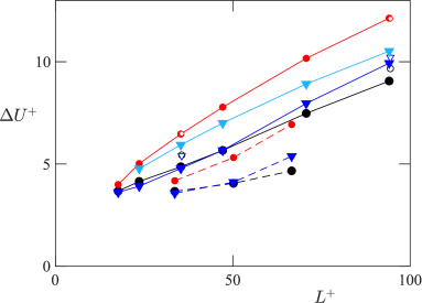
For the staggered-posts layouts, the values of are lower than for collocated layouts with the same . This is in agreement with the Stokes-flow predictions for small textures of Sbragaglia & Prosperetti (2007). They argued that collocated textures channel the flow through streamwise-aligned channels between posts, while staggered arrangements obstruct this channelling effect, reducing the mean slip velocity. This obstruction was also important in the simulations of Seo & Mani (2018), who observed that the slip lengths measured from DNSs of surfaces with randomly distributed texture elements was reduced by approximately 30% compared to collocated elements. In any event, the results for texture-resolved, slip-only and slip-plus-forcing simulations for staggered posts follow generally the same trends observed for collocated posts, albeit with lower values of for the same , and are therefore not presented in the remainder of this section. They are nevertheless included for completeness in appendix B.
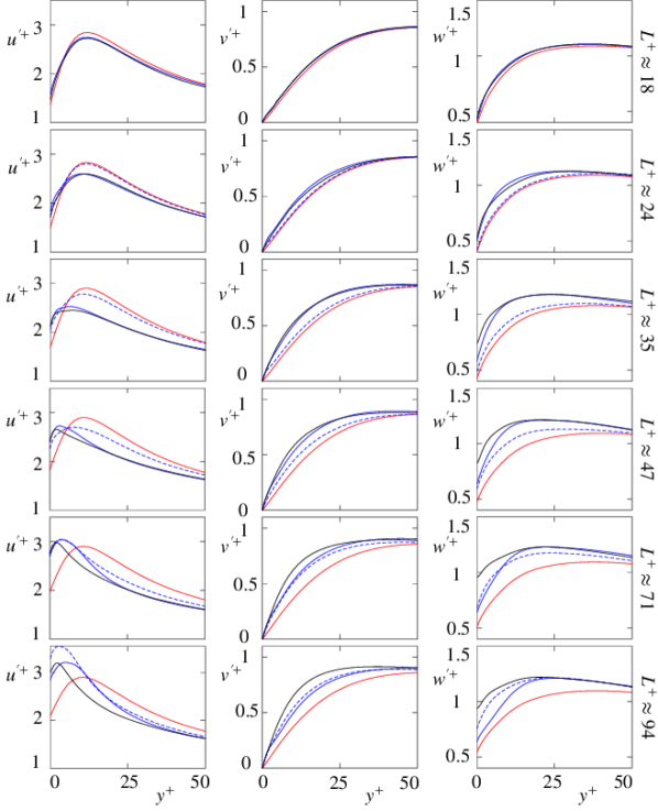
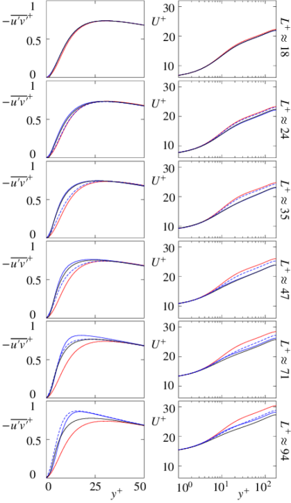
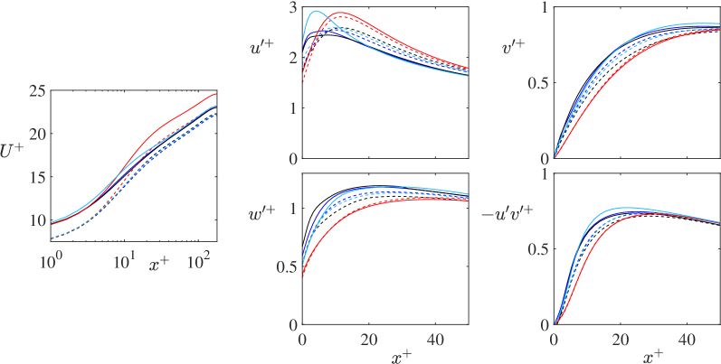
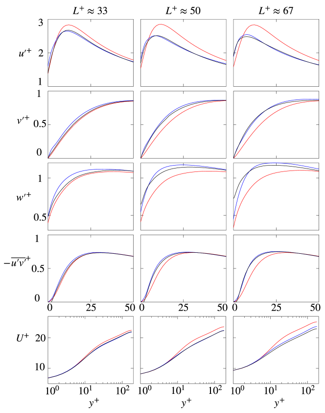
The agreement exhibited by the roughness function between texture-resolved simulations and texture-less simulations with amplitude-modulated forcing extends to other flow properties. This is the case for instance of one-point turbulent statistics. Figures 7 and 8 portray the r.m.s. velocity fluctuations and the shear Reynolds stress and mean velocity profile for texture-resolved, slip-only and slip-plus-forcing simulations, both using amplitude-modulated and conventional triple decomposition, across the range –. For , even slip-only simulations show good agreement with fully resolved ones. This was reported by Fairhall et al. (2019) as the limit size for which slip-lengths alone could capture the effect of the texture, as the texture-coherent flow is small in amplitude and confined to the immediate vicinity of the surface, and does therefore not alter the background turbulence significantly. The latter remains then smooth-wall like, other than by a shift in apparent origins (Ibrahim et al., 2021). In agreement with this, adding forcing to model the effect of the texture-coherent fluctuations in this range has little effect and essentially does not alter the flow. As the texture size increases from , though, the flow begins to depart from the smooth-wall-like behaviour that slip boundary conditions yield, as shown in figures 7 and 8, with a decrease of the streamwise fluctuation intensity above , and an increase throughout of the spanwise and wall-normal intensities and of the shear Reynolds stress. We note that the latter is in all cases zero at the surface, a unique feature of slip-no slip textures caused by the zero transpiration at . In general, the above modifications, which tend to decay sufficiently away from the wall, roughly at 50, are observed over slip/no-slip textures (Seo et al., 2015; Fairhall et al., 2019) but also over rough surfaces (Orlandi & Leonardi, 2006; Abderrahaman-Elena et al., 2019).
The addition of forcing using conventional triple decomposition can reproduce some of the departures from smooth-wall-like flow mentioned above for textured simulations, but forcing with amplitude modulation shows much better agreement with the resolved-texture cases. The agreement is excellent up to and first begins to break down for the spanwise velocity. This was to be expected given the simplifications made in equation 15, and has little effect on the Reynolds stress and, therefore, on the mean velocity profile and the drag. The agreement breaks down further for , for which it begins to propagate into , although it is still reasonable. For the departures become significant. We therefore identify this as the limit beyond which the model proposed here fails.
As mentioned in section 1, the differences in the Reynolds stress profile shown in figure 8 are caused by the changes in the background turbulence. The latter are what the forcing models ultimately aim to capture. The increased Reynolds stress causes a downward shift of the mean velocity profile away from the wall, and a corresponding reduction in . This relationship can be quantified by integrating the streamwise momentum equation. Here we follow Gómez-de-Segura & García-Mayoral (2019). A first integral gives
| (26) |
where is the shear Reynolds stress, including any dispersive stress, and is the effective half-height of the channel, which accounts for the background turbulence perceiving a virtual origin at . Integrating equation 26 once more in the wall-normal direction, from the surface to a height sufficiently far above for all surface effects to have vanished, gives
| (27) |
where is the slip velocity, and is a simple function of , and . The same integral can be repeated for a reference smooth-wall flow at the same friction Reynolds number between the corresponding heights, and , yielding
| (28) |
where the subscript S denotes smooth-wall flow. The roughness function can then be obtained by subtracting equations 27 and 28,
| (29) |
For slip-only simulations, turbulence is smooth-wall like and the integral in equation 29 is essentially zero (Fairhall et al., 2019; Ibrahim et al., 2021). Near the wall, , so for we have . From equation 3, we have , so also . The roughness function reduces then to the offset between the apparent origins for the mean flow and for turbulence, (Luchini, 1996). For texture-resolved simulations, however, in addition to this origin offset, the increase in Reynolds stress causes further modifications to the mean velocity profile and the roughness function. Fairhall et al. (2019) observed that for the present slip/no-slip textures, with zero transpiration and dispersive stress at , the contribution from the latter to is negligible up to at least texture sizes , as shown in figure 2. Those modifications would then be essentially caused by changes in the background, texture-incoherent turbulence alone. Figure 8 shows that the forcing model with amplitude modulation is able to capture the effect of these changes on the Reynolds stress, and thus on , while the one with conventional triple decomposition captures those changes only partially.
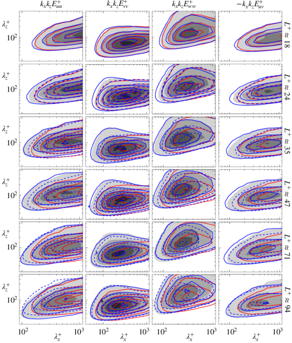
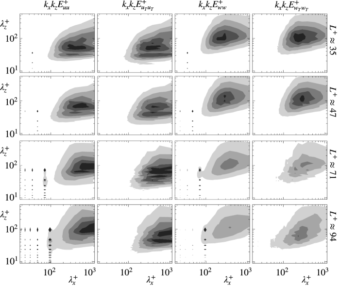
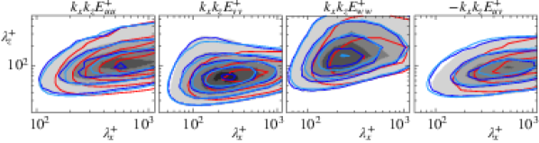
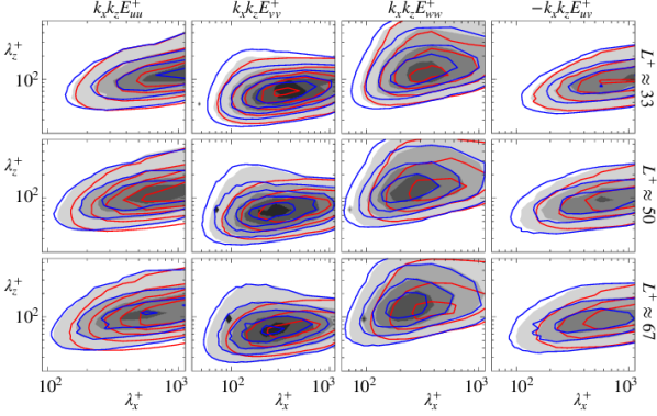
The modifications in the background turbulence can be observed in more detail in the spectral density maps of the different variables, as those portrayed in figure 9. Such maps show the contributions to the statistics shown in figures 7 and 8 at a given height from different streamwise and spanwise lengthscales. Figure 9 displays the energy densities at , a height of intense r.m.s. fluctuations of the background turbulence and also sufficiently above the surface for the texture-coherent flow to be negligible. As observed by Ibrahim et al. (2021), the signature of turbulence in slip-only simulations is essentially the same as over smooth walls. Compared to those cases, for fully resolved textures there is additional energy in shorter streamwise scales, and also in wider spanwise scales particularly for . This effect is negligible for , but becomes increasingly marked for greater . Figure 9 shows that slip-only models fail to capture this gradual change in the dynamics of the background turbulence for . The forcing model based on conventional triple decomposition is able to generate some additional energy in shorter and wider scales, but not to the full extent observed in texture-resolved simulations. In contrast, the forcing model based on amplitude modulation can generate energy in all the necessary scales, and results in a good overall collapse of the spectra with that for resolved textures up to . For larger , deviations appear first in the core regions of the maps for and and in streamwise long scales of and . These spectra indicate again that the additional forcing terms based on the amplitude-modulated decomposition can capture the effect of the texture on the background turbulence, while forcing based on conventional triple decomposition shows only a limited improvement compared to slip-only simulations.
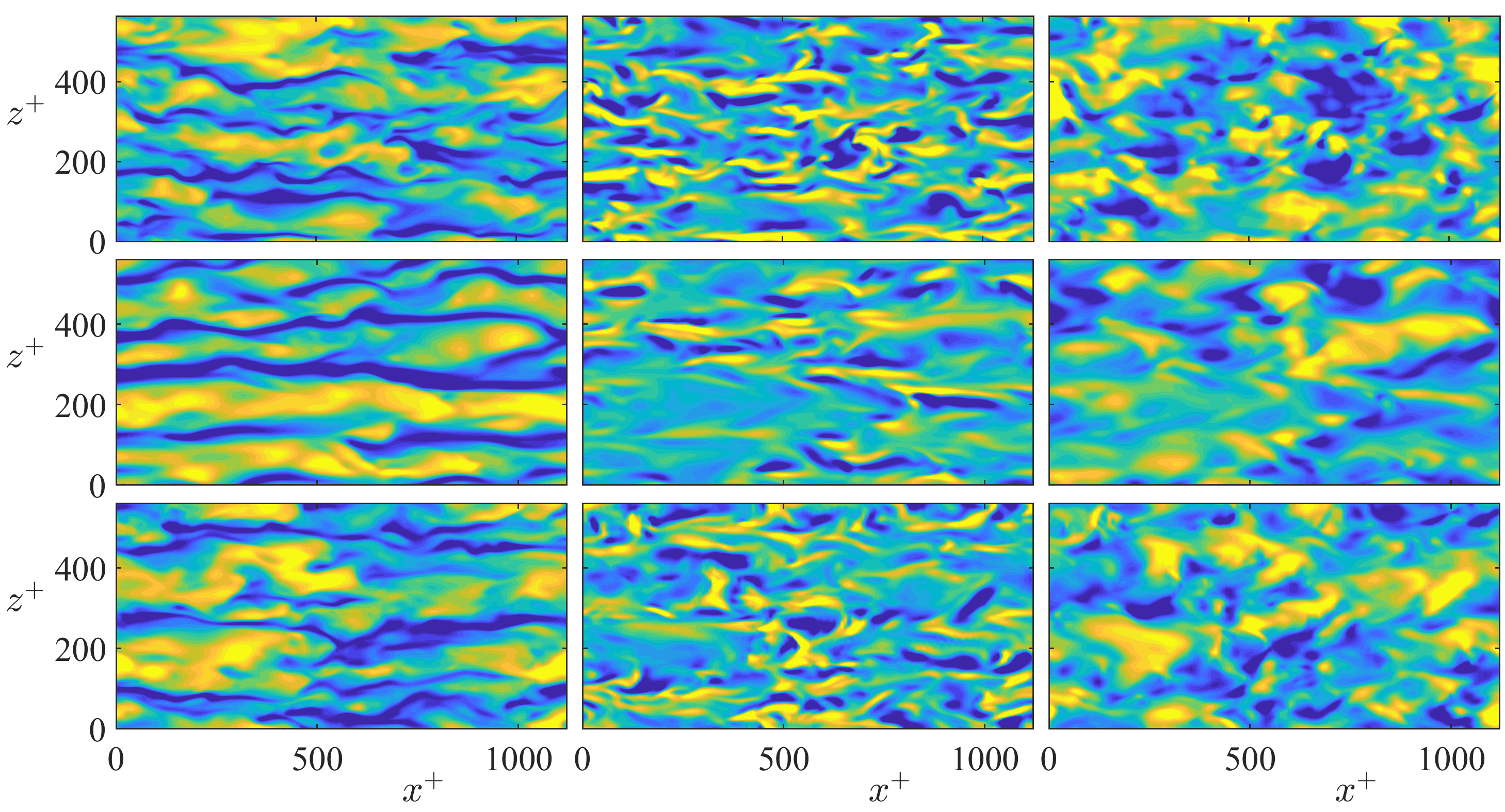
To illustrate the general appearance of the flow, instantaneous realisations of the three velocity components for texture-resolved, slip-only, and amplitude-modulated-forcing simulations are shown in figure 10 at a height for texture size . This size is large enough to exhibit significant differences across models, yet not so large that the forcing model begins to fail. While the slip-only simulation exhibits canonical, smooth-wall-like-turbulence structures, both the texture-resolving and the forcing-model simulations show a similar disruption of the latter, with a reduction in the coherence of the streamwise velocity for scales of order 1000 wall units, as indicated also by the energy spectra. For the wall-normal and spanwise velocities, the lengthscales of the turbulent eddies are also shorter compared to those over homogeneous slip. At this , the lengthscales and magnitude of the texture-coherent flow near the wall become comparable to those of the background turbulence. The spectra and instantaneous flow fields suggest a modification of the near-wall dynamics through the disruption of streaks and quasi-streamwise vortices by this texture-coherent flow. The similarity of the amplitude-modulated-forcing flow field and the texture-resolved one suggests that the alteration of the background turbulence by the presence of the texture can also be captured by the forcing model.
Finally, to verify that the expected scaling in viscous units for textures whose effect is confined to the vicinity of the wall (García-Mayoral & Jiménez, 2012) also holds for the corresponding models, in addition to the simulations at we have conducted simulations at for the collocated textures of size and . The results support this scaling, and are presented and discussed in appendix C.
4.1 The limit of the forcing model
The preceding discussion has shown how the model based on the amplitude-modulated decomposition works well up to , and how for and deviations from the fully resolved simulations are increasingly apparent. We have also mentioned that this is to be expected, as the assumption of separation of scales between the two flow components ceases to hold. The decomposition hinges on the idea that one component, the overlying background turbulence, excites the other, the texture-coherent signature, as the response flow in the immediate vicinity of the texture, which does not necessarily cease to hold once the lengthscales of the two become comparable. The algebraic form, however, as laid out in equation 5 or more generally in equation 6, assumes that the exciting overlying flow is on a much larger scale than the excited one, in the spirit of Luchini et al. (1991). As increases, the breakdown of scale separation occurs first for the cross flow components, as these are mainly produced by the overlying quasi-streamwise vortices, with length and span of order wall units, while the streamwise component is mainly produced by the streamwise streaks, with length and span of order wall units (Kline et al., 1967; Blackwelder & Eckelmann, 1979; Smith & Metzler, 1983).
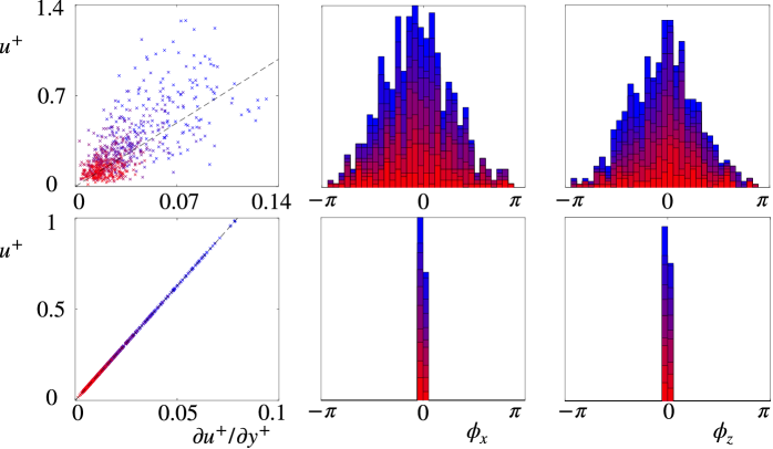
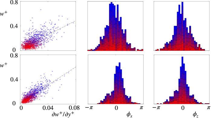
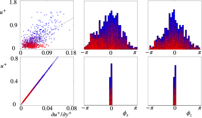
This difference can be observed in the earlier loss of correlation at the wall between velocity and shear in the spanwise direction. Fairhall et al. (2019) showed that the correlation held well for the background turbulence up to for both and . Figures 12 to 14 extend their analysis to the textures of size and . The figures show that the decomposition using equation 6 still results in an excellent recovery of the correlation between and for both texture sizes, both in terms of proportion and phase between them, which makes the value of estimated from this data meaningful. The same is however not true for the correlation between and , which exhibits a considerable scatter both in terms of phase and magnitude. As a result, it is difficult to define a spanwise slip length meaningfully. We note nevertheless that this is of minor importance with regards to setting the effective boundary condition for . At these large texture sizes, we have , and thus the effect of the slip length in the boundary condition for in equation 3 is significantly saturated, with variations in not resulting in significant variations in . In any event, the loss of correlation is indicative of the background turbulence component obtained still being contaminated by some amount of texture-induced signal, and thus of the decomposition produced using equation 6 breaking down.
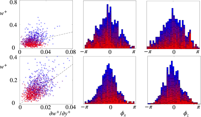
This breakdown is perhaps even clearer in the spectral densities of the tangential velocity components in the immediate vicinity of the texture, both for the background turbulence and the full texture-resolved flow, as portrayed at in figure 15. Up to texture size the main energetic region that can be observed in the spectra of and is recovered in the spectra of the background-turbulence components. However, for , the decomposition can successfully filter out the contributions in the vicinity of the texture harmonics, which is fully attributable to the texture-coherent flow and its modulation in amplitude (Abderrahaman-Elena et al., 2019; Fairhall et al., 2019), but the spectral signature of the background turbulence is visibly altered by the decomposition. This is indicative of equation 6 failing to produce the correct signal for the background turbulence in the latter size range. Figure 15 shows that this happens once the lengthscales of the harmonics induced by the texture begin to overlap significantly with the main spectral region of the background turbulence, that is, once scale separation ceases to hold.
The results for texture sizes portrayed in figures 6 to 9 indicate that the deviations from the texture-resolved results first occur for , and soon extend to the other velocity components. The contribution of long structures of and is particularly overpredicted, ultimately leading to an overprediction of the shear Reynolds stress and an underprediction of the drag. We note however that, even at , the amplitude-modulated model performs significantly better than the state-of-the-art slip-only models, even if they fail to capture fully the dynamics at play in texture-resolved simulations.
The present break down of the model for does not completely rule out its applicability for larger textures, and rather limits its validity in the present form of equations 15 and 19. It is entirely possible that a formulation of the flow decomposition not requiring scale separation could extend its validity to larger sizes. The present formulation also neglects any texture-coherent flow induced by cross-plane fluctuations. Such contributions to the texture-coherent flow would become increasingly important for larger texture sizes, leading to additional cross-advective forcing terms on the background turbulence. Their absence from the present formulation likely also contributes to its breakdown. Dropping the above simplifications would lead to a significantly more complex formulation, however, and is left for future work.
4.2 Using a priori estimates for the texture-coherent flow
The amplitude-modulated forcing model proposed in this paper shows good agreement with texture-resolved simulations at least up to texture sizes , both in terms of drag prediction and turbulent statistics and structure. This strongly suggests that the model has successfully identified the key physical mechanisms at play, i.e. the non-linear interactions between the texture-coherent flow and the background turbulence, and is able to reproduce them without resolving the texture elements. Our central aim in the present work was to identify and understand this mechanism, but ultimately it would also be interesting to use this understanding to design predictive tools. The results presented thus far do not have a truly predictive character, as they require a posteriori information on the texture-coherent flow obtained by ensemble averaging of texture-resolved simulations. In order to be fully predictive, the model would instead need a priori estimates of the texture-coherent flow. Such estimates are readily available, and their use is discussed below. The results are good, but we note, however, that this does not add to the understanding of the physical mechanism, and its usefulness as a predictive tool is somewhat limited, as it would still require running DNS-resolution simulations, even if without the texture-related resolution requirements. This is nevertheless a useful first step for the development of future models that circumvent the need for DNS altogether.
As mentioned in §1, Abderrahaman-Elena et al. (2019) observed that the ensemble average flow over small textures resembles the flow induced by a steady homogeneous overlying shear at matching , which can be obtained from laminar steady simulations of a single periodic unit of texture. This is in essence an extension of the Stokes-flow computations used by Luchini et al. (1991), Kamrin et al. (2010) and Luchini (2013) to predict protrusion heights or slip lengths, with the addition of inertial terms. The laminar computations of Abderrahaman-Elena et al. (2019) were extended for the slip/no-slip textures considered in this paper in Adams (2021). In the latter, a synthetic eddy-viscosity obtained from smooth-wall DNS was added to represent the effect of the background turbulence on the shape of the mean velocity profile under a driving pressure gradient. This eddy viscosity was essentially used so that the laminar computations yielded mean profiles more realistic than Couette or Poiseuille ones, although this only had a marginal effect on the texture-coherent flow, in its weaker regions away from the surface. It is analogue to a Van Driest (1956) or Cess (see Reynolds & Tiederman, 1967) conventional model, but was used instead because the latter was found to produce a poor surrogate for the smooth-wall profile at our low . Compared to the texture-resolved DNSs of Fairhall et al. (2019), the resulting flow fields for overpredicted the coherent by roughly 20%, and showed good agreement in and , yielding overall a reasonable estimate for the texture-coherent flow.
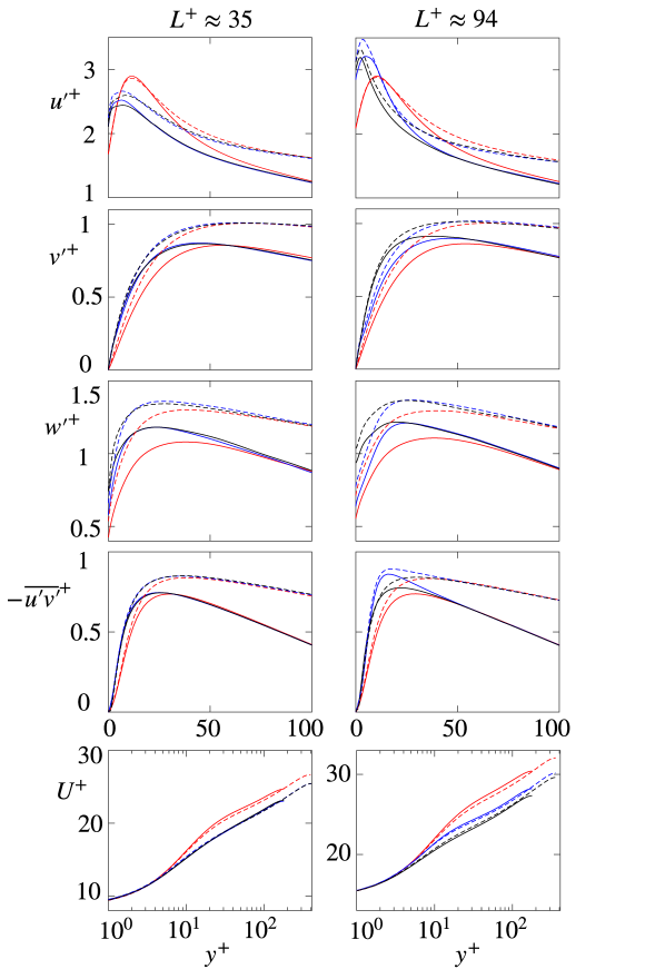
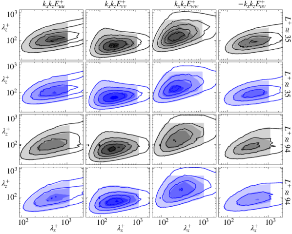
As a first step to explore the predictive capabilities of the amplitude-modulated forcing model, we study its performance when the texture-coherent flow from DNSs is replaced by the a priori surrogates of Adams (2021) for and . Results are shown in figures 16 and 17. Figure 16 shows excellent agreement in the r.m.s. velocity fluctuations, the Reynolds shear stress and , except for an overshoot in for the larger texture in the immediate vicinity of the wall, . This is likely caused by the excessive intensity in in the surrogate texture-coherent flow, as mentioned above. The overshoot does nevertheless not propagate into the Reynolds stress or any of the other velocity components, and is also confined to a narrow region near the texture, so it essentially does not alter the drag or the near-wall dynamics and dissipation, mainly governed by cross-plane velocities induced by bursts and quasi-streamwise vortices (Ibrahim et al., 2021; Habibi Khorasani et al., 2022; Jiménez, 2022). Similar results can also be observed in the spectral densities, shown for the three velocity components and the Reynolds shear stress at in figure 17 for . The surrogate texture-coherent flow is able to produce an energetic signature in the same short wavelengths exhibited by texture-resolved simulations and those with forcing based on the a posteriori texture-coherent flow, and not present for smooth-wall or slip-only simulations. Although there is room for improvement, especially in the prediction of the near-wall peak in , these results suggest that the need to conduct simulations that resolve the texture can be fully circumvented, and that it is possible to resolve the background turbulence, and predict the drag and other flow properties using only a priori data on the texture detail, significantly reducing computational costs.
5 Conclusions
The simulation and prediction of turbulence over textured surfaces requires a spatial resolution that can be more demanding than that needed to resolve the turbulence itself, and can become prohibitive for texture sizes in the range -. This is a relevant range for applications, and includes the working range for drag-reducing textures and the transitionally rough range for drag-increasing ones, beyond which the effect on drag usually asymptotes. In this paper we have investigated the effect of the texture detailed geometry on the background turbulence, with the ultimate aim to sidestep the need to resolve that geometry directly. As a first approach, we have focused on a particularly simple, idealised texture, consisting of a slip/no-slip pattern on an otherwise flat surface, a popular model for superhydrophobic surfaces. Such slip/no-slip textures have some unique properties that simplify their analysis, namely that the effective boundary conditions for the overlying turbulence are well known and characterised, reducing to slip, Robin conditions for the tangential velocities and zero transpiration; and that the wall-normal velocity and Reynolds stress are zero at the reference, interfacial plane, and remain negligible in its vicinity. This allowed Fairhall et al. (2019) to identify that drag degraded due to additional Reynolds stresses occurring above the surface, rather than arising at the surface and propagating into the flow above. They proposed that such Reynolds stresses had to originate from the non-linear interaction of the texture-coherent flow with the background turbulence. This interaction became significant and could not be neglected for , and would need to be accounted for in any model in addition to the effective slip boundary conditions, which still held up in this range of sizes and at least up to ,
Following up from Fairhall et al. (2019), we have analysed how the decomposition of the flow into a texture-coherent and a background-turbulence components propagates into the governing equations of the two components separately. We have first decomposed the flow using conventional triple decomposition, which produces a much simpler set of governing equations. However, as observed by Abderrahaman-Elena et al. (2019), this decomposition results in a residual texture-coherent signature in the background turbulence. To separate fully the texture-coherent signal and obtain a texture-incoherent background turbulence, Abderrahaman-Elena et al. (2019) proposed a decomposition in which the latter modulates in amplitude the former. Here we have analysed the governing equations for the background turbulence that result from this decomposition. For both the conventional and the amplitude-modulated triple decomposition, we have argued that the background turbulence is governed by Navier-Stokes equations with additional, forcing terms, arising from the cross advective terms between both flow components.
To assess the above hypothesis, we have conducted a series of simulations in which the background turbulence was fully resolved, but the texture was replaced by the corresponding effective boundary conditions plus the forcing terms in the momentum equations mentioned above. For the formulation based on conventional triple decomposition, the results are partially improved compared to using effective boundary conditions alone. For the formulation based on the amplitude-modulated decomposition, the results show excellent agreement up to texture sizes , and begin to deviate for . This is the case both for the prediction of drag and , and for the statistical properties of turbulence, including r.m.s. velocity fluctuations, Reynolds stresses and mean velocity profiles. In particular, the addition of forcing terms can accurately generate fluctuations at shorter wavelengths than smooth-wall flows, which are present for geometry-resolved simulations but which the effective boundary conditions are unable to generate on their own. Once deviations begin to occur, for texture sizes , they first manifest in the spanwise velocity component. This is also the component for which the flow decomposition first begins to break down, likely due to the span of background-turbulence eddies becoming comparable to the texture size earlier than their length, which disrupts the implicit assumption of separation of scales embedded in the amplitude-modulated decomposition. Concurrently, the texture-coherent motions excited not only by the overlying streamwise velocity, but by the cross velocity components, cease to be negligible, and therefore our simplifications in the forcing also cease to hold.
The above results strongly suggest that the key effects of surface texture on the overlying turbulence are imposing a set of effective boundary conditions but, critically, also altering the momentum equations through the non-linear interaction with the texture-coherent flow in the advective terms. While this is useful in terms of identifying physical mechanisms, it falls short in terms of predictive power, as quantifying that interaction requires prior knowledge of the texture-coherent flow, but the latter only becomes available from the postprocessing of fully resolved flows. We have therefore also explored the possibility of using a priori surrogates for the texture-coherent flow, based on the laminar steady flow about a single periodic unit of texture. Preliminary results show good agreement, motivating further work.
The present study has only considered a particularly simple type of surface texture. The results are encouraging, but would need to be further tested in more complex and general textures, mainly roughness. Many of the simplifications possible here, e.g. the effective boundary conditions reducing to homogeneous slip and zero transpiration, or accounting only for the texture-coherent flow induced by the overlying streamwise velocity, will likely not apply in the general case, calling for a more complete and complex framework.
[Acknowledgements] Computational resources were provided by the University of Cambridge Research Computing Service under EPSRC Tier-2 grant EP/P020259/1, and by the UK ’ARCHER2’ system under PRACE (DECI-17) project pr1u1702 and EPSRC project e776. For the purpose of open access, the authors have applied a Creative Commons Attribution (CC BY) licence to any Author Accepted Manuscript version arising from this submission.
[Declaration of interests]The authors report no conflict of interest.
[Author ORCIDs]
Chris Fairhall, https://orcid.org/0000-0002-2529-3650;
R. García-Mayoral, https://orcid.org/0000-0001-5572-2607.
Appendix A Magnitude of the forcing term and the residual in the momentum equations
This appendix portrays evidence of the relative importance of the forcing term and the residual in equation 19. The residual is neglected in the governing equations of the simulations presented in §4 with forcing based on the amplitude-modulated decomposition, and it therefore needs to be small for the proposed model to hold. Conversely, if the magnitude of was small, we would expect that retaining this term had little effect on the dynamics of the background turbulence.
Figures 18 to 20 portray the time-r.m.s. magnitude of the different terms in equation 19 from the texture-resolved simulation of collocated posts with texture size (case TX35). Figures 18, 19 and 20 portray results for the streamwise, wall-normal and spanwise components of the momentum equation respectively, for a representative set of - wavenumbers and as a function of height . The figures show that the dynamics are mostly dominated by the interplay between temporal and advective terms, but in the vicinity of the wall, for , the forcing term, which is neglected in slip-only simulations, can become comparable to, and even larger that, the latter two. This is particularly the case for the streamwise momentum equation, as illustrated by figure 18, and across the whole range of wavelengths. For the spanwise and wall-normal momentum equations, the explicit contribution of appears to be less significant. In turn, the residual is also negligible in the spanwise and wall-normal momentum equations. It is typically a fraction of of order 1/4-1/3 in the streamwise one, and thus reasonably smaller than the leading-order terms. These results back up neglecting when implementing the amplitude-modulated forcing model in §4.
Appendix B Simulations for staggered-posts textures
Figures 21 and 22 portray results from the simulations for staggered-posts configurations, as sketched in figure 4. The aim of these simulations was to verify if the forcing model using amplitude-modulated decomposition, first tested for a collocated-posts texture, would also be applicable to other surface arrangements. In additions to simulations fully resolving the texture and simulations with forcing, we have also conducted simulations implementing slip boundary conditions alone, to serve as a benchmark for comparison. These simulations complement and expand the data set of Fairhall et al. (2019).
We have conducted simulations for texture sizes , and , aiming to span the size range for which slip-only simulations begin to deviate from texture-resolved ones, yet the texture size is not large enough for the decomposition and the forcing model to break down. The simulation parameters and resulting roughness functions are listed in table 1.
The results follow the same trends of the collocated-textures cases. Figure 21 shows that the r.m.s. velocity fluctuations for texture-resolved simulations exhibit differences with the slip-only ones, which display smooth-wall-like turbulence (Fairhall et al., 2019; Ibrahim et al., 2021). These differences are small for , but become increasingly pronounced for larger texture sizes. Their most salient features are a decrease in near-wall peak and an increase in and . These differences eventually result in a significant increase in the shear Reynolds stress, and a corresponding downward shift of the mean velocity profile away from the wall. The forcing model is able to accurately capture these differences, and produces results very close to those of texture-resolved simulations, with small deviations first appearing in , as discussed in §4 for collocated textures.
The spectral densities portrayed in figure 22 are also consistent with the observations in §4 for collocated textures. Compared to smooth-wall turbulence, in texture-resolving simulations have additional energy particularly in shorter scales in the streamwise direction. Slip-only simulations are not able to produce this modification in turbulence, and their spectrum remains essentially smooth wall like as discussed in Fairhall et al. (2019) and Ibrahim et al. (2021). In contrast, the forcing model is able to produce the spectral energy densities of texture-resolved simulations with excellent agreement.
Appendix C Effect of Reynolds number
The main set of simulations discussed in this paper were conducted at . To verify that our observations would scale out to other Reynolds numbers, we have conducted a reduced set of simulations at , otherwise matching in inner scaling setups from the main set, with results shown in figures 23 and 24. We have chosen the collocated layouts with and , as one texture size for which the texture-resolved and the forcing simulations show good agreement between them, but differences with the slip-only simulation, and one texture size for which the forcing model shows signs of breaking down.
The results are consistent with our usual observations for other surface topologies (García-Mayoral & Jiménez, 2012; Fairhall et al., 2019; Sharma & García-Mayoral, 2020a, b; Hao & García-Mayoral, 2024). Near the wall, the same effects are produced in inner units for matching simulations, with results eventually collapsing to smooth wall data at equal for . Differences in this region are observable, but entirely attributable to the variations in , as they are the same observed for smooth-wall flows (Moser et al., 1999). These are evidenced for instance in the higher peak levels of the r..m.s. velocity fluctuations and the shear Reynolds stress near , as shown in figure 23. The spectral densities portrayed in 24 confirm these results. The spectral energy content at each wavelength matches when scaled in inner units for corresponding simulations, with larger-scale content only resolved for the higher , as made possible by the larger simulation domain. Overall, the results suggest that the effect of the model, like the effect of the texture, scales in inner units as expected, and can be extrapolated to and used at different Reynolds numbers.
References
- Abderrahaman-Elena et al. (2019) Abderrahaman-Elena, N., Fairhall, C. T. & García-Mayoral, R. 2019 Modulation of near-wall turbulence in the transitionally rough regime. J. Fluid. Mech. 865, 1042–1071.
- Abderrahaman-Elena & García-Mayoral (2017) Abderrahaman-Elena, N. & García-Mayoral, R. 2017 Analysis of anisotropically permeable surfaces for turbulent drag reduction. Phys. Rev. Fluids 2 (11), 114609.
- Adams (2021) Adams, M. 2021 Laminar models for the dispersive flow in turbulence over superhydrophobic surfaces. Tech. Rep.. University of Cambridge.
- Blackwelder & Eckelmann (1979) Blackwelder, Ron F. & Eckelmann, Helmut 1979 Streamwise vortices associated with the bursting phenomenon. J. Fluid Mech. 94 (3), 577–594.
- Bottaro (2019) Bottaro, A. 2019 Flow over natural or engineered surfaces: an adjoint homogenization perspective. J. Fluid Mech. 877.
- Busse & Sandham (2012) Busse, A. & Sandham, N. D. 2012 Influence of an anisotropic slip-length boundary condition on turbulent channel flow. Phys. Fluids 24, 055111.
- Canuto et al. (2012) Canuto, C., Hussaini, M. Y., Quarteroni, A., Thomas Jr, A. & others 2012 Spectral methods in fluid dynamics. Springer Science & Business Media.
- Cheng & Castro (2002) Cheng, H. & Castro, I. P 2002 Near wall flow over urban-like roughness. Bound.-Layer Meteorol. 104 (2), 229–259.
- Chung et al. (2021) Chung, D., Hutchins, N., Schultz, M. P. & Flack, K. A. 2021 Predicting the drag of rough surfaces. Annu. Rev. Fluid Mech. 53, 439–471.
- Clauser (1956) Clauser, F. H. 1956 The turbulent boundary layer. In Adv. Appl. Mech., , vol. 4, pp. 1–51. Elsevier.
- Coceal et al. (2007) Coceal, O., Dobre, A., Thomas, T. G. & Belcher, S. E. 2007 Structure of turbulent flow over regular arrays of cubical roughness. J. Fluid Mech. 589, 375–409.
- Colebrook & White (1937) Colebrook, C. F. & White, C. M. 1937 Experiments with fluid friction in roughened pipes. Proc. R. Soc. Lond. A - Math Phys. Sci. 161 (906), 367–381.
- Fairhall et al. (2019) Fairhall, C. T., Abderrahaman-Elena, N. & García-Mayoral, R. 2019 The effect of slip and surface texture on turbulence over superhydrophobic surfaces. J. Fluid Mech. 861, 88–118.
- Fairhall & García-Mayoral (2018) Fairhall, C. T. & García-Mayoral, R. 2018 Spectral Analysis of the Slip-Length Model for Turbulence over Textured Superhydrophobic Surfaces. Flow Turbul. Combust. 100, 961–978.
- García-Mayoral et al. (2019) García-Mayoral, R., Gómez-de-Segura, G. & Fairhall, C. T. 2019 The control of near-wall turbulence through surface texturing. Fluid Dyn. Res. 51, 011410.
- García-Mayoral & Jiménez (2011) García-Mayoral, R. & Jiménez, J. 2011 Hydrodynamic stability and breakdown of the viscous regime over riblets. J. Fluid Mech. 678, 317–347.
- García-Mayoral & Jiménez (2012) García-Mayoral, R. & Jiménez, J. 2012 Scaling of turbulent structures in riblet channels up to re. Phys. Fluids 24 (10), 105101.
- Gómez-de-Segura & García-Mayoral (2019) Gómez-de-Segura, G. & García-Mayoral, R. 2019 Turbulent drag reduction by anisotropic permeable substrates analysis and direct numerical simulations. J. Fluid Mech. 875, 124–172.
- Gómez-de-Segura & García-Mayoral (2020) Gómez-de-Segura, G. & García-Mayoral, R. 2020 Imposing virtual origins on the velocity components in direct numerical simulations. Int J Heat Fluid Flow 86, 108675.
- Habibi Khorasani et al. (2022) Habibi Khorasani, S. M., Lācis, U., Pasche, S., Rosti, M. E. & Bagheri, S. 2022 Near-wall turbulence alteration with the transpiration-resistance model. J. Fluid Mech. 942, A45.
- Hao & García-Mayoral (2024) Hao, Z. & García-Mayoral, R. 2024 Turbulent flows over porous and rough substrates, arXiv: 2402.15244.
- Ibrahim et al. (2021) Ibrahim, J. I., Gómez-de-Segura, G., Chung, D. & García-Mayoral, R. 2021 The smooth-wall-like behaviour of turbulence over drag-altering surfaces: a unifying virtual-origin framework. J. Fluid Mech. 915.
- Jelly et al. (2014) Jelly, T. O., Jung, S. Y. & Zaki, T. A. 2014 Turbulence and skin friction modification in channel flow with streamwise-aligned superhydrophobic surface texture. Phys. Fluids 26, 095102.
- Jiménez (2004) Jiménez, J. 2004 Turbulent flows over rough walls. Annu. Rev. Fluid Mech. 36, 173–196.
- Jiménez (2022) Jiménez, J 2022 The streaks of wall-bounded turbulence need not be long. J. Fluid Mech. 945, R3.
- Kamrin et al. (2010) Kamrin, K., Bazant, M.Z. & Stone, H.A. 2010 Effective slip boundary conditions for arbitrary periodic surfaces: the surface mobility tensor. J. Fluid Mech. 658, 409––437.
- Kim & Moin (1985) Kim, J. & Moin, P. 1985 Application of a Fractional-Step Method to Incompressible Navier-Stokes Equations. J. Comp. Phys. 59, 308–323.
- Kline et al. (1967) Kline, S. J., Reynolds, W. C., Schraub, F. A. & Runstadler, P. W. 1967 The structure of turbulent boundary layers. J. Fluid Mech. 30 (4), 741–773.
- Lācis & Bagheri (2017) Lācis, U. & Bagheri, S. 2017 A framework for computing effective boundary conditions at the interface between free fluid and a porous medium. J. Fluid Mech. 812, 866–889.
- Le & Moin (1991) Le, H. & Moin, P. 1991 An improvement of fractional step methods for the incompressible Navier-Stokes equations. J. Comp. Phys. 92, 369–379.
- Luchini (1996) Luchini, P. 1996 Reducing the turbulent skin friction. In Computational Methods in Applied Sciences – Proc. 3rd ECCOMAS CFD Conference, pp. 466–470.
- Luchini (2013) Luchini, P. 2013 Linearized no-slip boundary conditions at a rough surface. J. Fluid Mech. 737, 349–367.
- Luchini et al. (1991) Luchini, P., Manzo, F. & Pozzi, A. 1991 Resistance of a grooved surface to parallel flow and cross-flow. J. Fluid Mech. 228, 87–109.
- Min & Kim (2004) Min, T. & Kim, J. 2004 Effects of hydrophobic surface on skin-friction drag. Phys. Fluids 16, L55–L58.
- Moser et al. (1999) Moser, R. D., Kim, J. & Mansour, N. N. 1999 Direct numerical simulation of turbulent channel flow up to reτ=590. Phys. Fluids 11 (4), 943–945.
- Nikora et al. (2007) Nikora, V., McEwan, I., McLean, S., Coleman, S., Pokrajac, D. & Walters, R. 2007 Double-averaging concept for rough-bed open-channel and overland flows: Theoretical background. J. Hydraul. Eng. 133 (8), 873–883.
- Orlandi & Leonardi (2006) Orlandi, P. & Leonardi, S. 2006 Dns of turbulent channel flows with two- and three-dimensional roughness. J. Turbul. 7.
- Philip (1972) Philip, J. R. 1972 Flows Satisfying Mixed No-Slip and No-Shear Conditions. Z. Angew. Math. Phys. 23, 353–372.
- Reynolds & Tiederman (1967) Reynolds, W. C. & Tiederman, W. G. 1967 Stability of turbulent channel flow, with application to malkus’s theory. J. Fluid Mech. 27 (2), 253–272.
- Rothstein (2010) Rothstein, J. P. 2010 Slip on superhydrophobic surfaces. Annu. Rev. Fluid Mech. 42, 89–109.
- Sbragaglia & Prosperetti (2007) Sbragaglia, M. & Prosperetti, A. 2007 Effective velocity boundary condition at a mixed slip surface. J. Fluid Mech. 578, 435–451.
- Schlichting (1937) Schlichting, H. 1937 Experimental investigation of the problem of surface roughness. Tech. Rep. 823. NACA Tech. Mem.
- Schönecker et al. (2014) Schönecker, C., Baier, T. & Hardt, S. 2014 Influence of the enclosed fluid on the flow over a microstructured surface in the cassie state. J. Fluid Mech. 740, 168–195.
- Seo et al. (2015) Seo, J., García-Mayoral, R. & Mani, A. 2015 Pressure fluctuations and interfacial robustness in turbulent flows over superhydrophobic surfaces. J. Fluid Mech. 783, 448–473.
- Seo & Mani (2016) Seo, J. & Mani, A. 2016 On the scaling of the slip velocity in turbulent flows over superhydrophobic surfaces. Phys. Fluids 28, 025110.
- Seo & Mani (2018) Seo, J. & Mani, A. 2018 Effect of texture randomization on the slip and interfacial robustness in turbulent flows over superhydrophobic surfaces. Phys. Rev. Fluids 3 (4), 044601.
- Sharma & García-Mayoral (2020a) Sharma, A. & García-Mayoral, R. 2020a Scaling and dynamics of turbulence over sparse canopies. J. Fluid Mech. 888, A1.
- Sharma & García-Mayoral (2020b) Sharma, A. & García-Mayoral, R. 2020b Turbulent flows over dense filament canopies. J. Fluid Mech. 888, A2.
- Smith & Metzler (1983) Smith, C. R. & Metzler, S. P. 1983 The characteristics of low-speed streaks in the near-wall region of a turbulent boundary layer. J. Fluid Mech. 129 (1), 27–54.
- Spalart & McLean (2011) Spalart, P. R. & McLean, J. D. 2011 Drag reduction: enticing turbulence, and then an industry. Philos. Trans. R. Soc. A: Math, Phys. Eng. Sci. 369 (1940), 1556–1569.
- Türk et al. (2014) Türk, S., Daschiel, G., Stroh, A., Hasegawa, Y. & Frohnapfel, B. 2014 Turbulent flow over superhydrophobic surfaces with streamwise grooves. J. Fluid Mech. 747, 186–217.
- Van Driest (1956) Van Driest, E. R. 1956 On turbulent flow near a wall. J. Aeronaut. Sci. 23 (11), 1007–1011.
- Walsh & Lindemann (1984) Walsh, M. & Lindemann, A. 1984 Optimization and application of riblets for turbulent drag reduction. In 22nd aerospace sciences meeting, p. 347.