Restricted Regression in Networks
Abstract
Network regression with additive node-level random effects can be problematic when the primary interest is estimating unconditional regression coefficients and some covariates are exactly or nearly in the vector space of node-level effects. We introduce the Restricted Network Regression model, that removes the collinearity between fixed and random effects in network regression by orthogonalizing the random effects against the covariates. We discuss the change in the interpretation of the regression coefficients in Restricted Network Regression and analytically characterize the effect of Restricted Network Regression on the regression coefficients for continuous response data. We show through simulation with continuous and binary response data that Restricted Network Regression mitigates, but does not alleviate, network confounding, by providing improved estimation of the regression coefficients. We apply the Restricted Network Regression model in an analysis of 2015 Eurovision Song Contest voting data and show how the choice of regression model affects inference.
Keywords: network regression, confounding, restricted spatial regression, random effects
1 Introduction
Network data are measurements about the relationships between pairs of entities. These network measurements can be visualized as measurements on the edges between nodes of a graph (Becker et al.,, 1995). Examples of network data include relationships between potential borrowers on peer-to-peer lending platforms (Lee and Sohn,, 2022) or annual migration between countries (Aleskerov et al.,, 2017). Data are typically represented as a matrix, , where is the value in row and column , for . The value is the measurement about the dyadic relationship between the sending node and the receiving node . If for all , then the network is called undirected, otherwise it is called directed.
Network regression uses covariates measured on the node pairs to model the dyadic relationships. An example of such a model is
| (1) | ||||
| (2) |
where is the observed network measure, is a function mapping latent continuous values, , to the observed , is a -vector of covariates related to node , node or the relationship from node to node , is a -vector of regression coefficients, and is random error. For a binary observation indicating the presence or absence of an edge from node to node , a probit version of (1) is given by setting
| (3) | ||||
| (4) |
where the function is the indicator function (Albert and Chib,, 1993). For the rest of this paper, we will use to refer to a continuous latent variable resulting from the regression equation, and to refer to observations related to through a function, , possibly the identity function.
Network regression has found applications in medical meta-analysis (e.g., Li et al.,, 2018; Gwon et al.,, 2020), analysis of international politics (e.g., Campbell et al.,, 2019), and social networks (e.g., Cantner and Graf,, 2006). Other methods for modeling network data include stochastic block models (Holland et al.,, 1983) and exponential-family random graph models (Robins et al.,, 2007), which allow inference on latent aspects of the network structure such as clusters and density. While many different properties of a network may be of interest, our primary interest is inference for the regression coefficients, .
The network structure of the data creates dependence among the measurements. Observations with one or more nodes in common, for example and , can be dependent due to their common node, . If not all of this dependence is captured by the covariates, latent random effects can be used to account for excess variation (Holland et al.,, 1983; Wang and Wong,, 1987; Hoff et al.,, 2002; Li and Loken,, 2002; Hoff,, 2005). In this approach, the measurements are modeled as conditionally independent given the latent structure. Additive node random effects can be used to account for dependence in the observations,
| (5) | ||||
| (6) | ||||
| (7) |
The terms and are called sender and receiver random effects, respectively, and are meant to capture variation due to unobserved node factors, for example, sociability and popularity in social networks. The random effects have distributions, and , parameterized by parameters and . These effects first appeared in the social relations model of Warner et al., (1979). Node random effects have also been incorporated in more complex network models such as popularity-adjusted block models (Sengupta and Chen,, 2018) and additive and multiplicative effects network models (Hoff,, 2021). An alternate approach is to model the correlation between measurements on dyads which share a node by the residual covariance matrix under an assumption of exchangeable errors (Marrs et al.,, 2022).
A key difference between the model in (2) with the error structure in (4) compared to the error structure in (5) is the interpretation of the regression parameters. With the error structure in (4), the regression parameters are called the unconditional regression effects because they capture the marginal effect of on . With (5), the regression parameters are called the conditional regression effects because their value is interpreted as the effect of conditioned on the random effects and . For the rest of this paper, we will distinguish between these interpretations by writing for conditional regression effects and for unconditional regression effects in (2).
In network-structured data, covariates can occupy the same linear space as the random effects or . We define this collinearity as network confounding. Despite potential impacts of bias due to network confounding, including random effects is typically desired to account for correlation between observations due to network dependence and to allow for more accurate uncertainty quantification for the regression effects. A method that mitigates network confounding would allow for accurate estimation of the unconditional regression effects, while using random effects to account for unobserved network-structured variability in the response.
Confounding between covariates and random effects has been of significant interest in the spatial statistics literature, where it is referred to as spatial confounding (Clayton et al.,, 1993; Reich et al.,, 2006; Hodges and Reich,, 2010). A typical spatial model for continuous areal data is the Intrinsic Conditional Autoregressive (ICAR; Besag et al.,, 1991) model:
| (8) | ||||
| (9) | ||||
| (10) |
The random effect is intended to capture spatial variation in the response not accounted for by the predictors . The random effect is regularized to have spatial variation via the matrix , the Laplacian of the graph of neighboring areas. Spatial confounding occurs when a covariate is smoothly spatially varying, as this creates a scenario when there is collinearity or near collinearity between the fixed covariates and spatial random effects such that both the random effect and the covariate are attempting to capture similar structure. Hodges and Reich, (2010) noted that estimates of regression coefficients can be dramatically affected by the inclusion or exclusion of random effects , and introduced restricted spatial regression to resolve the confounding of the random effects and covariates by orthogonalizing against . The restricted spatial regression equation is expressed as
| (11) |
where is the linear projection matrix onto the column space of . Restricted spatial regression has been studied extensively in the spatial statistics literature as a means to alleviate spatial confounding (e.g., Hodges and Reich,, 2010; Hughes and Haran,, 2013; Hanks et al.,, 2015; Khan and Calder,, 2022; Zimmerman and Hoef,, 2022). Hanks et al., (2015) show that in a Bayesian setting, inference on both and can be achieved simultaneously by calculating for each posterior sample.
| Data | Dependence Graph | |
|
Spatial Setting |
 |
 |
|---|---|---|
| (A) Areal Data | (B) Spatial Dependence Graph | |
|
Network Setting |
 |
 |
| (C) Network Data | (D) Network Dependence Graph |
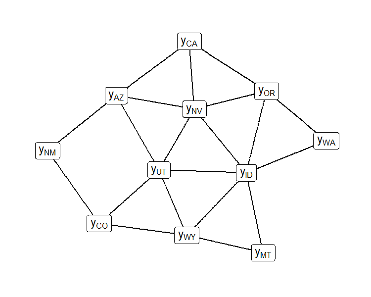
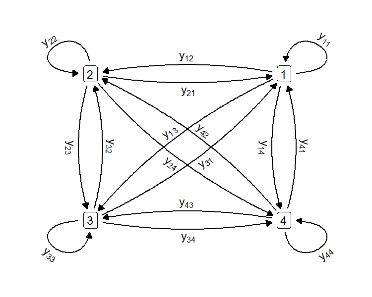
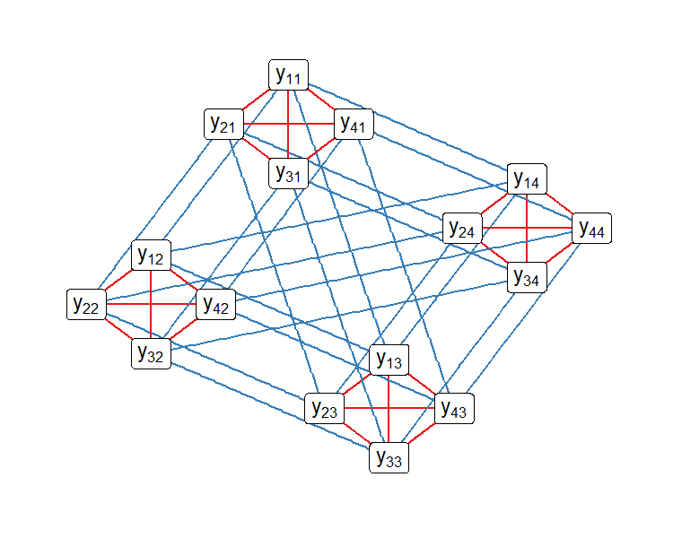
However, the dependence in network data is more complex than the dependence in spatial data. In the network setting, observations are made on the relationships between nodes, and shared nodes between two observations create dependence. This is in contrast to the areal spatial setting, where observations are made on discrete, disjoint areas and the neighbor relation between areas creates dependence (Figure 1, A & B). The additive random effects in (5), reflect two different ways in which network observations can be related: sharing a sender node (observations and ) and sharing a receiver node (observations and ). These two types of dependence result in a complex dependence structure (Figure 1, C & D). For each of these two types of dependence, the observations are divided into groups of observations which are all mutually dependent within a group.
Spatial models in which regions can be neighboring in two distinct ways have been studied in Reich et al., (2007) for the case of periodontal health measurements. Measurements were considered to be neighboring other measurements on the same tooth, or measurements on an adjacent tooth, but these kinds of neighbor relations were considered to create different kinds of dependence between measurements. The dependence in the periodontal health measurements was modeled using the random effect prior
| (12) |
where and are Laplacians for each neighbor relation. However, the distribution in (12) cannot represent the same dependence as the sender and receiver random effects in (5) because the distribution of is full rank, while the distribution of the vectorized is not full rank.
In this paper we introduce Restricted Network Regression as a method that mitigates network confounding. We approach network regression in a Bayesian framework, estimating parameters using their posterior distributions given the data. We characterize the posterior mean and variance of regression parameters in Restricted Network Regression with continuous data and show through simulation that Restricted Network Regression mitigates network confounding for continuous and binary data. Specifically, we demonstrate that a Restricted Network Regression model results in smaller bias and posterior credible intervals that are more appropriately calibrated to capture the generative parameter values than corresponding network regression models without random effects or with non-restricted random effects.
The remainder of this paper is organized as follows. Section 2 defines network confounding and requirements for methods to “alleviate” and “mitigate” network confounding. Section 3 introduces Restricted Network Regression, characterizes the collinearity of effects within the Restricted Network Regression model, and provides theorems about the posterior distribution of the regression parameters in the continuous Restricted Network Regression model. Section 4 describes the results of a simulation study involving both continuous and binary network regression. Section 5 is a case study of Eurovision Song Contest voting data showing the changes in inference that occur when using a Restricted Network Regression approach, relative to models without random effects and non-restricted random effect models. Finally, Section 6 closes with a discussion.
2 Network Confounding
Network confounding is the collinearity between fixed effects and network-structured random effects in a network regression model. This collinearity creates difficulty in estimating regression parameters by introducing bias in estimates and increasing their posterior variance. In this section we explore network confounding in more detail and define conditions for a method to alleviate or mitigate network confounding.
Consider the network regression model,
| (13) | ||||
| (14) | ||||
| (15) | ||||
| (16) | ||||
| (17) |
where is an -vector of latent continuous responses, is an fixed matrix of covariates, is a -vector of regression parameters, and and are -vectors composed of sender and receiver random effects, respectively, for each node in the network. The matrices and are matrices of zeros and ones which broadcast the elements of and into the appropriate rows of depending on the sender and receiver of each dyad. To match the vectorized form of , we write as an -vector of the observed network data.
Now consider partitioning into an intercept, an matrix of sender covariates , an matrix of receiver covariates , and an matrix of dyadic covariates as done in Hoff, (2021), where , , and are the number of sender, receiver, and dyadic covariates, respectively, and . Similarly, partition . The column space of the matrix contains all -vectors that have repeated values for dyads with a common sender. Similarly, the column space of the matrix contains all -vectors that have repeated values for dyads with a common receiver. Since the columns of are sender covariates, every column of is in the column space of . Therefore, we can write , where is an matrix created by collapsing equivalent rows of . Since the columns of are receiver covariates, every column of is in the column space of , allowing us to write . The model in (14) can be written
| (18) | ||||
| (19) |
From this, we can see that and are confounded in the sense that they occupy the same linear space in the response, i.e., , where is the column space operator. Similarly, and are also confounded. By restricting the random effects to be orthogonal to the fixed effects, Restricted Network Regression (introduced formally in the next section) fixes this collinearity by removing the intersection of the column spaces of , , and .
We now distinguish between two types of methods: those that alleviate network confounding and those that mitigate network confounding. We adapt a definition from the spatial statistics literature to define what it means for a method to alleviate network confounding:
Definition 1.
A network regression method modeling network data, , with unconditional regression parameters, , which results in posterior mean and marginal posterior variances alleviates network confounding if the following conditions are met:
-
1.
-
2.
for
Here are the unconditional regression coefficients of the corresponding network model without network-structured random effects and are the conditional regression coefficients from a model with non-restricted network-structured random effects.
Definition 1 is adapted from the definition of spatial confounding in Khan and Calder, (2022). This definition of alleviating network confounding reflects the intuition that models with network confounding will result in excess uncertainty on regression parameter estimates, reflected in large posterior variances of those parameters and that a method that alleviates network confounding should have lower posterior variances than one exhibiting network confounding. At the same time, a model that alleviates network confounding should model the unconditional effects of the fixed covariates, and so is expected to have the same posterior means as the model without network-structured random effects.
Alleviation of network confounding has useful interpretation in terms of parameter uncertainty, however, it does not relate directly to the accuracy of estimates made using models with network confounding. Also, Definition 1 provides no way to compare two models if neither alleviates network confounding. For these reasons, we introduce an alternative notion of network confounding mitigation. We expect a method that mitigates network confounding relative to another approach to produce better estimates and uncertainty quantification of the unconditional regression effects . We give a more precise definition of this mitigation:
Definition 2.
A network regression method modeling network data, , with unconditional regression parameters, , which results in posterior mean , denoted , and marginal posterior credible intervals , , for components , mitigates network confounding relative to another method which produces and , if for true unconditional regression effects ,
-
1.
for ,
-
2.
for ,
where the expectation in item 1 and probability in item 2 are taken over .
Definition 2 combines two useful model evaluations, bias and credible interval coverage, into a comparison which can be used to evaluate the relative improvement of one model over another in the presence of network confounding. Even if a model does not meet the requirements of Definition 1, it can be compared to other models using Definition 2 to assess its mitigation of network confounding.
3 Restricted Network Regression
For the network regression model given in (14) - (17), we propose the following Restricted Network Regression model:
| (20) | ||||
| (21) | ||||
| (22) | ||||
| (23) |
where , , , , , , and are as described earlier. This model is distinguished from the model in (14)-(17) by the application of the projection matrix projecting the random effects orthogonal to the column space of , and the interpretation of the regression effects, , as unconditional on the values of the random effects. With related to the unconditional regression parameters, by the regression equation (20) is equivalent to (14).
3.1 Properties of Continuous Restricted Network Regression Posterior Distributions
In this section, we provide relationships between the posterior means and variances of Restricted Network Regression and a model without random effects. With these relationships, we show that Restricted Network Regression with a continuous response does not satisfy the conditions of Definition 1, and therefore does not alleviate network confounding. We also relate these theoretical results to recent results in the spatial statistics literature by Khan and Calder, (2022), which showed a similar result in spatial regression.
To understand the behavior of the Restricted Network Regression model with respect to network confounding, we give an expression for the posterior mean and variance of in the Restricted Network Regression model.
Theorem 1.
In a continuous Restricted Network Regression model with two additive normally distributed node-level random effects,
| (24) | ||||
| (25) | ||||
| (26) |
the posterior distribution of will have mean and variance
| (27) | ||||
| (28) |
The proof of this theorem is provided in Appendix A of the Supplementary Material (Taylor et al.,, 2023). The prior distribution of is not specified for this theorem, but will partially determine . The posterior mean in (27) is equal to the posterior mean from a model without network-structured random effects, as required by Definition 1. Therefore Restricted Network Regression alleviates network confounding if and only if the inequality on the posterior variances in Definition 1 is true. We show this property of the posterior variances using a more general model with two restricted random effects.
Theorem 2.
Consider the restricted regression model with two random effects,
| (29) | ||||
| (30) | ||||
| (31) | ||||
| (32) | ||||
| (33) |
If and have orthonormal columns such that , and are pairwise orthogonal, and are positive definite symmetric matrices, for , and
| (34) |
where for , then for .
The proof of this theorem is provided in Appendix A of the Supplementary Material (Taylor et al.,, 2023). This theorem shows that under the specified conditions, a model with two random effects restricted to be orthogonal to the covariates yields posterior variances that do not meet the conditions in Definition 1. Applying Theorem 2 to Restricted Network Regression with , , and shows that Restricted Network Regression with a continuous response does not meet the conditions in Definition 1.
Khan and Calder, (2022) prove similar theorems for restricted spatial regression models of the form,
| (35) | ||||
| (36) | ||||
| (37) |
observing that that the model form in (35)-(37) encompasses the ICAR model, the non-spatial model, and restricted spatial regression models from Reich et al., (2006), Hughes and Haran, (2013), and Prates et al., (2019). The model in (35)-(37) is “restricted” if and are orthogonal. In fact, this form also encompasses continuous network models that include one additive sender or one additive receiver random effect, but not both, motivating the need for Theorem 2.
4 Simulation Study
In this section we investigate properties of Restricted Network Regression through simulations. We confirm the theoretical results from Section 3.1 using continuous network data and show that neither continuous nor binary Restricted Network Regression alleviate network confounding. However, we show that both mitigate network confounding relative to non-restricted network regression and network regression with no random effects. All of the following simulations involve data with varying levels of excess nodal variation, using models with both sender/receiver covariates and sender/receiver random effects.
In addition to evaluating Restricted Network Regression, we chose to evaluate choices of prior distribution on and . A common choice is the inverse-gamma distribution, e.g., in the amen package (Hoff et al.,, 2020). However, the half-Cauchy distribution, , is a less informative distribution recommended by Gelman, (2006) for random effect variances in hierarchical models. We compare five models:
-
(NoRE)
Network model with no random effects,
-
(NR.ig)
Network model with additive random effects and inverse-gamma priors,
-
(NR.hc)
Network model with additive random effects and half-Cauchy priors,
-
(RNR.ig)
Network model with restricted additive random effects and inverse-gamma priors,
-
(RNR.hc)
Network model with restricted additive random effects and half-Cauchy priors.
We show that Restricted Network Regression mitigates network confounding by providing estimates of with lower bias and properly calibrated credible intervals.
4.1 Simulation 1: Continuous Network Data
Continuous network data were simulated from the network model in (14)-(17), using the identity function, . The design matrix contained an intercept, one sender covariate, one receiver covariate, and one dyadic covariate whose values were drawn independently from a standard normal distribution. Unobserved excess nodal variation (simulated values of and , denoted and ) was then simulated from one of seven possible scenarios, which varied in the magnitude of the nodal variation and the degree of collinearity between the nodal variation and observed covariates. We control and quantify this latter degree of collinearity using the canonical correlation () between and .
-
(G1)
No excess variation: ,
-
(G2)
Small magnitude, no correlation:
, , , -
(G3)
Small magnitude, slight correlation:
, , , -
(G4)
Small magnitude, strong correlation:
, , , -
(G5)
Large magnitude, no correlation:
, , , -
(G6)
Large magnitude, slight correlation:
, , , -
(G7)
Large magnitude, strong correlation:
, , .
In all scenarios, the components of and were first generated i.i.d., then the vectors were projected to have the desired canonical correlation according to the algorithm in Appendix B of the Supplementary Material (Taylor et al.,, 2023). Scenarios G2, G3, and G4 were chosen to represent nodal variation smaller than the effect of one covariate, while scenarios G5, G6, and G7 were chosen to represent variation comparable to the effect of one covariate. The slight correlation scenarios (G3 and G6) represent situations with subjectively low correlation between nodal variation and covariates, while the strong correlation scenarios (G4 and G7) represent situations with subjectively high correlation between nodal variation and covariates. For each of the seven scenarios, 100 values of , , and were generated. Then for each set of covariates and random effects, 200 values of the random error were generated each from a standard normal distribution (), resulting in 20,000 simulated data sets for each scenario.
| (A) |
|
| (B) |
|
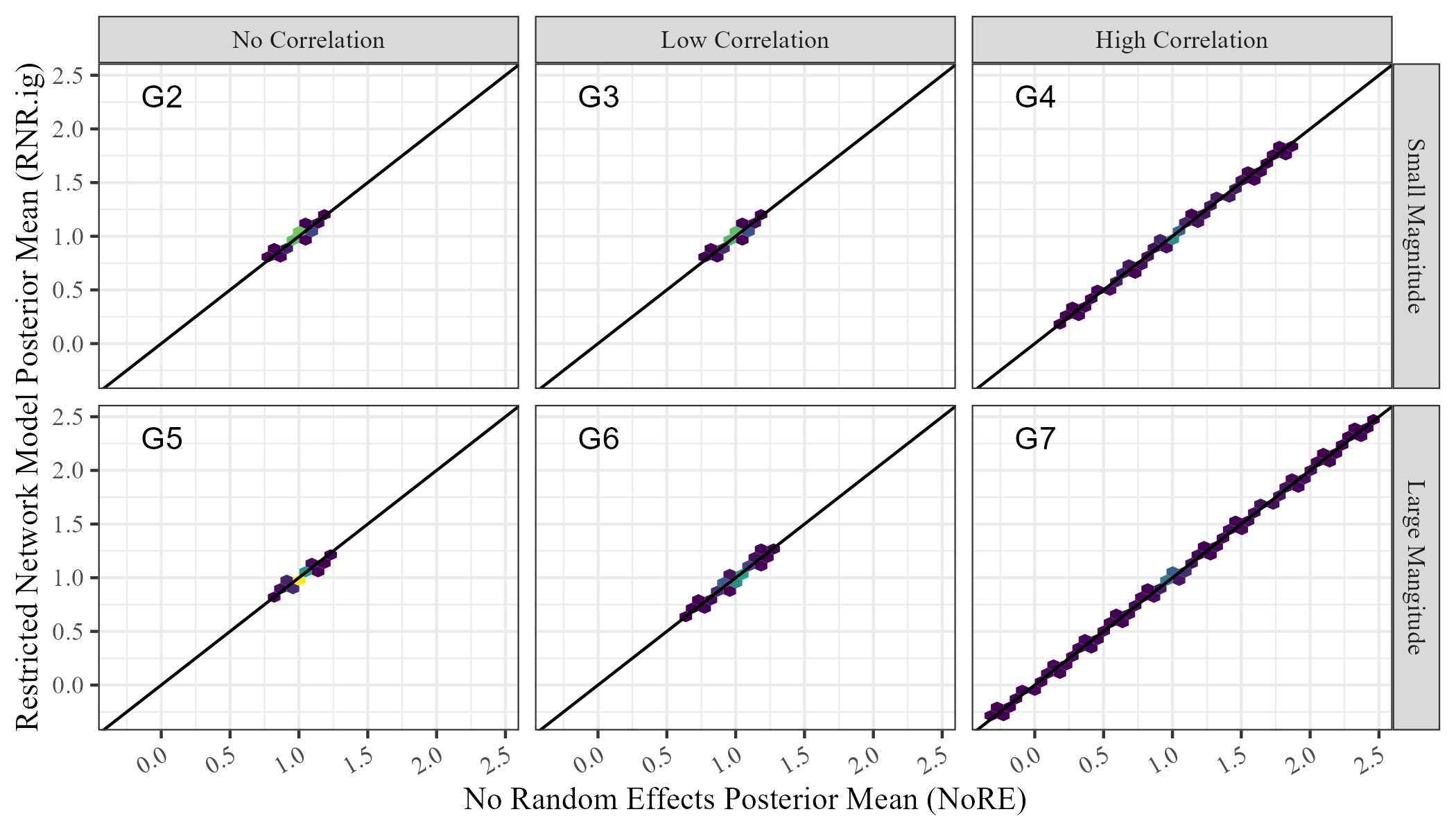
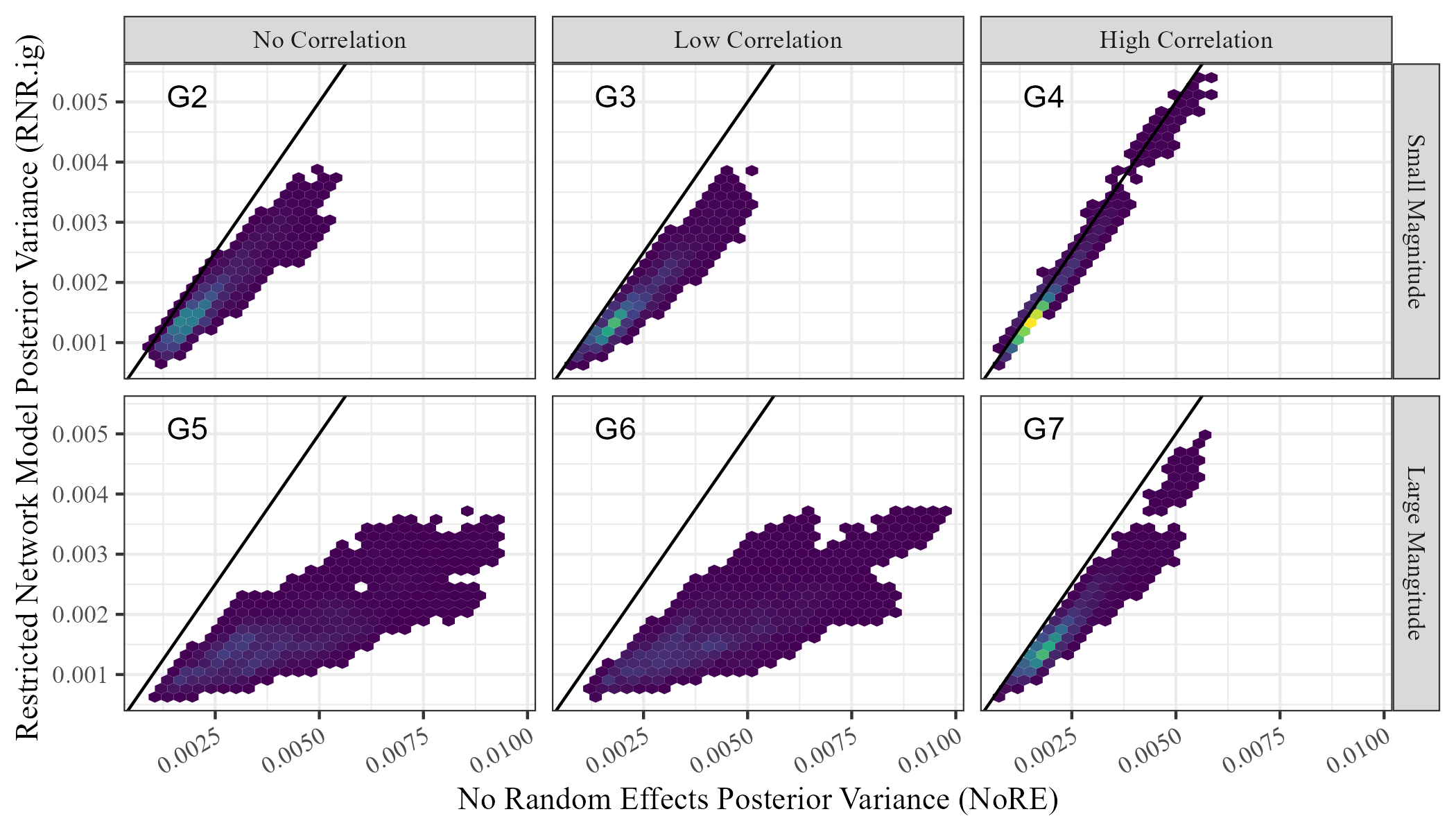
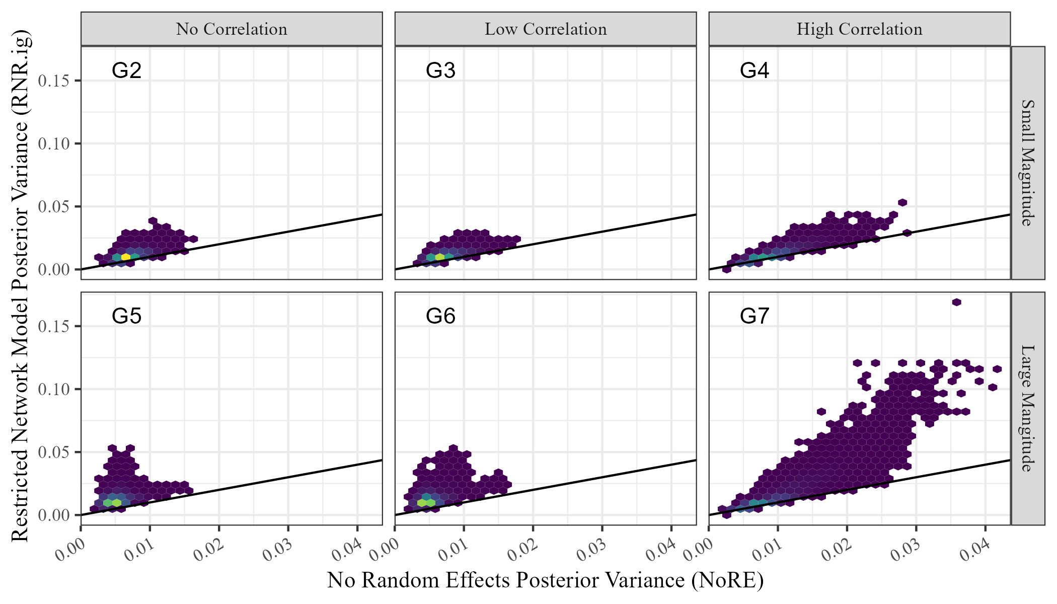
We compare the posterior means and posterior variances of the unconditional regression parameters in NoRE and RNR.ig. Figure 2 shows these values for the receiver covariate, . We see that the posterior means are equal for both models on all simulated data sets, and the posterior variance in the Restricted Network Regression model (RNR.ig) is less than or equal to the posterior variance in the model with no random effects (NoRE). Similar results were observed for the sender covariate. The equality of posterior means and this observed inequality of posterior variances validate the result of Theorem 2 empirically, and show that continuous Restricted Network Regression does not alleviate network confounding according to Definition 1.
| (A) |
|
| (B) |
|
To investigate the ability of Restricted Network Regression to mitigate network confounding relative to a model with no random effects and models with non-restricted random effects, we compare bias and coverage of posterior credible intervals for across all models (NoRE through RNR.hc). For each of the 200 trials with each of the 100 values of , , and , we recorded the difference between the posterior means of and and the value used to generate the data. We also recorded whether the 90% credible for captures . Finally we calculated the average bias across the 200 values of generated for each of the 100 values of , and the proportion of the 200 trials for which was captured by the credible interval.
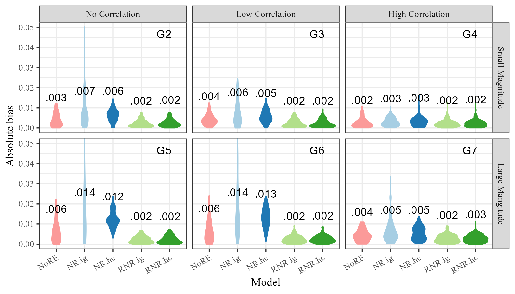
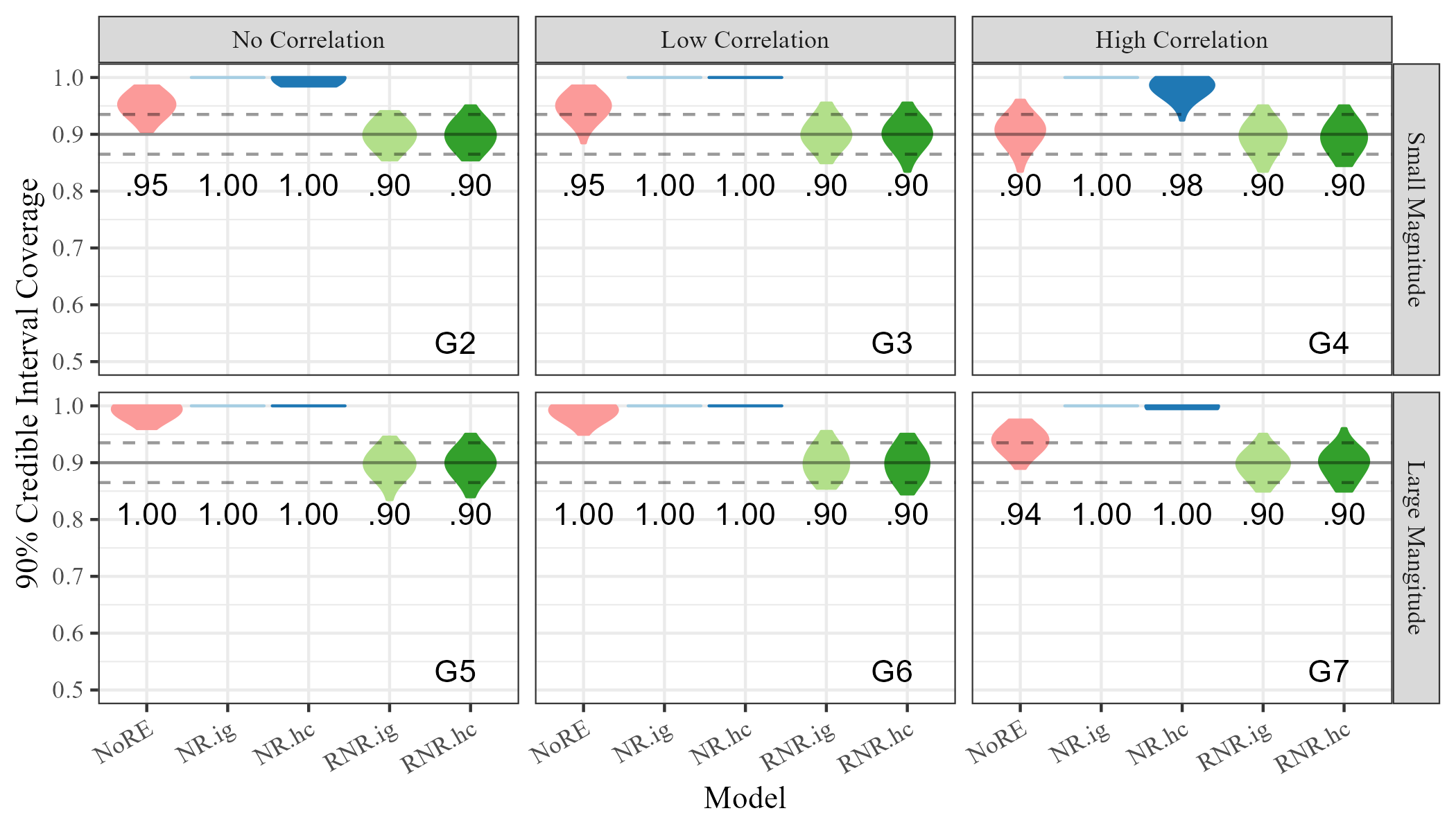
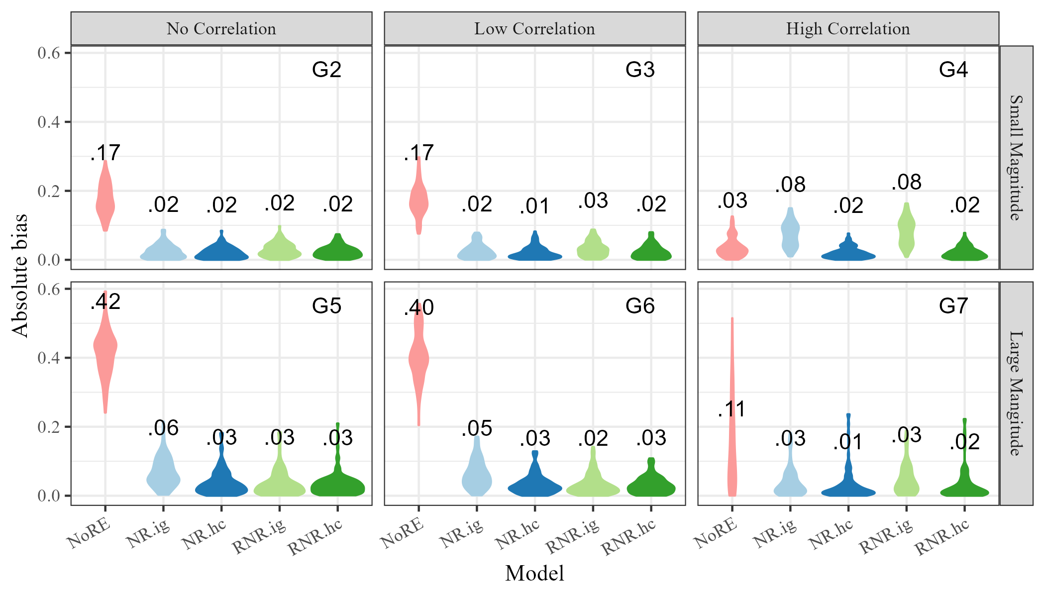
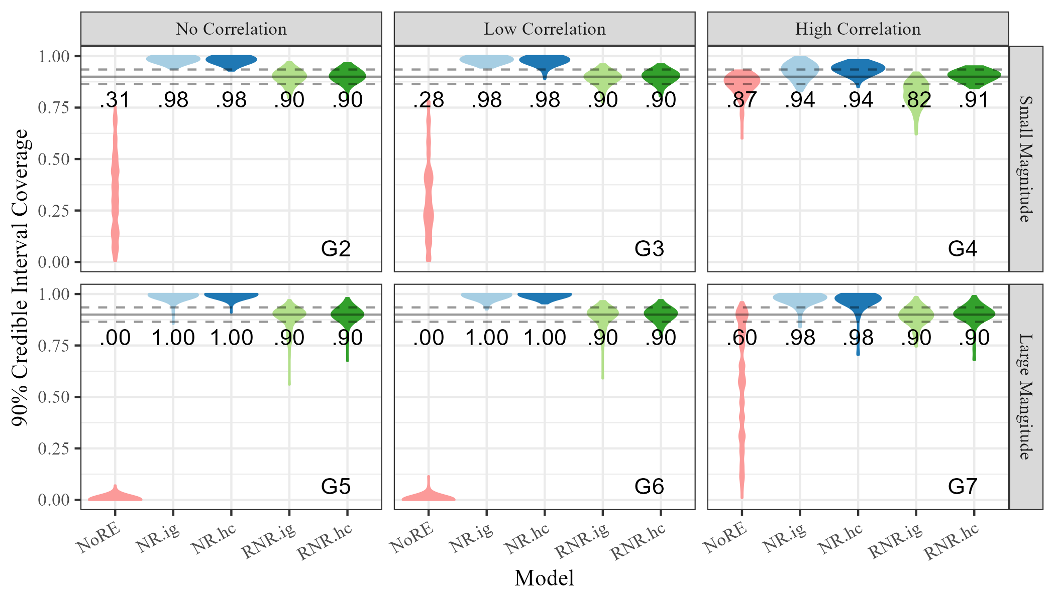
Figure 3 shows the distribution of the absolute bias and credible interval coverage for using each model in each scenario, G2 through G7. Bias appears lower for the restricted models (RNR.ig and RNR.hc) than for other models in scenarios G2, G3, G5, G6, and G7, and approximately equal in G4. The most noticeable difference between the Restricted Network Regression models and others is in credible interval coverage, where models RNR.ig and RNR.hc appear properly calibrated and NoRE, NR.ig, and NR.hc have coverage that is too high. Together, these results suggest the continuous Restricted Network Regression mitigates network confounding relative to both non-restricted network regression and network regression with no random effects.
4.2 Simulation 2: Binary Network Data
Data for the binary network models were simulated in the same way as for the continuous network model (Section 4.1), using scenarios G1 through G7, but with the indicator function to convert latent continuous responses to binary responses. All models were fit to each set of simulated data. We similarly assessed the results of these simulations by comparing posterior means and posterior variances of the unconditional regression parameters in models NoRE and RNR.ig.
| (A) |
|
| (B) |
|
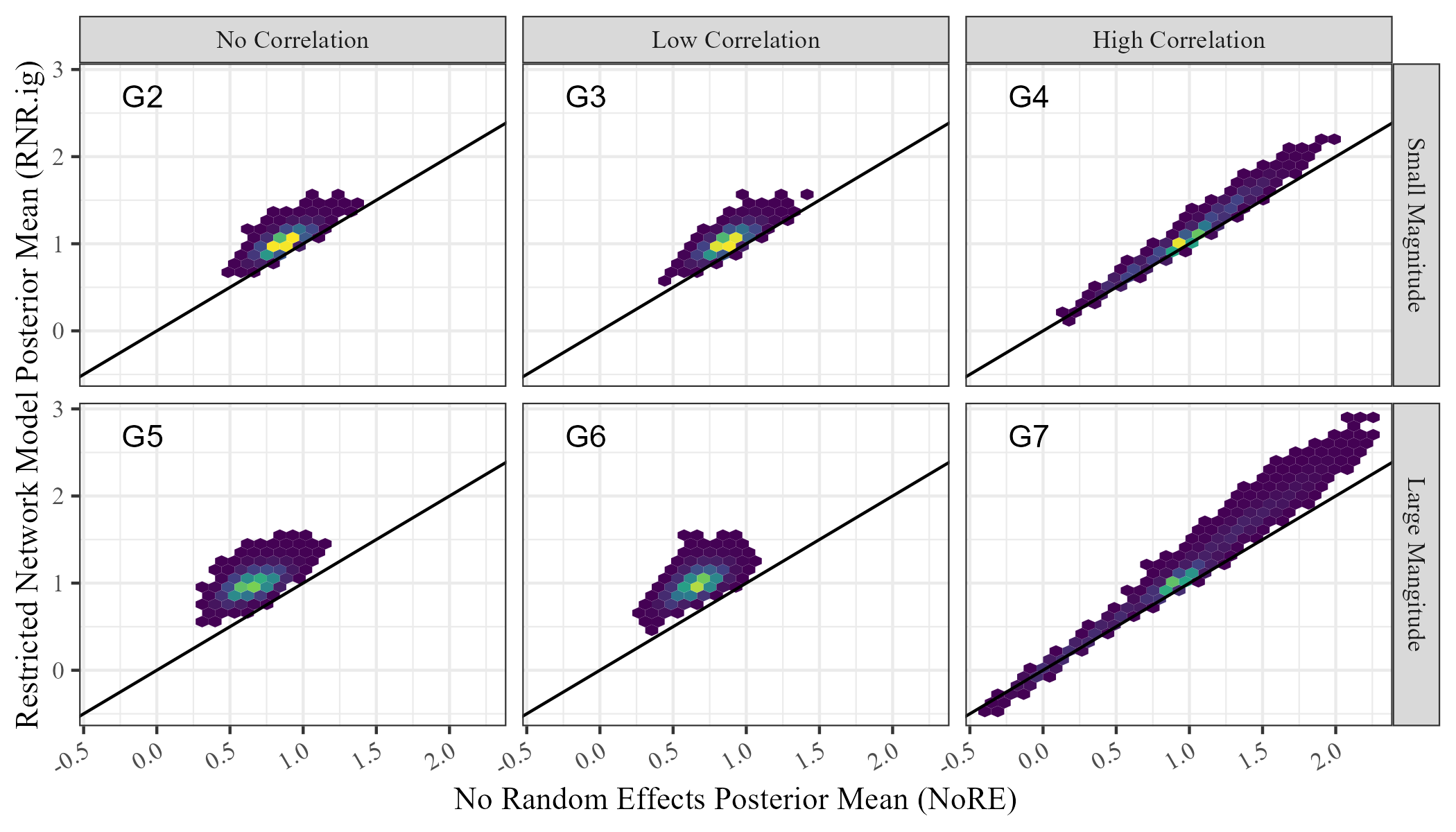
Figure 4 shows the comparison between posterior means and variances of for models NoRE and RNR.ig with binary data. This comparison is notably different from the comparison for continuous data in Figure 2. First, the posterior means produced by each model are not equal. Second, the posterior variance of the regression coefficient in the Restricted Network Regression model is now greater than in the network model with no random effects. This demonstrates empirically that the implications of Theorem 1 and Theorem 2 do not apply to models with non-Gaussian responses due to the inequality of posterior means. However, this inequality of means also demonstrates that probit Restricted Network Regression also does not alleviate network confounding.
| (A) |
|
| (B) |
|
Figure 5 shows the absolute bias and coverage estimates for in scenarios G2 through G7 using all models. The bias for model NoRE is the highest in general, with all other models having approximately equal absolute bias except in scenario G4. In most scenarios, the coverage of model NoRE is significantly lower than 90%, while the coverage of the Restricted Network Regression model with both inverse-gamma (RNR.ig) and half-Cauchy (RNR.hc) priors is much closer to 90%. Again, the non-restricted models (NR.ig and NR.hc) have coverage that is higher than 90% in all scenarios. The Restricted Network Regression model with half-Cauchy random effect priors (RNR.hc) has coverage within the expected range in all scenarios. A notable exception is scenario G4, in which the models with inverse-gamma priors on and (NR.ig and RNR.ig), have higher bias than their half-Cauchy counterparts. The coverage for model RNR.ig is also noticeably lower than RNR.hc. Here, the prior selection affects the model’s ability to mitigate network confounding. While model RNR.hc mitigates network confounding relative to NR.hc and RNR.ig mitigates network confounding relative to NR.ig, RNR.ig does not mitigate network confounding relative to NR.hc due to higher bias in this scenario.
5 Eurovision Voting Network Analysis
The Eurovision Song Contest is an annual competition in which European countries compete by submitting the best song by an artist from their country. The contest culminates in a final round, where the remaining 26 competitors perform their songs for a TV audience. All participating countries then vote for their top ten songs through judges and/or phone-in voting. Points are awarded according to votes (12 points for first, 10 points for second, then 8 through 1 points for third through tenth) and the total determines the winner.
The contest is extremely popular, drawing 182 million viewers in 2019 (Eurovision,, 2019). This popularity has meant that the contest has been of interest for study, especially the study of voting patterns (e.g., Ginsburgh and Noury,, 2008; Spierdijk and Vellekoop,, 2009). Because competing countries are a subset of voting countries, vote data can naturally be represented as a directed graph with the countries as nodes and an edge from country to country representing a top-10 vote by country for country . Edges may be labeled with ranked votes if desired. Eurovision votes have been analyzed as a network by, for example, Yair, (1995), Fenn et al., (2006), and D’Angelo et al., (2019).
Countries may have other measurable qualities that are related to how well they score in the contest results. For example, countries with larger populations have more musicians from which to select a contestant. A country’s wealth may be associated with the reach of its cultural exports, leading to more votes received from its trading partners. The Eurovision Song Contest is also the subject of bets predicting its winner. Betting markets reflect the collective knowledge of their participants, which in this case includes knowledge of the specific songs entered by each country, and it is reasonable to think they may be predictive of the outcome. For example, Spann and Skiera, (2009) finds betting odds to be predictive of match results in the German premier soccer league. Analyzing the relationship between population, wealth, and betting odds, and the Eurovision contest voting outcome fits a network regression framework naturally.
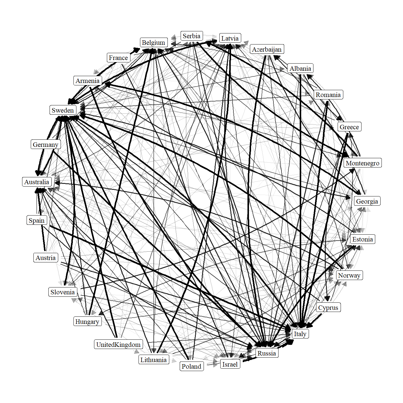
We restrict our analysis to the year 2015 and the 27 countries with entries in the final round of that year (Australia, as a new contestant, was given an automatic berth to the final round). The response data consist of a vote network represented as a matrix (Figure 6). The receiver covariate data consist of three dimension 27 vectors of song or country attributes: the log median odds from 16 popular European betting sites for each song to win the contest, the log 2015 population of each competing country, and the log 2015 GDP per capita of each competing country. We log-transform the receiver covariates before using them as covariates in a regression model because they are either right-skewed (GDP, population) or because we believe there to be a logarithmic relationship between the predictor and the response (betting odds). We also include a dyadic covariate for country contiguity which was found to be explanatory in D’Angelo et al., (2019). Country contiguity is an undirected network represented as a symmetric binary matrix where a 1 indicates that two countries share a border and a 0 indicates otherwise. Visualizations of these covariates are available in Appendix C of the Supplementary Material (Taylor et al.,, 2023). Votes were represented as ranks (1-10 with 10 the highest). This data is freely available and easily compiled by hand (Eurovision,, 2015; Eurovisionworld,, 2015; Conte et al.,, 2022; United Nations,, 2015; World Bank,, 2022). Any pairs where country did not vote for country in its top 10 were coded as zero. Our focus on a single year is due to the fact that both betting odds and column random effects are song-specific, and therefore year-specific. Therefore additional years in this analysis cannot be treated like replicates in the style of D’Angelo et al., (2019). We examine the effects of the covariates on Eurovision voting by performing a network regression analysis without random effects, with receiver random effects, and with restricted receiver random effects. We investigate the effect of Restricted Network Regression on regression parameter estimates and interpretation compared to either alternative model.
5.1 Network Model with No Random Effects
The base model with no network-structured random effects has the form,
| (38) | ||||
| (39) | ||||
| (40) |
We used the relative rank likelihood (RRL; Pettitt,, 1982; Hoff et al.,, 2013), implemented with a function which maps continuous values to the observed ranks in the following way: for any voting country and two entered songs and , implies . This imposes no relationship between the responses for different voting countries, so we cannot infer row effects (Hoff et al.,, 2013).
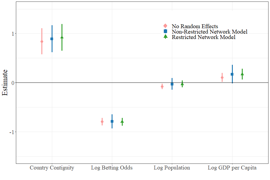
We analyze and interpret the regression parameter estimates through posterior means and 90% credible intervals for (Figure 7). As these are estimates of and there are no random effects in the model, we interpret them as the unconditional effect of the fixed effects on the response. All fixed covariates–country contiguity, log betting odds, log GDP per capita, and log population–appear to have an effect on the voting outcomes. Country contiguity has a large positive effect, agreeing with D’Angelo et al., (2019) that countries are more likely to vote for their neighbors’ songs. Log betting odds have a large negative effect, which shows that betting markets are predictive of the Eurovision outcome as larger odds are associated with lower predicted probability of winning. Log GDP per capita has a small positive effect, indicating that wealthier countries are more likely to receive votes than less wealthy countries. Log population has a small negative effect. All other things being equal, more populous countries are less likely to receive votes than less populous countries.
5.2 Non-Restricted Network Model
We fit a network model with a receiver random effect () to account for song heterogeneity not explained by the betting odds, population, or GDP. This network model has the form,
| (41) | ||||
| (42) | ||||
| (43) | ||||
| (44) |
Leaving the random effects non-restricted is appropriate depending on the intended interpretation of the terms in the model. For example, restricted regression is not recommended in the case of “Scheffé-style” random effects: random effects whose values are considered as draws from a population which is of interest, even though the values of the effects themselves are not (Hodges and Reich,, 2010). If we consider the population of countries to be all those eligible to participate in the contest, or all those who competed in the initial rounds, then the selection of countries in the final round is only a subset of the population. If the primary interest is studying the population of all eligible countries rather than the propensity of individual countries to receive votes, the receiver random effects could be considered “Scheffé-style” and restricted regression may not be an appropriate choice.
Because the model contains receiver random effects, the regression effects represent the effect of the covariates on the response conditioned on . The posterior means and credible intervals of the regression parameters in this model are noticeably different than in the network model without random effects (Figure 7). In this case, the country contiguity retains its large positive effect and log betting odds retains its large negative effect. We notice that the width of the 90% posterior credible intervals for , , and are wider than the credible intervals for , , and from the model in (39), indicating greater uncertainty about the conditional effect of these covariates than the unconditional effect. The estimate of is also smaller in magnitude and has a credible interval which includes zero. The changes in credible interval width and posterior mean illustrate the impact of network confounding.
| Comparison Model | ||||
|---|---|---|---|---|
| No Random Effects | Non-Restricted Model | |||
| Covariate | Mean Ratio | Width Ratio | Mean Ratio | Width Ratio |
| Log Betting Odds | 1.004 | 1.045 | 1.008 | 0.539 |
| Log Population | 0.389 | 1.247 | 1.000 | 0.598 |
| Log GDP per Capita | 1.656 | 1.173 | 1.004 | 0.566 |
| Country Contiguity | 1.091 | 1.031 | 1.032 | 0.997 |
5.3 Restricted Network Model
We fit a network model with a receiver random effect () to account for song heterogeneity not explained by the column covariates, projected to be orthogonal to the fixed effects of betting odds, population, or GDP. Specifically, we set
| (45) | ||||
| (46) |
Since the association between and is of primary interest, we would like estimates of instead of . If we do not want to infer about the population of countries which did not compete in this year’s final round, then the random effects in the model constitute the entire population of interest. Since in this analysis we are using data only from the final round of the 2015 contest, restricted regression would be appropriate. In the Restricted Network Regression model, the regression effects once again represent the unconditional effect of the covariates on the response as the collinearity with the random effect has been removed.
Table 1 compares the magnitude of the regression parameter estimates and their credible interval widths from the Restricted Network Regression model to those in the other models. Compared to the model with no random effects, the receiver effects for log population and log GDP per capita exhibit noticeably different posterior means and larger posterior credible intervals, while the effect for log betting odds shows approximately equal posterior mean and only slightly larger credible interval (Figure 7). These results mirror what was observed with the binary data in the earlier simulation study. Based on that study, we expect the estimates from Restricted Network Regression to more accurately capture the unconditional effect of the covariates on the response. Compared to the non-restricted network model, all regression parameters have approximately equal posterior means and the receiver covariate effects have smaller posterior credible intervals. Restricted Network Regression allows the excess network-structured variation in to be accounted for via the random effects , while avoiding the network confounding and inflated standard errors in the non-restricted network model.
6 Discussion
In this paper, we introduced Restricted Network Regression for models with additive network random effects and established its connection to restricted spatial regression. We characterized the network confounding of the network regression model with additive random effects and node-level covariates, which Restricted Network Regression addresses by forcing the column spaces of the fixed and random effects to be mutually orthogonal. We provided conditions for network regression models to alleviate and mitigate network confounding, and proved that Restricted Network Regression does not alleviate network confounding with theoretical results and through simulation. However, we showed through simulation that Restricted Network Regression does mitigate network confounding relative to network regression with no random effects and non-restricted network regression with continuous and binary response data. Restricted Network Regression produces less bias and properly calibrated credible intervals for regression parameters relative to network regression without random effects and non-restricted network regression.
We also explored through simulation the effect of a half-Cauchy prior on the variance components of the network random effects. We found that this prior resulted in comparable bias and credible interval coverage for the unconditional regression effects to the conjugate inverse-gamma prior in probit Restricted Network Regression, with better bias and credible interval coverage in some scenarios.
Finally, we applied Restricted Network Regression to a dataset of Eurovision Song Contest voting. We interpreted the model estimates of Restricted Network Regression alongside those from a model without network-structured random effects and those from a non-restricted network regression model. For the three receiver covariates in the model, the choice of model affected both their posterior mean point estimates and their credible interval estimates. The change in credible interval width is noticeable for all three receiver covariates. Uncertainty, as indicated by the width of posterior credible intervals, increases after adding random effects to the model, but decreases again after restricting them. The widths of the credible intervals for the receiver covariates with restricted random effects is larger than without random effects but smaller than with non-restricted random effects.
Future work in this area includes developing Restricted Network Regression for other forms of network random effects such as multiplicative effects (Hoff,, 2021) or latent space distance effects (Hoff et al.,, 2002). It is less clear which covariates may be confounded with such effects, and whether restricting these random effects can have the same benefits as with additive effects and non-Gaussian data. Theoretical results for binary or other non-Gaussian data that describe the posterior distribution are also needed to make stronger conclusions about Restricted Network Regression on non-Gaussian data. Restricted network regression can also be expanded to include bipartite network data or longitudinal network data (e.g., Marrs et al.,, 2020).
Supplement
Supplement to “Restricted Regression in Networks”
This supplementary document contains proofs of theorems in this paper, additional theorems not presented in this paper, details of simulation studies and details of data analysis.
Acknowledgements
K. Keller acknowledges the support of NSF Grant 1856229 for this work.
References
- Albert and Chib, (1993) Albert, J. H. and Chib, S. (1993). Bayesian analysis of binary and polychotomous response data. Journal of the American Statistical Association, 88(422):669–679.
- Aleskerov et al., (2017) Aleskerov, F., Meshcheryakova, N., Rezyapova, A., and Shvydun, S. (2017). Network analysis of international migration. In Kalyagin, V. A., Nikolaev, A. I., Pardalos, P. M., and Prokopyev, O. A., editors, Models, Algorithms, and Technologies for Network Analysis, pages 177–185, Cham. Springer International Publishing.
- Becker et al., (1995) Becker, R., Eick, S., and Wilks, A. (1995). Visualizing network data. IEEE Transactions on Visualization and Computer Graphics, 1(1):16–28.
- Besag et al., (1991) Besag, J., York, J., and Mollié, A. (1991). Bayesian image restoration, with two applications in spatial statistics. Annals of the Institute of Statistical Mathematics, 43(1):1–20.
- Campbell et al., (2019) Campbell, B. W., Marrs, F. W., Böhmelt, T., Fosdick, B. K., and Cranmer, S. J. (2019). Latent Influence Networks in Global Environmental Politics. PLOS ONE, 14(3):1–17.
- Cantner and Graf, (2006) Cantner, U. and Graf, H. (2006). The Network of Innovators in Jena: An Application of Social Network Analysis. Research Policy, 35(4):463–480.
- Clayton et al., (1993) Clayton, D. G., Bernardinelli, L., and Montomoli, C. (1993). Spatial Correlation in Ecological Analysis. International Journal of Epidemiology, 22(6):1193–1202.
- Conte et al., (2022) Conte, M., Cotterlaz, P., and Mayer, T. (2022). The CEPII Gravity Database. Working Papers 2022-05, CEPII.
- D’Angelo et al., (2019) D’Angelo, S., Murphy, T. B., and Alfò, M. (2019). Latent space modelling of multidimensional networks with application to the exchange of votes in Eurovision Song Contest. The Annals of Applied Statistics, 13(2):900 – 930.
- Eurovision, (2015) Eurovision (2015). Eurovision Song Contest 2015 Grand Final. https://web.archive.org/web/20150924042946/http://www.eurovision.tv/page/history/by-year/contest?event=2083#Scoreboard. Accessed 2023-09-15 via Internet Archive.
- Eurovision, (2019) Eurovision (2019). 182 million viewers tuned in to the 2019 Eurovision Song Contest. https://eurovision.tv/story/182-million-viewers-2019-eurovision-song-contest. Accessed 2023-09-14.
- Eurovisionworld, (2015) Eurovisionworld (2015). Odds Eurovision Song Contest 2015. https://eurovisionworld.com/odds/eurovision-2015. Accessed 2023-09-15.
- Fenn et al., (2006) Fenn, D., Suleman, O., Efstathiou, J., and Johnson, N. F. (2006). How does Europe Make Its Mind Up? Connections, cliques, and compatibility between countries in the Eurovision Song Contest. Physica A: Statistical Mechanics and its Applications, 360(2):576–598.
- Gelman, (2006) Gelman, A. (2006). Prior distributions for variance parameters in hierarchical models (comment on article by Browne and Draper). Bayesian Analysis, 1(3):515 – 534.
- Ginsburgh and Noury, (2008) Ginsburgh, V. and Noury, A. G. (2008). The Eurovision Song Contest. Is Voting Political or Cultural? European Journal of Political Economy, 24(1):41–52.
- Gwon et al., (2020) Gwon, Y., Mo, M., Chen, M.-H., Chi, Z., Li, J., Xia, A. H., and Ibrahim, J. G. (2020). Network Meta-Regression for Ordinal Outcomes: Applications in Comparing Crohn’s Disease Treatments, journal = Statistics in Medicine. 39(13):1846–1870.
- Hanks et al., (2015) Hanks, E. M., Schliep, E. M., Hooten, M. B., and Hoeting, J. A. (2015). Restricted spatial regression in practice: geostatistical models, confounding, and robustness under model misspecification. Environmetrics, 26(4):243–254.
- Hodges and Reich, (2010) Hodges, J. S. and Reich, B. J. (2010). Adding Spatially-Correlated Errors Can Mess Up the Fixed Effect You Love. The American Statistician, 64(4):325–334.
- Hoff, (2021) Hoff, P. (2021). Additive and Multiplicative Effects Network Models. Statistical Science, 36(1):34 – 50.
- Hoff et al., (2020) Hoff, P., Fosdick, B., and Volfovsky, A. (2020). amen: Additive and Multiplicative Effects Models for Networks and Relational Data. R package version 1.4.4.
- Hoff et al., (2013) Hoff, P., Fosdick, B., Volfovsky, A., and Stovel, K. (2013). Likelihoods for fixed rank nomination networks. Network Science, 1(3):253–277.
- Hoff, (2005) Hoff, P. D. (2005). Bilinear mixed-effects models for dyadic data. Journal of the American Statistical Association, 100(469):286–295.
- Hoff et al., (2002) Hoff, P. D., Raftery, A. E., and Handcock, M. S. (2002). Latent Space Approaches to Social Network Analysis. Journal of the American Statistical Association, 97(460):1090–1098.
- Holland et al., (1983) Holland, P. W., Laskey, K. B., and Leinhardt, S. (1983). Stochastic Blockmodels: First Steps. Social Networks, 5(2):109–137.
- Hughes and Haran, (2013) Hughes, J. and Haran, M. (2013). Dimension Reduction and Alleviation of Confounding for Spatial Generalized Linear Mixed Models. Journal of the Royal Statistical Society. Series B (Statistical Methodology), 75(1):139–159.
- Khan and Calder, (2022) Khan, K. and Calder, C. A. (2022). Restricted Spatial Regression Methods: Implications for Inference. Journal of the American Statistical Association, 117(537):482–494.
- Lee and Sohn, (2022) Lee, J. W. and Sohn, S. Y. (2022). Evaluating borrowers’ default risk with a spatial probit model reflecting the distance in their relational network. PLOS ONE, 16(12):1–11.
- Li et al., (2018) Li, H., Chen, M.-H., Ibrahim, J. G., Kim, S., Shah, A. K., Lin, J., and Tershakovec, A. M. (2018). Bayesian Inference for Network Meta-Regression Using Multivariate Random Effects With Applications to Cholesterol Lowering Drugs. Biostatistics, 20(3):499–516.
- Li and Loken, (2002) Li, H. and Loken, E. (2002). A unified theory of statistical analysis and inference for variance component models for dyadic data. Statistica Sinica, 12(2):519–535.
- Marrs et al., (2020) Marrs, F. W., Campbell, B. W., Fosdick, B. K., Cranmer, S. J., and Böhmelt, T. (2020). Inferring Influence Networks from Longitudinal Bipartite Relational Data. Journal of Computational and Graphical Statistics, 29(3):419–431.
- Marrs et al., (2022) Marrs, F. W., Fosdick, B. K., and Mccormick, T. H. (2022). Regression of exchangeable relational arrays. Biometrika, 110(1):265–272.
- Pettitt, (1982) Pettitt, A. N. (1982). Inference for the Linear Model Using a Likelihood Based on Ranks. Journal of the Royal Statistical Society. Series B (Methodological), 44(2):234–243.
- Prates et al., (2019) Prates, M. O., Assunção, R. M., and Rodrigues, E. C. (2019). Alleviating Spatial Confounding for Areal Data Problems by Displacing the Geographical Centroids. Bayesian Analysis, 14(2):623 – 647.
- Reich et al., (2007) Reich, B. J., Hodges, J. S., and Carlin, B. P. (2007). Spatial Analyses of Periodontal Data Using Conditionally Autoregressive Priors Having Two Classes of Neighbor Relations. Journal of the American Statistical Association, 102(477):44–55.
- Reich et al., (2006) Reich, B. J., Hodges, J. S., and Zadnik, V. (2006). Effects of Residual Smoothing on the Posterior of the Fixed Effects in Disease-Mapping Models. Biometrics, 62(4):1197–1206.
- Robins et al., (2007) Robins, G., Pattison, P., Kalish, Y., and Lusher, D. (2007). An Introduction to Exponential Random Graph (p*) Models for Social Networks. Social Networks, 29(2):173–191. Special Section: Advances in Exponential Random Graph (p*) Models.
- Sengupta and Chen, (2018) Sengupta, S. and Chen, Y. (2018). A Block Model for Node Popularity in Networks With Community Structure. Journal of the Royal Statistical Society: Series B (Statistical Methodology), 80(2):365–386.
- Spann and Skiera, (2009) Spann, M. and Skiera, B. (2009). Sports forecasting: A comparison of the forecast accuracy of prediction markets, betting odds and tipsters. Journal of Forecasting, 28(1):55–72.
- Spierdijk and Vellekoop, (2009) Spierdijk, L. and Vellekoop, M. (2009). The Structure of Bias in Peer Voting Systems: Lessons from the Eurovision Song Contest. Empirical Economics, 36(2):403–425.
- Taylor et al., (2023) Taylor, I., Keller, K. P., and Fosdick, B. K. (2023). Supplement to ‘Restricted Regression in Networks’.
- United Nations, (2015) United Nations (2015). The World Population Prospects: 2015 Revision. https://www.un.org/en/development/desa/publications/world-population-prospects-2015-revision.html.
- Wang and Wong, (1987) Wang, Y. J. and Wong, G. Y. (1987). Stochastic Blockmodels for Directed Graphs. Journal of the American Statistical Association, 82(397):8–19.
- Warner et al., (1979) Warner, R. M., Kenny, D. A., and Stoto, M. (1979). A New Round Robin Analysis of Variance for Social Interaction Data. Journal of Personality and Social Psychology, 37(10):1742–1757.
- World Bank, (2022) World Bank (2022). GDP per capita (constant 2015 US$). https://data.worldbank.org/indicator/NY.GDP.PCAP.KD. Accessed 2023-09-15.
- Yair, (1995) Yair, G. (1995). ‘Unite Unite Europe’ The Political and Cultural Structures of Europe as Reflected in the Eurovision Song Contest. Social Networks, 17(2):147–161.
- Zimmerman and Hoef, (2022) Zimmerman, D. L. and Hoef, J. M. V. (2022). On deconfounding spatial confounding in linear models. The American Statistician, 76(2):159–167.