Rethinking Latent Representations in Behavior Cloning: An Information Bottleneck Approach for Robot Manipulation
Abstract
Behavior Cloning (BC) is a widely adopted visual imitation learning method in robot manipulation. Current BC approaches often enhance generalization by leveraging large datasets and incorporating additional visual and textual modalities to capture more diverse information. However, these methods overlook whether the learned representations contain redundant information and lack a solid theoretical foundation to guide the learning process. To address these limitations, we adopt an information-theoretic perspective and introduce mutual information to quantify and mitigate redundancy in latent representations. Building on this, we incorporate the Information Bottleneck (IB) principle into BC, which extends the idea of reducing redundancy by providing a structured framework for compressing irrelevant information while preserving task-relevant features. This work presents the first comprehensive study on redundancy in latent representations across various methods, backbones, and experimental settings, while extending the generalizability of the IB to BC. Extensive experiments and analyses on the CortexBench and LIBERO benchmarks demonstrate significant performance improvements with IB, underscoring the importance of reducing input data redundancy and highlighting its practical value for more practical applications. Project Page: BC-IB Website.
1 Introduction
Behavior Cloning (BC), one of the simplest and most widely used methods in Imitation Learning (IL), learns a mapping from states to actions by training on state-action pairs from expert demonstrations. BC has been widely studied in autonomous driving (Bain & Sammut, 1995; Torabi et al., 2018), robotics control (Argall et al., 2009) and game AI (Pearce & Zhu, 2022). In robot manipulation, BC has become a foundational approach, enabling robots to replicate expert actions based on sensory inputs such as images or proprioception information like gripper states. To enhance the generalization of robots, most BC methods focus on incorporating large datasets of human or manipulation videos (Jang et al., 2022; Karamcheti et al., 2023; Brohan et al., 2023; Cheang et al., 2024; Saxena et al., 2025), or integrating additional text and visual information (Jia et al., 2024; Wen et al., 2024; Hu et al., 2024). While these methods have made significant progress in improving generalization by leveraging more diverse information, they often neglect a critical aspect: whether the learned representations contain significant redundant information.
Why do we need to explore this? Firstly, the inherent challenges of input data redundancy remain largely unexplored in BC for robot manipulation, despite their potential to significantly impact performance. Secondly, most existing methods lack a solid theoretical foundation to guide the learning process. Then, a key question arises: how can we quantify the redundancy in inputs or representations, and how can we effectively reduce it?
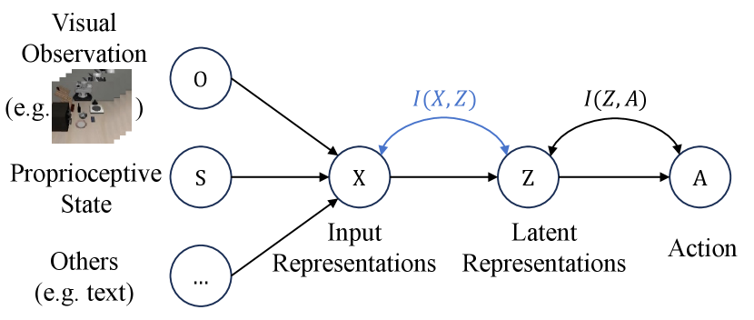
How to explore this? As illustrated in Figure 1, in BC, the inputs are typically encoded into individual representations and concatenated to form the input representation . This is then processed through a feature fusion module to produce the latent representation , which is subsequently decoded to predict the action . The policy is optimized by minimizing the discrepancy between the predicted actions and the expert-provided actions. In information theory, mutual information between and , denoted as , measures the amount of information gained about one random variable by knowing the other. In BC, if output can be well predicted by , reducing means continuously eliminating redundant information from .
Taking a step further, an information-theoretic approach that balances the trade-off between representation complexity and predictive power offers a natural framework to address the problem of latent representation redundancy and the lack of a solid theoretical foundation, namely information bottleneck (IB) principle (Tishby et al., 1999). IB regularizes the representation by minimizing the mutual information between and , while maximizing the mutual information between and . The first term represents the compression of the representation, where a smaller mutual information indicates a greater degree of compression and redundancy reduction, while ensures predictive power is maintained.
Motivated by this information-theoretic approach, we make the first attempt in this work to study the impact of latent representation redundancy in BC for robot manipulation and extend the IB method to this context, where redundancy in latent representations is quantified by . We conduct extensive experiments in various settings and analyses to validate its effectiveness, highlighting the benefits of reducing redundancy to enhance generalization in robotic tasks. Additionally, we provide detailed theoretical analyses, including generalization error bounds, to validate its effectiveness.
How to apply IB to the BC architectures, and what are its potential applications? To ensure the generality of our findings, we categorize BC architectures based on their feature fusion methods into two types: spatial fusion and temporal fusion. This allows us to identify the applicable scenarios for each fusion method, and by incorporating IB, we uncover a series of interesting findings. Furthermore, our experiments reveal that regardless of the pre-training stage, the final fine-tuning phase, or the size of the dataset, incorporating IB by reducing redundancy enables the model to learn more robust features and improve performance, suggesting its potential applicability in these scenarios.
Our contributions are three-fold. (1) We extend the IB to BC and provide a comprehensive study on the impact of latent representation redundancy in BC for robot manipulation. (2) We empirically demonstrate that minimizing redundancy in latent representations helps existing BC algorithms significantly improve generalization performance on the Cortexbench and LIBERO benchmarks across various settings, indirectly highlighting the considerable redundancy present in current robot trajectory datasets. (3) We provide a detailed theoretical analysis explaining why IB enhances the transferability of BC methods.
2 Related Work
2.1 Behavior Cloning in Robot Manipulation
Behavioral Cloning (BC), first introduced by (Pomerleau, 1991), is a well-known Imitation Learning (IL) algorithm that learns a policy by directly minimizing the discrepancy between the agent’s actions and those of the expert in the demonstration data. To learn more generalizable representations, one class of visual representation learning methods pre-train on large video datasets of robotics or humans, enabling rapid application of the pre-trained encoder to downstream robotic tasks. Notable examples include VC-1 (Majumdar et al., 2023), R3M (Nair et al., 2023), and Voltron (Karamcheti et al., 2023) . Meanwhile, another line of research focuses on training on even more extensive and diverse datasets with larger models, such as Internet-scale visual question answering and robot trajectory data (Brohan et al., 2023), as well as a vast collection of Internet videos (Cheang et al., 2024). Additionally, some methods further enhance generalization by incorporating additional sources of information. These include inferring textual descriptions based on the robot’s current state (Zawalski et al., 2024), leveraging visual trajectories (Wen et al., 2024) and generated images (Tian et al., 2025), and integrating 3D visual information (Goyal et al., 2023). However, these methods have not deeply analyzed the redundancy in learned latent representations, and most also lack a solid theoretical foundation. Thus we extend the Information Bottleneck (IB) principle to BC, addressing this fundamental gap.
2.2 Information Bottleneck in Robotics
The Information Bottleneck (IB) principle was first proposed in (Tishby et al., 1999) within the context of information theory. Since then, it has been widely applied in deep learning and various downstream tasks to balance the trade-off between representation accuracy and complexity, including classification (Federici et al., 2019), segmentation (Bardera et al., 2009; Lee et al., 2021), and generative tasks (Jeon et al., 2021). In robotics learning, IB has found notable applications in reinforcement learning, where some works maximize the mutual information between the representation and the dynamics or value function, while restricting the information to encourage the encoder to extract only task-relevant features (Kim et al., 2019; Bai et al., 2021; He et al., 2024). In imitation learning, it has been introduced to solve copycat problems (Wen et al., 2020). Different from prior works, we introduce IB into Behavior Cloning to explore and experimentally validate the redundancy in latent representations in robotics. Additionally, we demonstrate its effectiveness through detailed theoretical analyses.
3 Preliminary
3.1 Problem Setting of Behavior Cloning
BC can be formulated as the Markov Decision Process (MDP) framework (Torabi et al., 2018), which is often defined without an explicitly specified reward function, to model sequential action generation problems. The concept of rewards is replaced with supervised learning, and the agent learns by mimicking expert actions. Formally, in robot manipulation, the state at each timestep consists of visual observations , the robot’s proprioceptive state , and optionally a language instruction . Let represent the overall state. The policy maps a sequence of states to an action: , where indicates the length of the state history. For simplicity, we set . The optimization process can be formulated as:
| (1) |
where is expert trajectory dataset and is action labels. In vanilla BC, typically represents the mean squared error (MSE) loss function for continuous action spaces, or cross-entropy (CE) loss for discrete action spaces. In this study, we adopt the continuous action spaces with MSE loss:
| (2) |
Building on this vanilla BC loss, some methods also introduce alignment loss (Jang et al., 2022; Ma et al., 2024) and reconstruction loss (Radosavovic et al., 2023; Karamcheti et al., 2023). However, in this study, to more clearly illustrate the relationship with representation redundancy, we focus solely on the vanilla BC loss.
3.2 Mutual Information Neural Estimation
Estimating mutual information between variables directly is challenging, thus we use Mutual Information Neural Estimation (MINE) (Belghazi et al., 2018) to estimate it. MINE is based on neural networks, which can efficiently handle high-dimensional, continuous, discrete, and hybrid data types without requiring assumptions about the underlying distributions. MINE estimates mutual information by training a classifier to differentiate between samples from the joint distribution and the product of the marginal distributions of the random variables and . MINE uses a lower bound for mutual information based on the Donsker-Varadhan representation (Donsker & Varadhan, 1983) of the Kullback-Leibler (KL) divergence:
| (3) | ||||
where is a discriminator function modeled by a neural network with parameters . We empirically sample from , and for , we shuffle the samples from the joint distribution along the batch axis.
4 Pipeline of BC with IB
4.1 Model Architecture
Before introducing IB, we first need to define the input and latent representations . According to current methods in BC for robot manipulation, as discussed in Section 3.1, the input is typically multimodal, meaning it not only includes RGB images but may also incorporate the robot’s proprioceptive state, language instructions, and more. Previous work has shown that proprioceptive states can lead to overfitting (Wang et al., 2024). Additionally, for the sake of convenience in visualizing , we do not treat the image alone as , as done in previous studies. Instead, we use features extracted from all modalities through respective feature extractors as our input , i.e.,
| (4) |
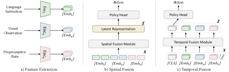
where denotes the feature extractor of each modality. Then, regarding how to process the input , or how to fuse information from multiple modalities into latent representations , we categorize the BC methods in robot manipulation based on feature fusion methods into two types: spatial fusion and temporal fusion.
As illustrated in Figure 2 b), spatial fusion involves extracting spatial features from data at a given time step or concatenating features across multiple time steps along the feature dimensions. This approach does not explicitly differentiate between time steps but instead processes the aggregated features as a whole, emphasizing the modeling of inter-feature relationships. The spatial fusion module can be implemented using Multi-Layer Perceptrons (MLPs), Convolutional Neural Networks (CNNs), Spatial Transformers, or even simple concatenation operations. On the other hand, as illustrated in Figure 2 c), temporal fusion integrates input features by capturing dynamic relationships and dependencies across time steps, enabling the modeling of both long-term and short-term temporal dynamics in sequential data. Temporal fusion modules can be implemented using Recurrent Neural Networks (RNNs), Long Short-Term Memory networks (LSTMs), or Temporal Transformers.
The latent representation , which integrates both spatial and temporal information, is then passed through a policy head to generate actions. Existing policy heads primarily focus on using MLP, Gaussian Mixture Model (GMM), and diffusion-based policy (DP) heads (Chi et al., 2023; Reuss et al., 2024). For simplicity and clearer empirical demonstration, we use an MLP as the policy head.
4.2 Behavior Cloning with Information Bottleneck
The Information Bottleneck (IB) principle is an information-theoretic approach aimed at extracting the most relevant information from an input variable with respect to an output variable, i.e., action . The central idea is to find a compressed representation of that retains the relevant information needed to predict , while discarding irrelevant parts of that do not contribute to predicting . The relevant information is quantified as the mutual information , and the optimal representation is the minimal sufficient statistic of with respect to . In practice, this can be achieved by minimizing a Lagrangian that balances the trade-off between retaining predictive information and compressing the input, which can be formulated as:
| (5) |
where is the Lagrange multiplier that balances the trade-off between the compression ability and the predictive power. Thus Equation 2 can be modified as:
| (6) |
where and denotes the fusion module.
4.3 Theoretical Analysis
We provide a theoretical analysis of our BC-IB objective in Equation 5. Theorem 4.1 and Theorem 4.2 reveal that the generalization error admits an upper bound governed by the mutual information between the input and the latent representation. By minimizing this mutual information, we effectively tighten the upper bound, thereby improving the model’s generalization performance. Theorem 4.3 elucidates the optimization challenges associated with complex input states. When the input contains a large amount of state information, as depicted in Figure 2, directly minimizing the mutual information between and the latent representation becomes computationally impractical. To address this, the input is first compressed into an intermediate embedding via a fusion network , and the mutual information between and is minimized instead. The theorem establishes that, under certain conditions, this intermediate approach can approximate the ideal optimization results, provided that the embedding sufficiently preserves the essential information from the original input .
Theorem 4.1.
Generalization Bound Adapted from (Shwartz-Ziv et al., 2019). Let denote the training data sampled from the same distribution as the random variable pair . Given the policy trained on , the generalization error is given by:
| (7) |
Using the Probably Approximately Correct (PAC) bound framework and the Asymptotic Equipartition Property (AEP) (Cover, 1999), with probability at least , the following upper bound on the generalization error holds:
| (8) |
where represents the mutual information between the input and the intermediate representation , and is the confidence level. Details of proof can be seen in Appendix A of (Shwartz-Ziv et al., 2019).
Theorem 4.2.
Generalization Bound Adapted from (Kawaguchi et al., 2023). Let denote the training data sampled from the same distribution as the random variable pair . The generalization error is approximately bounded by:
| (9) |
where is the encoder mapping the input to the intermediate representation . This bound indicates that the generalization error is:
-
•
Positively correlated with , which captures mutual information between the input and the latent representation , conditioned on the actions . This term reflects that the IB compresses into while preserving the relevant information for predicting .
-
•
Positively correlated with , which reflects the information content of the representation for the given dataset .
Theorem 4.3.
Optimization Gap under Different Input Compression. Let form a Markov chain, where is transformed into by a network , and is further transformed into by a network . Let . Define two optimization problems:
| (10) | ||||
| (11) |
Let .
Assume the mutual information gap satisfies the following, for any have
| (12) |
Then, the gap between the two optimizations is bounded as:
| (13) |
The detailed proof can be found in Appendix A.
5 Experiments
5.1 Embodied Evaluation
Benchmarks. We mainly evaluate BC with IB across two benchmarks, CortexBench (Majumdar et al., 2023) and LIBERO (Liu et al., 2024). CortexBench is a single-task benchmark. For validation, we selected four imitation learning-related simulators, encompassing a total of 14 tasks: Adroit (2 tasks) (Rajeswaran et al., 2018), Meta-World (5 tasks) (Yu et al., 2020), DMControl (5 tasks) (Tassa et al., 2018), and TriFinger (2 tasks) (Wuthrich et al., 2021). During evaluation, the number of validation trajectories is set to 25, 10, 25, and 25, respectively. LIBERO is a language-conditioned multi-task benchmark. For evaluation, we select four suites: LIBERO-Goal (10 tasks), LIBERO-Object (10 tasks), LIBERO-Spatial (10 tasks), and LIBERO-Long (10 tasks), each focusing on the controlled transfer of knowledge related to task goals, objects, spatial information, and long-horizon tasks, respectively. During evaluation, the number of validation trajectories is set to 20.
Baselines. In CortexBench, we evaluate four representation learning models: R3M (Nair et al., 2023), Voltron (Karamcheti et al., 2023), VC-1 (Majumdar et al., 2023), and MPI (Zeng et al., 2024). In line with the original papers, we use the pre-trained versions of these models to facilitate their application to downstream tasks, keeping the image encoders frozen. Additionally, we introduce two full fine-tuning baselines by replacing these encoders with part of uninitialized ResNet-18 (He et al., 2016) and ViT-S (Dosovitskiy, 2021), denoted as ResNet and ViT, respectively. All methods employ the two fusion techniques described in Section 4.1. For spatial fusion, we use an MLP, and for temporal fusion, we utilize a Temporal Transformer. In LIBERO, we implement four vision-language policy networks. One of them uses a spatial fusion approach, which employs ResNet as the image encoder and an MLP as the fusion module, referred to as BC-MLP. The other three use temporal fusion. Following the original paper, we rename them based on the combination of the image encoder and fusion module: BC-RNN, BC-Transformer, and BC-VILT (Liu et al., 2024). The policy head for all methods is fixed as an MLP. Notably, all baselines with IB are referred to as BC+IB.
Implementation. In CortexBench, for four partial fine-tuning methods, we train for 100 epochs on each task using the Adam optimizer with a learning rate of 1e-3, a batch size of 512, and weight decay of 1e-4, with learning rate decay applied using a cosine annealing schedule. For the two full fine-tuning methods, we train for 50 epochs with a learning rate of 1e-4 and a batch size of 256. All other parameters remain unchanged. In LIBERO, we train for 50 epochs using the AdamW optimizer with a learning rate of 1e-4 and a batch size of 64, decayed using a cosine annealing schedule. For BC+IB methods, the model used in MINE consists of a two-layer MLP, with a learning rate of 1e-5. The Lagrange multiplier in Equation 6 ranges from 1e-4 to 5e-3 in this work.
Model Selection. For single-task benchmark CortexBench, we test the model every 5 or 10 epochs and select the model with the highest success rate. For multi-task benchmark LIBERO, we select the model from the final epoch.
The appendix will provide detailed descriptions of each benchmark (Section B.1), all baselines (Section B.2), implementation details (Section B.3), and the rationale behind the model selection (Section B.4).
5.2 Performance on Cortexbench
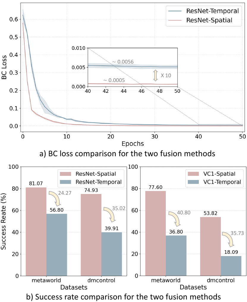
The Selection of Fusion Method. We first evaluate the effectiveness of the two fusion methods in the baselines on CortexBench, with the results shown in Figure 3.
Finding 1: For simple single-task scenarios, spatial fusion is more efficient and effective than temporal fusion. As shown in Figure 3 b), the performance of methods with temporal fusion drops significantly. From Figure 3 a), this can be attributed to the slower loss reduction in methods using temporal fusion, which results in higher loss at the same training epoch. Therefore, we focus exclusively on presenting the results for methods employing spatial fusion.
Results. We next report the performance, i.e., success rate, of the baselines and baselines with IB on the single-task benchmark CortexBench in Table 1 with a full-shot setting. Based on results, we derive the following findings.
Finding 2: Whether using full fine-tuning or partial fine-tuning, all vanilla BC methods with different visual backbones incorporating IB outperform their vanilla counterparts across the board. In some benchmarks, the improvements are substantial. For example, ResNet with IB achieves a 10.01% improvement on DMControl, and VC-1 with IB shows a 4.80% improvement on Meta-World. In Section C.1, we report the success rate for each task, where significant improvements can be observed in certain tasks.
Finding 3: Finding 2 implicitly suggests that the latent representation derived from input is redundant. Therefore, compressing information from input is essential, which can further enhance performance.
Finding 4: For simple single-task downstream tasks, full fine-tuning of a simple, uninitialized model (ResNet) is sufficient and may even outperform a pre-trained larger model. However, the latter is more efficient for faster fine-tuning and deployment, and proves to be more effective for more complex tasks (Burns et al., 2023).
| Method | Image Encoder | Adroit | Meta-World | DMControl | TriFinger | Avg |
| Full Fine-tuning | ||||||
| ResNet (He et al., 2016) | ResNet∗ | 66.005.29 | 81.071.22 | 74.936.21 | 71.590.88 | 73.40 |
| ResNet+IB | 72.002.00 | 83.200.80 | 84.943.54 | 72.301.76 | 78.11 | |
| ViT (Dosovitskiy, 2021) | ViT∗ | 35.333.06 | 31.731.67 | 10.411.21 | 55.572.65 | 33.26 |
| ViT+IB | 37.334.16 | 36.006.97 | 12.532.17 | 55.932.16 | 35.45 | |
| Partial Fine-tuning | ||||||
| R3M (Nair et al., 2023) | ViT-S | 25.336.43 | 53.071.67 | 40.310.65 | 59.870.78 | 44.65 |
| R3M+IB | 27.333.06 | 54.132.44 | 41.745.54 | 60.630.53 | 45.96 | |
| Voltron (Karamcheti et al., 2023) | ViT-S | 18.676.11 | 72.531.22 | 25.352.81 | 74.212.61 | 47.69 |
| Voltron+IB | 21.335.77 | 74.403.49 | 33.166.70 | 75.122.47 | 51.00 | |
| VC-1 (Majumdar et al., 2023) | ViT-B | 24.677.02 | 77.602.88 | 53.825.03 | 72.052.17 | 57.04 |
| VC-1+IB | 26.009.17 | 82.402.88 | 54.931.11 | 73.801.27 | 59.28 | |
| MPI (Zeng et al., 2024) | ViT-S | 34.674.16 | 66.402.12 | 59.451.91 | 61.910.57 | 55.61 |
| MPI+IB | 36.676.11 | 69.331.67 | 61.413.15 | 63.341.52 | 57.69 | |
| Method | Image Encoder | Fuse Module | LIBERO-Goal | LIBERO-Object | LIBERO-Spatial | LIBERO-Long | Avg |
|---|---|---|---|---|---|---|---|
| BC-MLP | ResNet | MLP | 16.503.97 | 19.0012.22 | 29.339.61 | 2.330.76 | 16.79 |
| BC-MLP+IB | 27.6712.00 | 31.5010.83 | 41.008.32 | 2.670.76 | 25.71 | ||
| BC-RNN | ResNet | RNN | 15.1710.91 | 13.337.91 | 30.6713.34 | 2.330.67 | 15.38 |
| BC-RNN+IB | 26.003.50 | 17.675.77 | 35.179.45 | 3.000.17 | 20.46 | ||
| BC-Trans. | ResNet | T-Trans. | 67.8310.42 | 41.831.89 | 68.001.00 | 15.832.52 | 48.37 |
| BC-Trans.+IB | 74.175.75 | 45.674.31 | 72.5010.26 | 18.006.38 | 52.59 | ||
| BC-VILT | S-Trans. | T-Trans. | 76.173.01 | 43.003.91 | 67.172.25 | 6.500.87 | 48.21 |
| BC+VILT+IB | 83.833.40 | 52.003.04 | 70.672.52 | 8.671.53 | 53.79 |
5.3 Performance on LIBERO
Results. We report the performance on the multi-task benchmark LIBERO with a full-shot setting in Table 2.
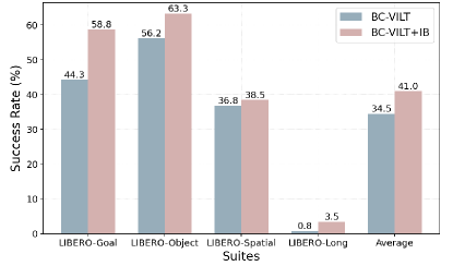
Finding 5: For more complex language-conditioned multi-task scenarios, all baselines with different backbones incorporating IB consistently show performance improvements across all LIBERO benchmarks. For example, BC-VILT achieves large gains of 7.66% and 9.00% on LIBERO-Goal and LIBERO-Object, respectively, while BC-RNN shows a significant improvement of 10.83% on LIBERO-Goal. IB proves to be more effective in more complex environments and settings. We attribute this to the difference in task complexity: in CortexBench, the history length is 3, while in LIBERO, it is 10, with LIBERO being a multi-task benchmark and CortexBench being single-task benchmark. The increased data complexity (task quantity and input information) suggests a higher level of data redundancy, making IB even more effective.
Finding 6: We observe that in complex multi-task scenarios with more intricate inputs, such as a greater number of input modalities and extended historical information, using the Temporal Transformer in temporal fusion proves to be more effective than both spatial fusion and RNN-based temporal fusion. The evidence lies in the fact that the average success rates of BC-Transfomer and BC-VILT are over 30% higher than those of BC-MLP and BC-RNN. This is likely because Temporal Transformers excel in handling long-range interactions and capture dynamic dependencies across time steps, where RNNs and spatial fusion methods may struggle. This finding, together with Finding 1, underscores the specific scenarios in which each fusion method is most applicable.
Finding 7: IB is particularly effective for tasks requiring diverse feature extraction, such as distinguishing distinct task objectives or differentiating between various objects, as in LIBERO-Goal and LIBERO-Object. By filtering out irrelevant information, IB facilitates better generalization and more compact representations. However, its impact is less pronounced in spatial and long-horizon tasks, such as LIBERO-Spatial and LIBERO-Long, which heavily depend on structural and sequential dependencies that may be disrupted by excessive compression.
5.4 More Analysis
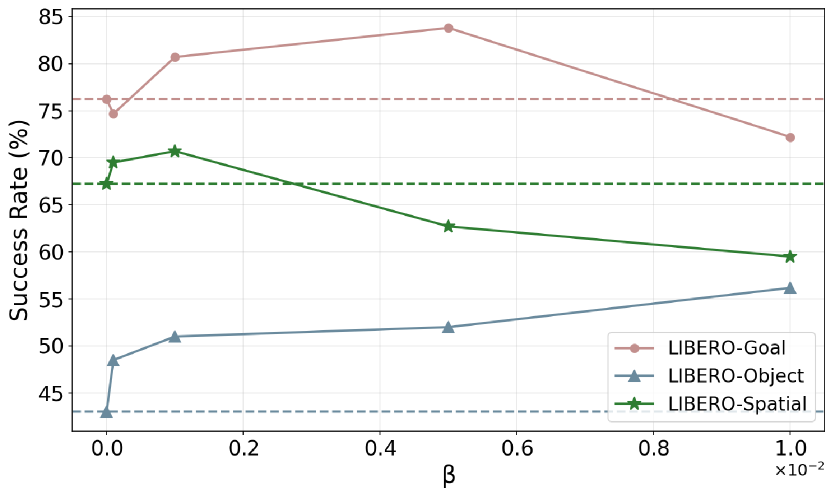
Effect of the Lagrange multiplier of Equation 6. This experiment evaluates how incorporating IB enhances performance. Since the MINE model’s parameters are fixed, the key difference between BC+IB and BC lies in the parameter , which balances compression and predictive power. For LIBERO experiments, is explored within 1e-4, 1e-3, 5e-3, 1e-2. Finding 8: As shown in Figure 5, IB improves performance within a specific range, with a peak observed at an undetermined value. However, across all experiments, around 1e-4 consistently yields stable improvements. The selected values for each experiment are detailed in C.1.
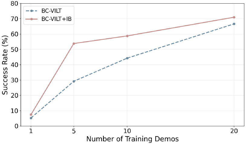
Effect of the Number of Demonstrations. We evaluate IB’s effectiveness in few-shot settings, as few-shot learning is crucial for fine-tuning on domain-specific tasks in real-world applications. Finding 9: As shown in Figure 6, IB significantly improves performance even with limited data, highlighting its effectiveness in real-world scenarios where data is scarce. This further underscores the potential of IB in improving model generalization in practical settings.
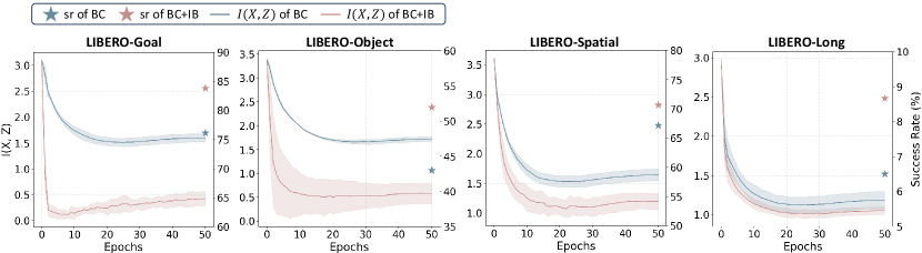
Visualizations of . As shown in Figure 4, BC+IB achieves a greater reduction in compared to vanilla BC, leading to significant performance improvements and further validating the effectiveness of IB. For instance, in LIBERO-Goal, incorporating IB reduces to one-quarter of its original value, resulting in a 7.7% increase in success rate.
We provide real-world experiments in Section C.2.
6 Limitations and Discussion
While our work provides extensive experimental validation of the effectiveness of IB and the necessity of input redundancy reduction in robotics representation learning, several limitations remain. First, for scalability, we do not incorporate large models like vision-language-action models due to high computational and time costs. Consequently, architectures like RT-2 (Brohan et al., 2023) and OpenVLA (Kim et al., 2024), which forgo a policy head and treat actions as text tokens, have not been explored. This is an avenue we aim to investigate in future work. Second, we have not examined alternative policy heads, such as diffusion-based (Chi et al., 2023) or transformer-based policy heads (Octo Model Team et al., 2024), which may further enhance performance. Third, while we evaluate our method on controlled benchmarks, its robustness to domain shifts, such as environmental or task variations, remains underexplored. We hope our work will inspire future research and contribute to the ongoing development and refinement of these methods.
7 Conclusions
In this study, we investigated the redundancy in representations for Behavior Cloning in robot manipulation and introduced the Information Bottleneck principle to mitigate this issue. By incorporating IB, we aimed to filter out redundant information in latent representations while preserving task-relevant features. Extensive experiments across various representation learning methods on CortexBench and LIBERO revealed insightful findings and demonstrated that IB significantly improves performance across diverse tasks and architectures. We hope our work will inspire further integration of information-theoretic principles into robotics and foster deeper theoretical analysis in this domain.
Acknowledgements
This work was supported by the National Natural Science Foundation of China with grant numbers (U21A20485 and 62436005), and the Fundamental Research Funds for Xi’an Jiaotong University under Grants xzy022024012.
References
- Argall et al. (2009) Argall, B. D., Chernova, S., Veloso, M., and Browning, B. A survey of robot learning from demonstration. Robotics and autonomous systems, 57(5):469–483, 2009.
- Bai et al. (2021) Bai, C., Wang, L., Han, L., Garg, A., Hao, J., Liu, P., and Wang, Z. Dynamic bottleneck for robust self-supervised exploration. Advances in Neural Information Processing Systems, 34:17007–17020, 2021.
- Bain & Sammut (1995) Bain, M. and Sammut, C. A framework for behavioural cloning. In Machine Intelligence 15, pp. 103–129, 1995.
- Bardera et al. (2009) Bardera, A., Rigau, J., Boada, I., Feixas, M., and Sbert, M. Image segmentation using information bottleneck method. IEEE Transactions on Image Processing, 18(7):1601–1612, 2009.
- Belghazi et al. (2018) Belghazi, M. I., Baratin, A., Rajeshwar, S., Ozair, S., Bengio, Y., Courville, A., and Hjelm, D. Mutual information neural estimation. In International conference on machine learning, pp. 531–540. PMLR, 2018.
- Brohan et al. (2023) Brohan, A., Brown, N., Carbajal, J., Chebotar, Y., Chen, X., Choromanski, K., Ding, T., Driess, D., Dubey, A., Finn, C., et al. Rt-2: Vision-language-action models transfer web knowledge to robotic control. In Conference on Robot Learning, 2023.
- Burns et al. (2023) Burns, K., Witzel, Z., Hamid, J. I., Yu, T., Finn, C., and Hausman, K. What makes pre-trained visual representations successful for robust manipulation? arXiv preprint arXiv:2312.12444, 2023.
- Cheang et al. (2024) Cheang, C.-L., Chen, G., Jing, Y., Kong, T., Li, H., Li, Y., Liu, Y., Wu, H., Xu, J., Yang, Y., et al. Gr-2: A generative video-language-action model with web-scale knowledge for robot manipulation. arXiv preprint arXiv:2410.06158, 2024.
- Chi et al. (2023) Chi, C., Xu, Z., Feng, S., Cousineau, E., Du, Y., Burchfiel, B., Tedrake, R., and Song, S. Diffusion policy: Visuomotor policy learning via action diffusion. The International Journal of Robotics Research, pp. 02783649241273668, 2023.
- Cover (1999) Cover, T. M. Elements of information theory. John Wiley & Sons, 1999.
- Deng et al. (2009) Deng, J., Dong, W., Socher, R., Li, L.-J., Li, K., and Fei-Fei, L. Imagenet: A large-scale hierarchical image database. In 2009 IEEE conference on computer vision and pattern recognition, pp. 248–255. Ieee, 2009.
- Donsker & Varadhan (1983) Donsker, M. D. and Varadhan, S. S. Asymptotic evaluation of certain markov process expectations for large time. iv. Communications on pure and applied mathematics, 36(2):183–212, 1983.
- Dosovitskiy (2021) Dosovitskiy, A. An image is worth 16x16 words: Transformers for image recognition at scale. 2021.
- Federici et al. (2019) Federici, M., Dutta, A., Forré, P., Kushman, N., and Akata, Z. Learning robust representations via multi-view information bottleneck. In International Conference on Learning Representations, 2019.
- Goyal et al. (2023) Goyal, A., Xu, J., Guo, Y., Blukis, V., Chao, Y.-W., and Fox, D. Rvt: Robotic view transformer for 3d object manipulation. In Conference on Robot Learning, pp. 694–710. PMLR, 2023.
- Grauman et al. (2022) Grauman, K., Westbury, A., Byrne, E., Chavis, Z., Furnari, A., Girdhar, R., Hamburger, J., Jiang, H., Liu, M., Liu, X., et al. Ego4d: Around the world in 3,000 hours of egocentric video. In Proceedings of the IEEE/CVF Conference on Computer Vision and Pattern Recognition, pp. 18995–19012, 2022.
- He et al. (2024) He, H., Wu, P., Bai, C., Lai, H., Wang, L., Pan, L., Hu, X., and Zhang, W. Bridging the sim-to-real gap from the information bottleneck perspective. In 8th Annual Conference on Robot Learning, 2024.
- He et al. (2016) He, K., Zhang, X., Ren, S., and Sun, J. Deep residual learning for image recognition. In Proceedings of the IEEE conference on computer vision and pattern recognition, pp. 770–778, 2016.
- He et al. (2022) He, K., Chen, X., Xie, S., Li, Y., Dollár, P., and Girshick, R. Masked autoencoders are scalable vision learners. In Proceedings of the IEEE/CVF conference on computer vision and pattern recognition, pp. 16000–16009, 2022.
- Hu et al. (2024) Hu, Y., Guo, Y., Wang, P., Chen, X., Wang, Y.-J., Zhang, J., Sreenath, K., Lu, C., and Chen, J. Video prediction policy: A generalist robot policy with predictive visual representations. arXiv preprint arXiv:2412.14803, 2024.
- Jang et al. (2022) Jang, E., Irpan, A., Khansari, M., Kappler, D., Ebert, F., Lynch, C., Levine, S., and Finn, C. Bc-z: Zero-shot task generalization with robotic imitation learning. In Conference on Robot Learning, pp. 991–1002. PMLR, 2022.
- Jeon et al. (2021) Jeon, I., Lee, W., Pyeon, M., and Kim, G. Ib-gan: Disentangled representation learning with information bottleneck generative adversarial networks. In Proceedings of the AAAI conference on artificial intelligence, volume 35, pp. 7926–7934, 2021.
- Jia et al. (2024) Jia, Z., Thumuluri, V., Liu, F., Chen, L., Huang, Z., and Su, H. Chain-of-thought predictive control. In Forty-first International Conference on Machine Learning, 2024.
- Karamcheti et al. (2023) Karamcheti, S., Nair, S., Chen, A. S., Kollar, T., Finn, C., Sadigh, D., and Liang, P. Language-driven representation learning for robotics. In Robotics: Science and Systems, 2023.
- Kawaguchi et al. (2023) Kawaguchi, K., Deng, Z., Ji, X., and Huang, J. How does information bottleneck help deep learning? In International Conference on Machine Learning, pp. 16049–16096. PMLR, 2023.
- Kim et al. (2024) Kim, M. J., Pertsch, K., Karamcheti, S., Xiao, T., Balakrishna, A., Nair, S., Rafailov, R., Foster, E., Lam, G., Sanketi, P., et al. Openvla: An open-source vision-language-action model. arXiv preprint arXiv:2406.09246, 2024.
- Kim et al. (2019) Kim, Y., Nam, W., Kim, H., Kim, J.-H., and Kim, G. Curiosity-bottleneck: Exploration by distilling task-specific novelty. In International conference on machine learning, pp. 3379–3388. PMLR, 2019.
- Lee et al. (2021) Lee, J., Choi, J., Mok, J., and Yoon, S. Reducing information bottleneck for weakly supervised semantic segmentation. Advances in neural information processing systems, 34:27408–27421, 2021.
- Liu et al. (2024) Liu, B., Zhu, Y., Gao, C., Feng, Y., Liu, Q., Zhu, Y., and Stone, P. Libero: Benchmarking knowledge transfer for lifelong robot learning. Advances in Neural Information Processing Systems, 36, 2024.
- Ma et al. (2024) Ma, T., Zhou, J., Wang, Z., Qiu, R., and Liang, J. Contrastive imitation learning for language-guided multi-task robotic manipulation. 2024.
- Majumdar et al. (2023) Majumdar, A., Yadav, K., Arnaud, S., Ma, J., Chen, C., Silwal, S., Jain, A., Berges, V.-P., Wu, T., Vakil, J., et al. Where are we in the search for an artificial visual cortex for embodied intelligence? Advances in Neural Information Processing Systems, 36:655–677, 2023.
- Nair et al. (2023) Nair, S., Rajeswaran, A., Kumar, V., Finn, C., and Gupta, A. R3m: A universal visual representation for robot manipulation. In Conference on Robot Learning, pp. 892–909. PMLR, 2023.
- Octo Model Team et al. (2024) Octo Model Team, Ghosh, D., Walke, H., Pertsch, K., Black, K., Mees, O., Dasari, S., Hejna, J., Xu, C., Luo, J., Kreiman, T., Tan, Y., Sanketi, P., Vuong, Q., Xiao, T., Sadigh, D., Finn, C., and Levine, S. Octo: An open-source generalist robot policy. 2024.
- Pearce & Zhu (2022) Pearce, T. and Zhu, J. Counter-strike deathmatch with large-scale behavioural cloning. In 2022 IEEE Conference on Games (CoG), pp. 104–111. IEEE, 2022.
- Perez et al. (2018) Perez, E., Strub, F., De Vries, H., Dumoulin, V., and Courville, A. Film: Visual reasoning with a general conditioning layer. In Proceedings of the AAAI conference on artificial intelligence, volume 32, 2018.
- Pomerleau (1991) Pomerleau, D. A. Efficient training of artificial neural networks for autonomous navigation. Neural computation, 3(1):88–97, 1991.
- Radosavovic et al. (2023) Radosavovic, I., Xiao, T., James, S., Abbeel, P., Malik, J., and Darrell, T. Real-world robot learning with masked visual pre-training. In Conference on Robot Learning, pp. 416–426. PMLR, 2023.
- Rajeswaran et al. (2018) Rajeswaran, A., Kumar, V., Gupta, A., Vezzani, G., Schulman, J., Todorov, E., and Levine, S. Learning complex dexterous manipulation with deep reinforcement learning and demonstrations. Robotics: Science and Systems, 2018.
- Reuss et al. (2024) Reuss, M., Yağmurlu, Ö. E., Wenzel, F., and Lioutikov, R. Multimodal diffusion transformer: Learning versatile behavior from multimodal goals. In First Workshop on Vision-Language Models for Navigation and Manipulation at ICRA 2024, 2024.
- Saxena et al. (2025) Saxena, V., Bronars, M., Arachchige, N. R., Wang, K., Shin, W. C., Nasiriany, S., Mandlekar, A., and Xu, D. What matters in learning from large-scale datasets for robot manipulation. In International Conference on Learning Representations, 2025.
- Shwartz-Ziv et al. (2019) Shwartz-Ziv, R., Painsky, A., and Tishby, N. REPRESENTATION COMPRESSION AND GENERALIZATION IN DEEP NEURAL NETWORKS, 2019. URL https://openreview.net/forum?id=SkeL6sCqK7.
- Tassa et al. (2018) Tassa, Y., Doron, Y., Muldal, A., Erez, T., Li, Y., Casas, D. d. L., Budden, D., Abdolmaleki, A., Merel, J., Lefrancq, A., et al. Deepmind control suite. arXiv preprint arXiv:1801.00690, 2018.
- Tian et al. (2025) Tian, Y., Yang, S., Zeng, J., Wang, P., Lin, D., Dong, H., and Pang, J. Predictive inverse dynamics models are scalable learners for robotic manipulation. 2025.
- Tishby et al. (1999) Tishby, N., Pereira, F. C., and Bialek, W. The information bottleneck method. arXiv preprint physics/0004057, 1999.
- Torabi et al. (2018) Torabi, F., Warnell, G., and Stone, P. Behavioral cloning from observation. In Proceedings of the 27th International Joint Conference on Artificial Intelligence, pp. 4950–4957, 2018.
- Vaswani (2017) Vaswani, A. Attention is all you need. Advances in Neural Information Processing Systems, 2017.
- Wang et al. (2024) Wang, L., Chen, X., Zhao, J., and He, K. Scaling proprioceptive-visual learning with heterogeneous pre-trained transformers. 2024.
- Wen et al. (2020) Wen, C., Lin, J., Darrell, T., Jayaraman, D., and Gao, Y. Fighting copycat agents in behavioral cloning from observation histories. Advances in Neural Information Processing Systems, 33:2564–2575, 2020.
- Wen et al. (2024) Wen, C., Lin, X., So, J., Chen, K., Dou, Q., Gao, Y., and Abbeel, P. Any-point trajectory modeling for policy learning. In Robotics: Science and Systems, 2024.
- Wuthrich et al. (2021) Wuthrich, M., Widmaier, F., Grimminger, F., Joshi, S., Agrawal, V., Hammoud, B., Khadiv, M., Bogdanovic, M., Berenz, V., Viereck, J., et al. Trifinger: An open-source robot for learning dexterity. In Conference on Robot Learning, pp. 1871–1882. PMLR, 2021.
- Yu et al. (2020) Yu, T., Quillen, D., He, Z., Julian, R., Hausman, K., Finn, C., and Levine, S. Meta-world: A benchmark and evaluation for multi-task and meta reinforcement learning. In Conference on robot learning, pp. 1094–1100. PMLR, 2020.
- Zawalski et al. (2024) Zawalski, M., Chen, W., Pertsch, K., Mees, O., Finn, C., and Levine, S. Robotic control via embodied chain-of-thought reasoning. In 8th Annual Conference on Robot Learning, 2024.
- Ze et al. (2024) Ze, Y., Zhang, G., Zhang, K., Hu, C., Wang, M., and Xu, H. 3d diffusion policy: Generalizable visuomotor policy learning via simple 3d representations. In ICRA 2024 Workshop on 3D Visual Representations for Robot Manipulation, 2024.
- Zeng et al. (2024) Zeng, J., Bu, Q., Wang, B., Xia, W., Chen, L., Dong, H., Song, H., Wang, D., Hu, D., Luo, P., et al. Learning manipulation by predicting interaction. 2024.
- Zhu et al. (2024) Zhu, H., Yang, H., Wang, Y., Yang, J., Wang, L., and He, T. Spa: 3d spatial-awareness enables effective embodied representation. arXiv preprint arXiv:2410.08208, 2024.
Appendix A Proof of Theorem 4.3
Proof.
The first optimization problem optimizes , which imposes a looser constraint on , as it does not directly regulate the information flow from to . In contrast, the second optimization problem directly constrains , which may result in a smaller . Therefore, we have:
| (14) |
From the optimization objectives of the two problems, it follows that:
| (15) |
Rearranging this inequality gives:
| (16) |
According to the assumption that the mutual information gap is bounded:
| (17) |
we substitute this bound into the inequality:
| (18) |
Thus, the performance gap is bounded as:
| (19) |
This completes the proof. ∎
Appendix B Details of Experiment Setting
B.1 Details of Benchmarks
B.1.1 CortexBench
We provide a detailed overview of the four imitation learning benchmarks used in CortexBench (Majumdar et al., 2023). CortexBench is a single-task benchmark that includes 7 selected simulators, collectively offering 17 different embodied AI tasks spanning locomotion, navigation, and both dexterous and mobile manipulation. Three of the simulators are related to reinforcement learning, and thus are excluded from our analysis. The remaining four simulators, with a total of 14 tasks, are retained for validation: Adroit (2 tasks) (Rajeswaran et al., 2018), Meta-World (5 tasks) (Yu et al., 2020), DMControl (5 tasks) (Tassa et al., 2018), and TriFinger (2 tasks) (Wuthrich et al., 2021).
First, Adroit (Rajeswaran et al., 2018) is a suite of dexterous manipulation tasks in which an agent controls a 28-DoF anthropomorphic hand. It includes two of the most challenging tasks: Relocate and Reorient-Pen. In these tasks, the agent must manipulate an object to achieve a specified goal position and orientation. Each task consists of 100 demonstrations.
Second, MetaWorld (Yu et al., 2020) is a collection of tasks in which agents command a Sawyer robot arm to manipulate objects in a tabletop environment. CortexBench includes five tasks from MetaWorld: Assembly, Bin-Picking, Button-Press, Drawer-Open, and Hammer. Each task consists of 25 demonstrations.
Third, DeepMind Control (DMControl) (Tassa et al., 2018) is a widely studied image-based continuous control benchmark, where agents perform locomotion and object manipulation tasks. CortexBench includes five DMC tasks: Finger-Spin, Reacher-Hard, Cheetah-Run, Walker-Stand, and Walker-Walk. Each task consists of 100 demonstrations.
Lastly, TriFinger (TF) (Wuthrich et al., 2021) is a robot consisting of a three-finger hand with 3-DoF per finger. CortexBench includes two tasks from TriFinger: Push-Cube and Reach-Cube. Each task consists of 100 demonstrations.
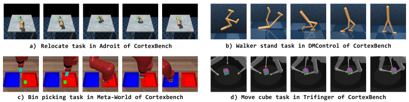
Although only Meta-World is strictly a robot manipulation benchmark, we include all tasks to demonstrate the effectiveness of IB comprehensively. We provide visualizations for one task from each benchmark, as shown in Figure 7.
B.1.2 LIEBRO
LIBERO is a language-conditioned multi-task benchmark comprising 130 tasks across five suites. LIBERO (Liu et al., 2024) has four task suites: LIBERO-Goal (10 tasks), LIBERO-Object (10 tasks), LIBERO-Spatial (10 tasks), and LIBERO-100 (100 tasks).
LIBERO-Goal tasks share the same objects with fixed spatial relationships but differ in task goals, requiring the robot to continually acquire new knowledge about motions and behaviors. Examples include (1) opening the middle drawer of the cabinet, (2) opening the top drawer and placing the bowl inside, (3) pushing the plate to the front of the stove, (4) placing the bowl on the plate, (5) placing the bowl on the stove, (6) placing the bowl on top of the cabinet, (7) placing the cream cheese in the bowl, (8) placing the wine bottle on the rack, (9) placing the wine bottle on top of the cabinet, and (10) turning on the stove.
LIBERO-Object tasks involve the robot picking and placing unique objects, requiring it to continually learn and memorize new object types. Examples include (1) picking up the alphabet soup and placing it in the basket, (2) picking up the BBQ sauce and placing it in the basket, (3) picking up the butter and placing it in the basket, (4) picking up the chocolate pudding and placing it in the basket, (5) picking up the cream cheese and placing it in the basket, (6) picking up the ketchup and placing it in the basket, (7) picking up the milk and placing it in the basket, (8) picking up the orange juice and placing it in the basket, (9) picking up the salad dressing and placing it in the basket, and (10) picking up the tomato sauce and placing it in the basket.
LIBERO-Spatial requires the robot to place a bowl, selected from the same set of objects, onto a plate. The robot must continually learn and memorize new spatial relationships. Examples include (1) picking up the black bowl between the plate and the ramekin and placing it on the plate, (2) picking up the black bowl from the table center and placing it on the plate, (3) picking up the black bowl in the top drawer of the wooden cabinet and placing it on the plate, (4) picking up the black bowl next to the cookie box and placing it on the plate, (5) picking up the black bowl next to the plate and placing it on the plate, (6) picking up the black bowl next to the ramekin and placing it on the plate, (7) picking up the black bowl on the cookie box and placing it on the plate, (8) picking up the black bowl on the ramekin and placing it on the plate, (9) picking up the black bowl on the stove and placing it on the plate, and (10) picking up the black bowl on the wooden cabinet and placing it on the plate.
LIBERO-100 consists of 100 tasks involving diverse object interactions and versatile motor skills. It can be divided into LIBERO-10 (10 tasks) and LIBERO-90 (90 tasks), where we use LIBERO-10, also referred to as LIBERO-Long, as our benchmark. LIBERO-Long requires the robot to learn long-horizon tasks, demanding it to plan and execute actions over extended periods to accomplish complex objectives. Examples include (1) turning on the stove and placing the moka pot on it, (2) putting the black bowl in the bottom drawer of the cabinet and closing it, (3) putting the yellow and white mug in the microwave and closing it, (4) putting both moka pots on the stove, (5) putting both the alphabet soup and the cream cheese box in the basket, (6) putting both the alphabet soup and the tomato sauce in the basket, (7) putting the cream cheese box and the butter in the basket, (8) putting the white mug on the left plate and the yellow and white mug on the right plate, (9) putting the white mug on the plate and the chocolate pudding to the right of the plate, and (10) picking up the book and placing it in the back compartment of the caddy.
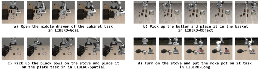
We provide visualizations for one task from each suite, as shown in Figure 8.
B.2 Details of Baselines
B.2.1 Baselines in CortexBench
In CortexBench, the classification of baselines is primarily based on the visual encoder used.
For full fine-tuning baselines, ResNet (He et al., 2016) and ViT (Dosovitskiy, 2021) are baselines built from the original ResNet-18 and ViT-S models, using only a portion of their architecture and with uninitialized parameters.
For partial fine-tuning baselines, R3M (Nair et al., 2023) pre-trains a ResNet model on human videos (Grauman et al., 2022) using time contrastive learning and video-language alignment. For direct comparison, we use the version reproduced with ViT. VC-1 (Majumdar et al., 2023) pre-trains a ViT using Masked Auto-Encoding (MAE) (He et al., 2022) on a mix of human-object interaction videos, navigation, and the ImageNet (Deng et al., 2009) datasets. Voltron (Karamcheti et al., 2023), a framework for language-driven representation learning from human videos and associated captions, pre-trains a ViT using MAE. MPI (Zeng et al., 2024), a framework for interaction-oriented representation learning, directs the model to predict transition frames and detect manipulated objects using keyframes as input. It learns from human videos and associated captions.
If a proprioceptive state is available, it is first transformed into embeddings using a linear layer. Depending on the fusion method, these embeddings are then combined with the visual embeddings. For spatial fusion, an MLP is used, while for temporal fusion, a temporal transformer is employed. The fused features are ultimately processed through an MLP-based policy head to generate actions.
B.2.2 Baselines in LEBERO
Similar to previous work (Zhu et al., 2024), the baselines in LIBERO largely follow the three architectures outlined in the original paper (Liu et al., 2024), which we have renamed as BC-RNN, BC-Transformer, and BC-VILT. These three baselines are part of the temporal fusion methods.
BC-RNN uses a ResNet as the visual backbone to encode per-step visual observations, with an LSTM as the temporal backbone to process a sequence of encoded visual information. The language instruction is incorporated into the ResNet features using the FiLM method (Perez et al., 2018), and is added to the LSTM inputs.
BC-Transformer employs a similar ResNet-based visual backbone but instead uses a transformer decoder (Vaswani, 2017) as the temporal backbone to process outputs from ResNet, which are temporal sequences of visual tokens. The language embedding is treated as a separate token alongside the visual tokens in the input to the transformer.
BC-VILT utilizes a ViT as the visual backbone and a transformer decoder as the temporal backbone. The language embedding is treated as a separate token in the inputs of both the ViT and the transformer decoder. All temporal backbones output a latent vector at each decision-making step.
Additionally, we introduce a spatial fusion method, BC-MLP, which uses a similar ResNet-based visual backbone. The visual and language embeddings are directly concatenated and input into an MLP for fusion. After feature fusion, all methods use an MLP-based policy head to generate actions.
| Hyperparameters | Training |
|---|---|
| epoch | 50 100 |
| batch size | 256 512 |
| optimizer | AdamW |
| learning rate | 1e-4 1e-3 |
| weight decay | 1e-4 |
| lr scheduler | Cosine |
| lr warm up | 0 |
| clip grad | 100 |
| augmentation | Resize, CenterCrop, Normalize |
| history length | 3 |
| Hyperparameters | Training |
|---|---|
| epoch | 50 |
| batch size | 64 |
| optimizer | AdamW |
| learning rate | 1e-4 |
| weight decay | 1e-4 |
| lr scheduler | Cosine |
| lr warm up | 0 |
| clip grad | 100 |
| augmentation | Normalize, ColorJitter |
| history length | 10 |
| IB-related Hyperparameters | Training |
|---|---|
| MINE model | |
| architecture | 4-layer MLP |
| hidden size | 512 |
| output size | 1 |
| optimizer | Adam |
| learning rate | 1e-5 |
| loss weight | 0.1 |
| IB loss | |
| Lagrange multiplier | [1e-4, 5e-3] |
B.3 Details of Implementations
For all experiments, we use a single Nvidia V100 GPU (CUDA 11.3) with 12 CPUs for training and evaluation.
B.3.1 CortexBench
We largely adhere to the original parameter settings from the CortexBench paper (Majumdar et al., 2023). For both full fine-tuning and partial fine-tuning methods, as shown in Table 4, training parameters are presented with full fine-tuning on the left and partial fine-tuning on the right. For model architecture parameters, spatial fusion employs a 4-layer MLP, where the input dimension matches the output dimension of the image encoder. The features are first downsampled and then upsampled to maintain consistency with the input dimension. For temporal fusion, each modality’s feature dimension is first projected to 64, then processed through a four-layer, six-head Transformer. For dataset configurations, we adopt a full-shot setting, training with 100 demonstrations for Adroit, 100 for DMControl, 25 for MetaWorld, and 100 for TriFinger. During evaluation, we assess performance using 25, 10, 25, and 25 test trajectories, respectively.
B.3.2 LIBERO
We largely follow the original parameter settings from the LIBERO paper (Liu et al., 2024). The training parameters are provided in Table 4. Regarding model architecture, Appendix A.1 of the original LIBERO paper (Liu et al., 2024) describes the model parameters for BC-RNN, BC-Transformer, and BC-VILT. Here, we present the model parameters for BC-MLP, which shares the same architecture as BC-Transformer except for the fusion module. Specifically, BC-MLP employs a four-layer MLP with a hidden size of 256 as its fusion module. For dataset configurations, in the full-shot setting, we use five demonstrations for evaluation, leaving the remaining 45 for training, which is considered the full-shot setting in our experiments. However, full-shot training typically refers to utilizing all 50 demonstrations without allocating any for evaluation, as robotic systems can operate without separate validation data.
For BC+IB, all training and model parameters remain identical to those of BC, except for the IB-specific parameters. The details of IB-related parameters are provided in Table 5, while the specific values of the Lagrange multiplier are thoroughly discussed in Section C.1.
B.4 Details of Model Selection
B.4.1 CortexBench
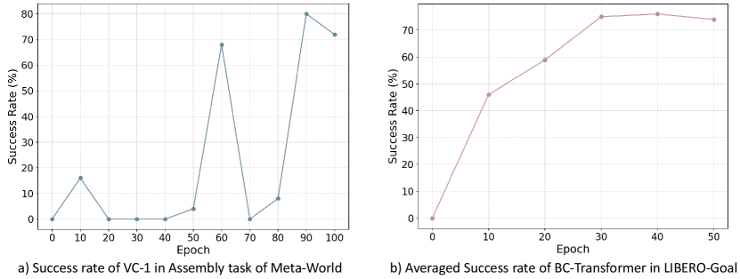
In the single-task dataset CortexBench, we observed that the learning curves of certain tasks exhibit significant oscillations, such as the assemble task in MetaWorld, as shown in Figure 9 a). Previous studies often record performance at intervals of many epochs or steps, selecting either the highest value (Majumdar et al., 2023) or the average of multiple peak values (Ze et al., 2024). Following (Majumdar et al., 2023), we directly use the highest value to explore the model’s full potential on the given task.
B.4.2 LIBERO
For the multi-task dataset LIBERO, we observed that while the learning curve for individual tasks may still oscillate, a decrease in success rate for one task is often accompanied by an increase for another. This trade-off results in smoother overall learning curves across multiple tasks, as shown in Figure 9 b). To make model selection more practical and representative, we directly select the model from the final epoch.
| Adroit | TriFinger | ||||||
|---|---|---|---|---|---|---|---|
| Method | Reorient-Pen | Relocate | Avg | Reach-Cube | Move-Cube | Avg | |
| ResNet | sr | 65.33 | 66.67 | 66.00 | 87.12 | 56.06 | 71.59 |
| ResNet+IB | sr | 69.33 | 74.67 | 72.00 | 87.14 | 57.45 | 72.30 |
| 5e-3 | 1e-4 | 5e-3 | 5e-3 | ||||
| ViT | sr | 61.33 | 9.33 | 35.33 | 78.77 | 32.37 | 55.57 |
| ViT+IB | sr | 64.00 | 10.67 | 37.33 | 77.83 | 34.04 | 55.93 |
| 5e-3 | 5e-3 | 5e-3 | 5e-3 | ||||
| R3M | sr | 45.33 | 5.33 | 25.33 | 74.29 | 45.45 | 59.87 |
| R3M+IB | sr | 52.00 | 2.67 | 27.33 | 75.04 | 46.23 | 60.63 |
| 5e-3 | 5e-3 | 5e-3 | 5e-3 | ||||
| Voltron | sr | 32.00 | 5.33 | 18.67 | 86.37 | 62.04 | 74.21 |
| Voltron+IB | sr | 38.67 | 4.00 | 21.33 | 86.62 | 63.61 | 75.12 |
| 5e-3 | 5e-3 | 5e-3 | 5e-3 | ||||
| VC-1 | sr | 38.67 | 10.67 | 24.67 | 84.19 | 59.90 | 72.05 |
| VC-1+IB | sr | 37.33 | 14.67 | 26.00 | 84.69 | 62.91 | 73.80 |
| 1e-3 | 1e-3 | 5e-3 | 5e-3 | ||||
| MPI | sr | 60.00 | 9.33 | 34.67 | 79.69 | 44.13 | 61.91 |
| MPI+IB | sr | 61.33 | 12.00 | 36.67 | 79.91 | 46.78 | 63.34 |
| 1e-4 | 1e-4 | 5e-3 | 5e-3 | ||||
| Method | Cheetah-Run | Finger-Spin | Reacher-Easy | Walker-Stand | Walker-Walk | Avg | |
|---|---|---|---|---|---|---|---|
| ResNet | sr | 38.32 | 88.37 | 92.20 | 91.42 | 64.34 | 74.93 |
| ResNet+IB | sr | 50.75 | 90.42 | 99.78 | 96.39 | 87.37 | 84.94 |
| 1e-3 | 1e-3 | 1e-3 | 1e-3 | 1e-3 | |||
| ViT | sr | 7.22 | 3.39 | 18.97 | 18.05 | 4.43 | 10.41 |
| ViT+IB | sr | 4.27 | 12.34 | 24.11 | 17.45 | 4.46 | 12.53 |
| 1e-3 | 1e-3 | 1e-3 | 1e-3 | 1e-3 | |||
| R3M | sr | 17.01 | 65.31 | 53.73 | 49.25 | 16.27 | 40.31 |
| R3M+IB | sr | 16.19 | 72.10 | 57.34 | 46.48 | 16.60 | 41.74 |
| 1e-3 | 1e-3 | 1e-3 | 1e-3 | 1e-3 | |||
| Voltron | sr | 1.65 | 8.56 | 44.06 | 46.27 | 26.19 | 25.35 |
| Voltron+IB | sr | 6.93 | 23.85 | 35.89 | 56.48 | 42.68 | 33.16 |
| 1e-3 | 1e-3 | 1e-3 | 1e-3 | 1e-3 | |||
| VC-1 | sr | 20.02 | 85.35 | 74.01 | 64.65 | 25.07 | 53.82 |
| VC-1+IB | sr | 21.52 | 80.91 | 74.80 | 67.10 | 30.34 | 54.93 |
| 1e-3 | 1e-3 | 1e-3 | 1e-3 | 1e-3 | |||
| MPI | sr | 38.76 | 88.43 | 75.87 | 68.92 | 25.27 | 59.45 |
| MPI+IB | sr | 33.82 | 86.44 | 86.99 | 69.29 | 30.50 | 61.41 |
| 1e-3 | 1e-3 | 1e-3 | 1e-3 | 1e-3 |
| Method | Assembly | Bin-Picking | Button-Press | Drawer-Open | Hammer | Avg | |
|---|---|---|---|---|---|---|---|
| ResNet | sr | 40.00 | 74.67 | 94.67 | 100.00 | 96.00 | 81.07 |
| ResNet+IB | sr | 49.33 | 76.00 | 94.67 | 100.00 | 96.00 | 83.20 |
| 1e-4 | 1e-3 | 1e-3 | 1e-3 | 1e-4 | |||
| ViT | sr | 13.33 | 13.33 | 21.33 | 37.33 | 73.33 | 31.73 |
| ViT+IB | sr | 13.33 | 9.33 | 18.67 | 62.67 | 76.00 | 36.00 |
| 1e-4 | 1e-4 | 1e-4 | 1e-4 | 1e-4 | |||
| R3M | sr | 42.67 | 56.00 | 38.67 | 66.67 | 61.33 | 53.07 |
| R3M+IB | sr | 38.67 | 53.33 | 38.67 | 68.00 | 72.00 | 54.13 |
| 1e-3 | 1e-3 | 1e-4 | 1e-4 | 1e-3 | |||
| Voltron | sr | 60.00 | 58.67 | 68.00 | 82.67 | 93.33 | 72.53 |
| Voltron+IB | sr | 57.33 | 74.67 | 54.67 | 93.33 | 92.00 | 74.40 |
| 1e-4 | 1e-4 | 1e-4 | 1e-4 | 1e-4 | |||
| VC-1 | sr | 68.00 | 60.00 | 65.33 | 100.00 | 94.67 | 77.60 |
| VC-1+IB | sr | 70.67 | 76.00 | 69.33 | 100.00 | 96.00 | 82.40 |
| 5e-3 | 5e-3 | 5e-3 | 5e-3 | 5e-3 | |||
| MPI | sr | 61.33 | 40.00 | 58.67 | 100.00 | 72.00 | 66.40 |
| MPI+IB | sr | 61.33 | 53.33 | 58.67 | 100.00 | 73.33 | 69.33 |
| 1e-3 | 1e-3 | 1e-3 | 1e-3 | 1e-3 |
| Method | LIBERO-Goal | LIBERO-Object | LIBERO-Spatial | LIBERO-10 | Avg | |
|---|---|---|---|---|---|---|
| BC-MLP | sr | 16.50 | 19.00 | 29.33 | 2.33 | 16.79 |
| BC-MLP+IB | sr | 27.67 | 31.50 | 41.00 | 2.67 | 25.71 |
| 1e-4 | 1e-4 | 1e-4 | 1e-4 | - | ||
| BC-RNN | sr | 15.17 | 13.33 | 30.67 | 2.33 | 15.38 |
| BC-RNN+IB | sr | 26.00 | 17.67 | 35.17 | 3.00 | 20.46 |
| 5e-3 | 5e-3 | 5e-3 | 5e-3 | - | ||
| BC-Transfomer | sr | 67.83 | 41.83 | 68.00 | 15.83 | 48.37 |
| BC-Transfomer+IB | sr | 74.17 | 45.67 | 72.50 | 18.00 | 52.59 |
| 1e-3 | 1e-4 | 1e-3 | 1e-4 | - | ||
| BC-VILT | sr | 76.17 | 43.00 | 67.17 | 6.50 | 48.21 |
| BC+VILT+IB | sr | 83.83 | 52.00 | 70.67 | 8.67 | 53.79 |
| 5e-3 | 5e-3 | 1e-3 | 1e-4 | - |
Appendix C Additional Experiment Results
C.1 Details of Simulation Experiments
We provide the task-wise results and corresponding values for CortexBench. The results for Adroit and TriFinger in Table 6, DMControl in Table 7, and MetaWorld are shown in Table 8. Across almost all tasks in CortexBench, incorporating the IB consistently improves performance compared to vanilla BC methods. Notably, models such as ResNet+IB, VC-1+IB, and MPI+IB often achieve the highest success rates, demonstrating the benefits of redundancy reduction in latent representations. In most cases, properly tuning (e.g., selecting values in the range of 1e-4 to 5e-3) leads to noticeable improvements.
We also provide the corresponding values for LIBERO in Table 9. Across all suites in LIBERO, incorporating the IB consistently improves performance over vanilla BC methods. The chosen values of (e.g., 1e-4 to 5e-3) effectively balance compression and predictive power.
C.2 Real-world Experiments
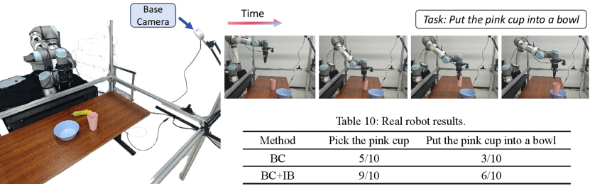
As shown in Figure 10, our real-world experiments involve a 6-DOF UR5 arm equipped with a Robotiq 2F-85 gripper and a RealSense L515 camera (base camera) for RGB image capture. We designed two simple tabletop manipulation tasks with manipulation skills:
-
•
Pick. The robot grips the pink cup on the table and lifts it up in the sky.
-
•
Pick and Place. The robot grips the pink cup on the table and places it in the bowl.
The demonstrations used for training both BC and BC+IB policies are collected using a 3D mouse, with 25 demonstrations recorded for pick tasks and 50 for more challenging pick-and-place tasks, utilizing only the base camera. We adopt VC-1 (Majumdar et al., 2023) as the baseline BC method, where pre-trained representations remain frozen during policy training, maintaining consistency with the simulation setup. To ensure a fair comparison, all methods are evaluated under identical initial conditions for each task.
The real-world robot experiments demonstrate that incorporating IB into BC significantly enhances task success rates. As shown in Table 10, BC+IB achieves a 9/10 success rate for picking the pink cup, compared to 5/10 for standard BC. Similarly, in the more complex task of placing the pink cup into the bowl, BC+IB outperforms BC with a success rate of 6/10 versus 3/10. This indicates that reducing redundancy in latent representations improves both grasping stability and overall task execution.
C.3 Extention to Few-shot Setting
We further evaluate the effectiveness of IB in a few-shot setting by conducting experiments with BC-VILT across multiple suites in LIBERO, as illustrated in Figure 11. The model is trained with only 10 demonstrations. The results consistently show that incorporating the IB improves success rates across all LIBERO suites, highlighting its efficacy in few-shot learning scenarios.
C.4 Experiments on LIBERO-Object of LIBERO
We observe that in the LIBERO-Object suite, the success rate does not consistently improve with an increasing number of demonstrations. Specifically, in the 10-shot setting, BC-VILT achieves a success rate of 56.17%, but in the full-shot setting, its performance drops to 43.00%. We hypothesize that this decline stems from inherent data distribution characteristics within the benchmark. In particular, we suspect that task-level imbalance in the dataset may contribute to overfitting.