2023
[2]\fnmJun \surYang
1]\orgnameZhejiang Sci-Tech University, \orgaddress\cityHangzhou, \countryChina 2]\orgnameJiaxing University, \orgaddress\cityJiaxing, \countryChina
Rethinking PRL: A Multiscale Progressively Residual Learning Network for Inverse Halftoning
Abstract
Image inverse halftoning is a classic image restoration task, aiming to recover continuous-tone images from halftone images with only bilevel pixels. Because the halftone images lose much of the original image content, inverse halftoning is a classic ill-problem. Although existing inverse halftoning algorithms achieve good performance, their results lose image details and features. Therefore, it is still a challenge to recover high-quality continuous-tone images. In this paper, we propose an end-to-end multiscale progressively residual learning network (MSPRL), which has a UNet architecture and takes multiscale input images. To make full use of different input image information, we design a shallow feature extraction module to capture similar features between images of different scales. We systematically study the performance of different methods and compare them with our proposed method. In addition, we employ different training strategies to optimize the model, which is important for optimizing the training process and improving performance. Extensive experiments demonstrate that our MSPRL model obtains considerable performance gains in detail restoration.
keywords:
Image inverse halftoning, error diffusion, multiscale progressively learning, deep learning.1 Introduction
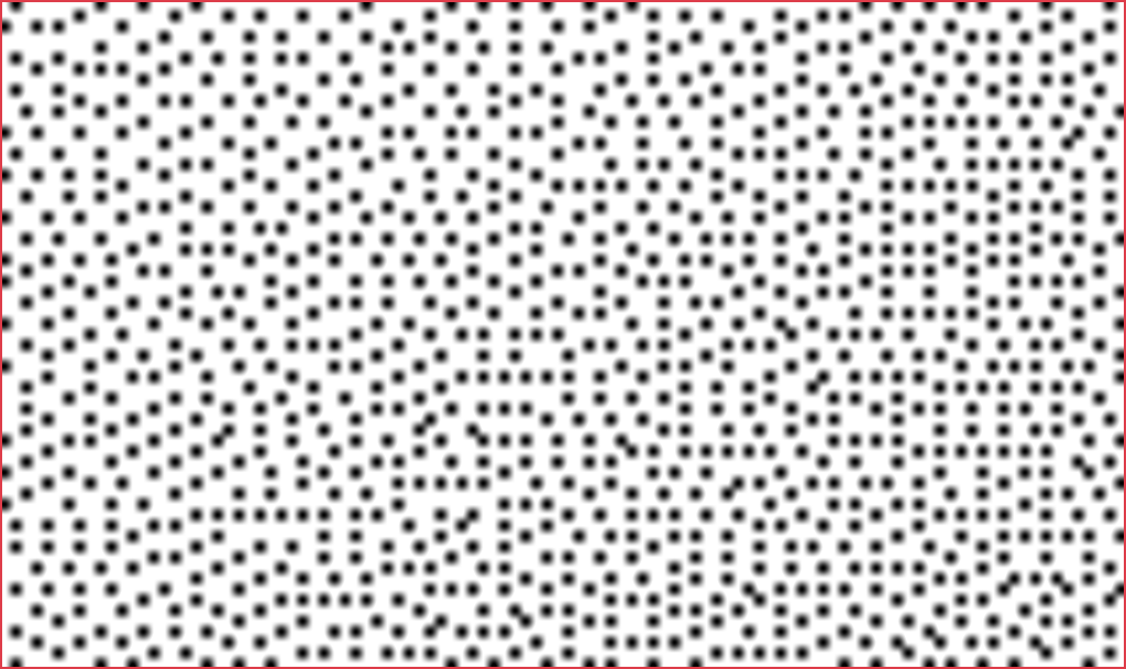
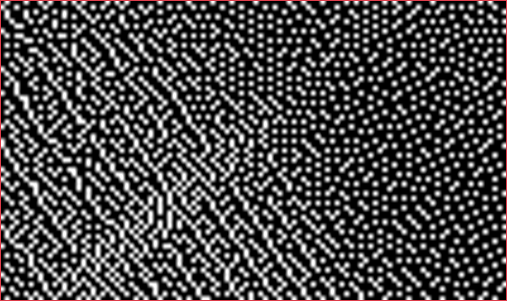
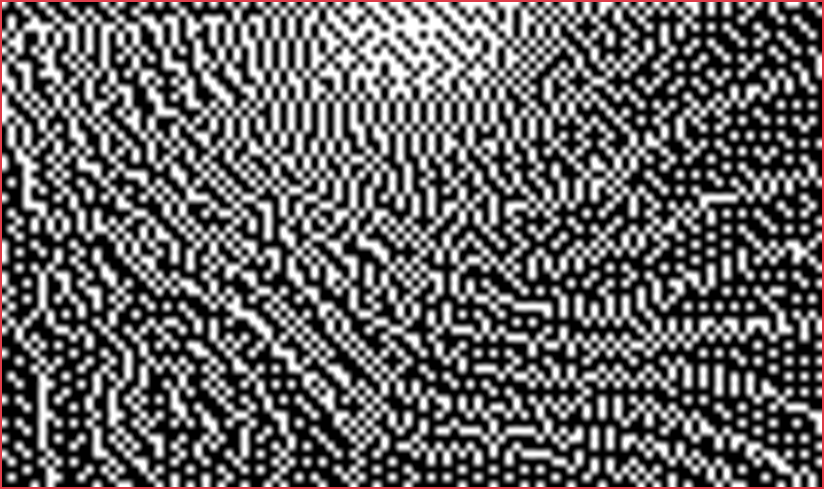
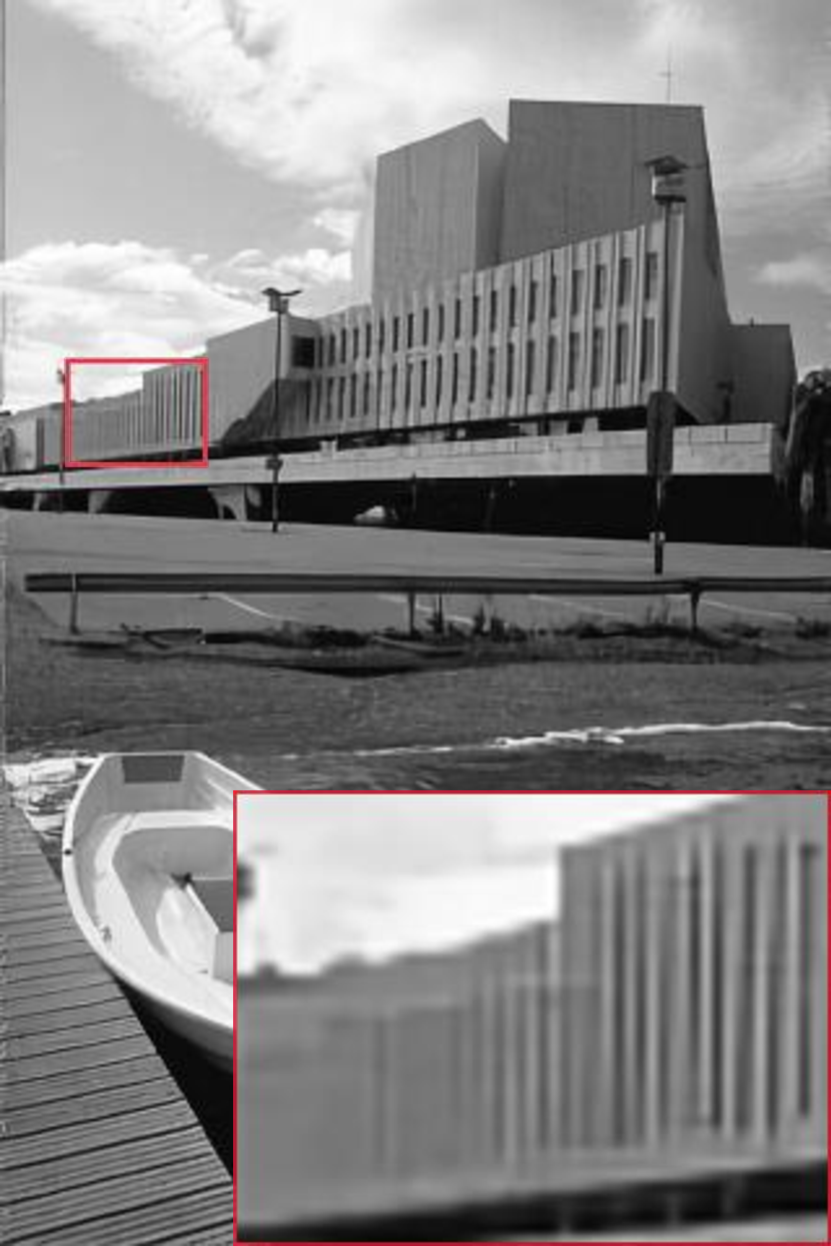
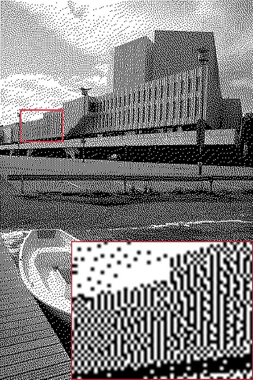
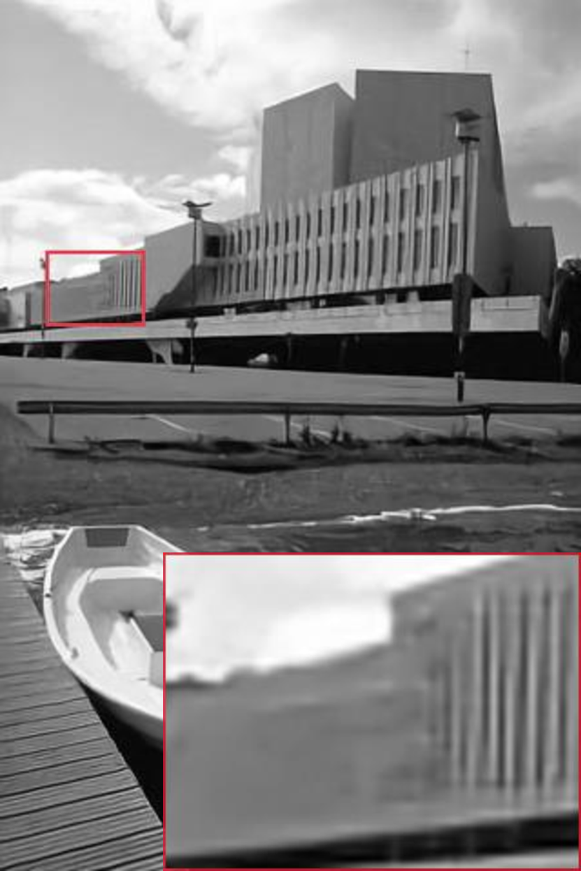
The halftoning method represents continuous-tone images with two levels of color, namely black and white, due to cost considerations and is commonly used in digital image printing, publishing and displaying applications (Mulligan and Ahumada Jr, 1992). There are various methods for halftoning algorithms, such as error diffusion, dot diffusion, ordered dithering and direct binary search (Floyd, 1976; Eschbach and Knox, 1991; Knuth, 1987; Bayer, 1973; Seldowitz et al, 1987). Because the halftone image has only two values, it can save considerable storage space and network transfer bandwidth compared to continuous-tone images. It is also a feasible and important image compression method. Fig. 1 illustrates an original grayscale image, corresponding to the halftone images and the inverse halftoning images.

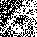
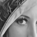
Image inverse halftoning is an image restoration task that reconstructs continuous-tone images with 255 or more levels from its corresponding halftone images. The purpose is to convert a binary image at into a continuous image in space, where and are the image height and width respectively. Because the halftone image loses many detailed features during the halftoning process, it is a challenging and ill-posed problem. In the past several decades numerous image inverse halftoning approaches have been explored to achieve good inverse halftoning performance (Kite et al, 2000; Analoui and Allebach, 1992; Mese and Vaidyanathan, 2001; Liu et al, 2010; Wong, 1995).
Owing to the success of deep convolutional neural networks (CNNs) in vision tasks, CNN-based image restoration methods have been extensively studied and have shown amazing performance. Several inverse halftoning methods based on deep learning have also achieved the significant advancements (Hou and Qiu, 2017; Xiao et al, 2017; Yuan et al, 2019; Xia and Wong, 2018). These methods mainly use the typical UNet architecture to build their CNN models. The UNet architecture is a multilevel design that aims to recover detailed features by extracting different information at multiple scales of the image. Therefore, it is widely used as a baseline in many vision models.
However, there is still a certain gap in detail restoration. Although most of the existing methods use the UNet architecture, they cannot effectively extract features at different image scales, because of which the quality of image reconstruction still has much room for improvement. Previous studies (Hou and Qiu, 2017; Xiao et al, 2017; Yuan et al, 2019) did not effectively extract image textures and features of multilayer downsampled images, and failed to restore high-quality continuous-tone images. In addition, Shao et al (2021) added an attention mechanism to enhance the detail extraction, but, despite the increased complexity of the model, there was no obvious performance improvement.
In this paper, we present a novel multiscale progressively learning network architecture that inspired by precious progressively learning UNet architectures (Zamir et al, 2022; Chen et al, 2022; Cho et al, 2021). Our model takes multiscale input images and uses a shallow feature extraction module to extract similar features from multiscale images. The encoder and decoder are composed of multiple residual block modules. Then, the feature fusion module fuses the output images of different stages of the encoder as the input images of the decoder, and finally outputs the continuous-tone images via progressively learning, which can ensure the efficiency of the model’s learning ability. We conduct experiments on the VOC2012 dataset, which is widely used in other vision tasks, such as image classification, object detection and instance segmentation. The main contributions of this paper are as follows.
1) Our MSPRL contains encoder and decoder stages. The encoder is mainly responsible for restoring image information and removing noise that affects image quality. The decoder aims to recover the texture details of different feature maps from the encoding stage, and outputs continuous-tone grayscale images. Meanwhile, we compare some common feature extraction blocks in the encoder and decoder.
2) We propose a computationally inexpensive shallow feature extraction module (SFE) to extract attention information between images to recover content feature representation and use a feature fusion module (FF) to fuse different stages of feature information.
3) Compared with other researchers who are keen on designing model architectures, we delve into the optimization of training strategies. Good training strategies for the performance improvement of the model are obvious and are used in our model training process, such as data augmentation methods and compound loss functions, which bring considerable improvements to model training and optimization.
2 Related Work
2.1 Conventional Inverse Halftoning
During the last decade, many approaches have been proposed for image inverse halftoning. Simple approaches use low-pass filtering to remove halftone noise (Wong, 1995; Catté et al, 1992). Although these methods can remove most of the halftone noise, they also remove high-frequency edge information. Thus, Kite et al (2000) proposed gradient-based spatially varying filtering for error diffused images to better recover high-frequency details of images. Unal and Çetin (2001), and Analoui and Allebach (1992) proposed projection onto the convex sets method (POCS) for inverse halftoning. In addition, some researchers used wavelet-based methods to separate halftoned image noises and then reconstruct the original image by wavelet shrinkage. Based on the Bayesian approach, Liu et al (2010) built a correlation map between adjacent points for inverse halftoning. Dictionary-based learning has also been widely and successfully applied to inverse halftoning (Zhang et al, 2018b). Son and Choo (2014) proposed an edge-oriented local learned dictionaries (LLD) method to enhance the edge details of the restored image. Considering computational efficiency, Mese and Guo further proposed a precomputed look-up table (LUT) (Mese and Vaidyanathan, 2001; Guo et al, 2013) to improve performance and utilize efficiency. Huang et al (2008) used a hybrid neural network method to process halftone and inverse halftoning images.
2.2 Deep Convolutional Neural Networks
Deep convolutional neural networks (CNNs) have become the dominant method for solving various image reconstruction problems and have achieved state-of-the-art performance on a wide variety of vision datasets. SRCNN (Dong et al, 2014) first introduced CNNs to the image super-resolution (SR) task, which focuses on reconstructing high-resolution (HR) details from corresponding low-resolution (LR) images, and obtains superior performance against previous conventional SR methods. ResNet (He et al, 2016) introduced an identity skip connection that alleviates the difficulty of model degradation in deep neural networks and allows networks to learn deeper feature representations. VDSR (Kim et al, 2016) achieved a good recovery effect using a residual learning architecture for super resolution. EDSR (Lim et al, 2017) built a very wide network using residual blocks. DnCNN (Zhang et al, 2017) used CNNs to remove the white Gaussian noise of images. MIMO-UNet (Cho et al, 2021), NAFNet (Chen et al, 2022) and Restormer (Zamir et al, 2022) presented the multi-input fusion UNet architecture to aggregate multiscale feature information for image deblurring and image deraining.
Image inverse halftoning is similar to many image restoration tasks. Thus, Hou and Qiu (2017), and Xiao et al (2017) applied CNNs to inverse halftoning by building a UNet network as the restoration network. Xia and Wong (2018) proposed a progressively residual learning network (PRL) including two main stages: the content aggregation stage, which restores the content map, and the detail enhancement stage, which restores the extract texture and details. Yuan et al (2019) proposed gradient-guided residual learning CNNs (GGRL) for inverse halftoning. The same subnetworks are used to learn gradient maps of different Sobel orientations from the input halftone image, and a coarse map is output that is used to restore the continuous-tone images. Shao et al (2021) presented an attention model for inverse halftoning by using residual channel attention blocks (RCAB) (Zhang et al, 2018a). Xia et al (2021) and Yen et al (2021) combined inverse halftoning with image colorization methods to recover color continuous-tone images with better visual quality from corresponding halftone grayscale images.
2.3 The importance of training strategies
Better training strategies can increase the performance of a model and effectively decrease the training time (Goyal et al, 2017; He et al, 2019; Qian et al, 2022; Lin et al, 2022). Data augmentation is one of the most important strategies to boost the performance of a neural network (Cubuk et al, 2020). It can provide more learning samples and improve model generalization through various random changes for training images. Many researchers use cosine annealing (Loshchilov and Hutter, 2016) decay to boost performance. Furthermore, the warm-up method (Goyal et al, 2017; He et al, 2019) is used to alleviate the instability of the model in the early training stage. In many vision tasks, removing batch normalization (BN) layers can increase performance and reduce computational complexity such as SR and deblurring (Lim et al, 2017; Wang et al, 2018). Zhao et al (2016) showed that L1 loss has a better convergence effect and image perceptual quality than L2 loss. In this paper, we adopt suitable training strategies for our inverse halftoning task to improve the visual quality of restored continuous-tone images.
3 Methodology
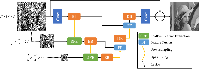
In this section, we first introduce our MSPRL model based on the UNet architecture and propose the shallow feature extraction module (SFE) in Sec. 3.1. The overall architecture of MSPRL is shown in Fig. 2. Then we describe our loss function in Sec. 3.2. Last, we use an overall different training strategy compared with PRL in Sec. 3.3.
3.1 model architecture
As shown in Fig. 2, given a halftone input image , the goal of our method is to restore the clear and continuous-tone grayscale image by progressively learning. Our model is mainly divided into two stages: the left encoder (EC) stage and the right decoder (DC) stage, and three levels from top to bottom.
Overall Pipeline. In the encoder stage, we first use a 33 convolution layer to obtain a low-level feature map F, where denotes the spatial dimension, is the number of feature map channels that we set to 48, represents the level and EB represents encoder block that consist of 8 residual blocks (RBs). Then, F passes through an encoder EBk which transforms it into deep feature maps at level 1. EBk obtains an output EB by downsampling, where the number of channels is doubled and the image size is halved. For the downsampling and upsampling modules, we apply pixel-unshuffle and pixel-shuffle operations respectively. To extract the similar information of multiscale images, we use the shallow feature extraction module (SFE) to exploit the attention features of EB and X in the second and third levels, respectively, and output the fusion attention feature maps of SFEk, where uses linear interpolation downsampling from the corresponding -1 level of the input image . Then SFEk passes through EB to obtain deep features. The left encoding stage process is defined as:
| (1) |
where is the input image, represents a 33 convolutional layer, and EBk and SFEk represent the outputs of the level EB and SFE respectively.
In MSPRL, the decoder takes the encoder features EB as input and progressively recovers the continuous-tone representations. First, the feature fusion module (FF) aggregates the feature maps of different encoder stages EBk and EB and outputs the aggregated features FFk. Then, we use the decoder block (DB) DBk to reconstruct the image details, where DB is also composed of 8 residual blocks (RBs). Through a series of decoding and reconstruction, we obtain F. Finally, we apply a 33 convolution and residual connection to obtain the final continuous-tone image . The overall process is progressively learning. The right decoding stage process is defined as:
| (2) |
| (3) |
where and are the input and output images, respectively, represents a 33 convolutional layer, and DBk and FFk represent the outputs of the DB and FF respectively, and = 1,2 in Eq. 2.
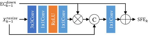
Shallow Feature Extraction and Feature Fusion. Inspired by the shallow convolutional module (SCM) in MIMO-UNet (Cho et al, 2021), our shallow feature extraction module (SFE) is shown in Fig. 3LABEL:sub@fig:3_1. The passes through a 33 convolutional layer and two stacks of 11 point-wise convolution to output a low-level feature map Conv. Then, we use element-wise multiplication to obtain attention features between the previous Conv and EB. A 11 point-wise convolution is used to aggregate the attention features of previous and EB, which are shown in Fig. 3LABEL:sub@fig:3_2. The SFE is formulated as:
| (4) |
| (5) |
where = 2,3 represents the level, , and represent multiple stacked convolutional layers, a 11 convolutional layer and element-wise multiplication respectively.
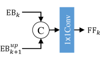
For the feature fusion module (FF), the FF aggregates the feature maps of EBk and EB and is formulated as:
| (6) |
where = 1,2 represents level and represents a 11 convolutional layer.
Downsampling and Upsampling. We use PixelShuffle as the upsampling and downsampling operation. Compared with convolution upsampling and downsampling, PixelShuffle can obtain better visual quality (Shi et al, 2016).
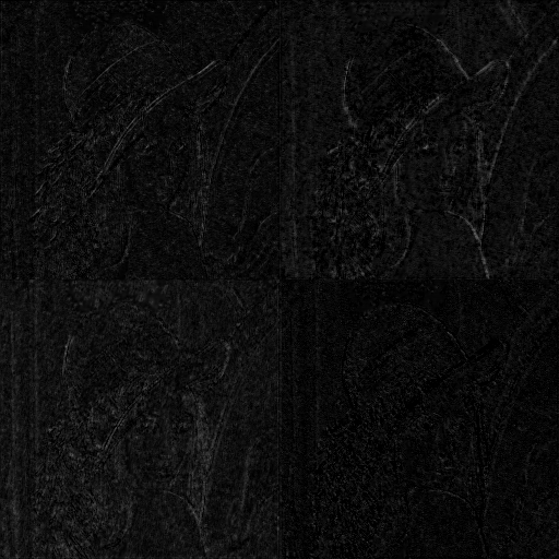
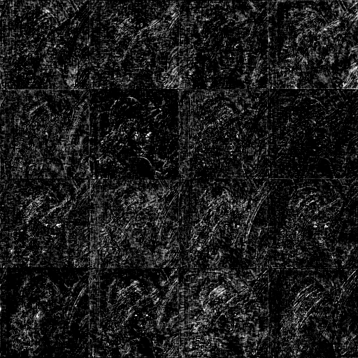
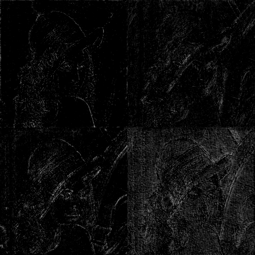
Progressively Learning. Progressively learning allows the network to learn local and global features, which makes full use of semantic information of different scale images. In addition, it can also greatly reduce the convolution operation time under the small image patches. The feature maps of different stages are shown in Fig. 4.
3.2 Loss Function
Although L1 loss, MSE loss and perceptual loss are used in PRL, we experimentally found that perceptual loss is added with a very large penalty coefficient, which has little effect on model convergence, and that MSE loss has a smooth ing effect. In this paper, we only use L1 loss as follows:
| (7) |
where is the pixel-wise loss that evaluates the L1 distance between recovered image and the ground-truth gray image . Some studies have shown that composite loss functions can improve performance. Inspired by (Cho et al, 2021), we add the fast Fourier transform (FFT) (Cochran et al, 1967) loss function to strengthen the high-frequency extraction as follows:
| (8) |
where FFT represents the fast Fourier transform that transfers the image signal to the frequency domain and uses L1 loss to evaluate the distance between recovered image and the ground-truth gray image . The final loss function for training our model is as follows:
| (9) |
where we set = 0.1 in experiment.
3.3 Training strategies
We first show the different training strategy comparisons in Tab. 1. Then we illustrate the strategies that differ from PRL.
Data augmentation. We found that other researchers use the resize operation to scale the images to 256256. However, this resizing operation results in the loss of much of detail and texture information of the original image. During our training period, we use random cropping on the training data so that the model can learn image information of different regions. Data augmentation enables the model to learn richer feature representations and improves model generalization.
Bigger batch-size. The original PRL uses a minimum batch-size of 1. A smaller batch size will make the model training unstable and affect the convergence speed. We use the most commonly used batch-size 16.
Optimizer and Schedule. Unlike PRL, we utilize the AdamW optimizer (Loshchilov and Hutter, 2017) instead of Adam (Kingma and Ba, 2014) and optimizer momentum with (). For the learning rate decreasing strategy, we use the cosine annealing decay schedule (Loshchilov and Hutter, 2016) instead of linear decay.
4 Experiments
In this section, we first describe the datasets, evaluation metrics and training details. We then show the impact of different training strategies in the same baseline PRL. We demonstrate the performance of the different models later.
4.1 Datasets and Implementation Details
Datasets and Metrics. Following the PRL, we use the VOC2012111http://host.robots.ox.ac.uk/pascal/VOC/. dataset (Everingham et al, 2015), which includes over 17000 images. We randomly select 13841 images for training and 3000 nonoverlapping images for validation, where excluding images patch size smaller than 256256. We evaluate the model on the Place365222http://places2.csail.mit.edu/. small test dataset (Zhou et al, 2017), In addition, some classic images, such as Lena, Barbara and Baboon, and the Kodak333http://r0k.us/graphics/kodak/. dataset are added to the test dataset. We also test five standard SR benchmark datasets including Set5 (Bevilacqua et al, 2012), Set14 (Zeyde et al, 2010), BSD100 (Martin et al, 2001), Urban100 (Huang et al, 2015) and Manga109 (Matsui et al, 2017), where some images are properly cropped to fit the original PRL (Xia and Wong, 2018) model. In the experiment, the halftone images for all datasets are generated by the Floyd Steinberg error diffusion algorithm (Floyd, 1976). For the evaluation metrics, the peak signal to noise ratio (PSNR), and the structural similarity metric (SSIM) are used in all experiments. Our code and pre-trained models are available at https://github.com/FeiyuLi-cs/MSPRL.
| Training config | PRL | MSPRL |
|---|---|---|
| System implement | TensorFlow | Pytorch |
| Dataset size | 13K | 13K |
| Data augment | ✗ | ✓ |
| Batch size | 1 | 16 |
| Image size | 256 | 128 |
| Epochs | 150 | 347 |
| Total iterations | 1950K | 300K |
| Channel dimension | 64 | 48 |
| Optimizer | Adam | AdamW |
| Optimizer momentum | ||
| Learning rate decay | ||
| Learning rate schedule | Linearly decay | Cosine decay |
| Loss function | L1+MSE+Perceptual Loss | L1+FFT Loss |
| \botrule |
Training detail. In the training process, the batch-size is set to 16, and then the sampled images are randomly cropped to 128128. For data augmentation, each image patch is horizontally flipped with a probability of 0.5. We use iterations instead of epochs to represent the training length. The model is trained by the AdamW optimizer (Loshchilov and Hutter, 2017) () for 300K iterations. The initial learning rate is set to 0.0002, which gradually decays to with cosine annealing (Loshchilov and Hutter, 2016). The model training time is approximately 18 hours and runs on one Nvidia RTX 3090 GPU.
4.2 Ablation study
In this section, we conduct experiments to show the effects of different modules, activation functions and feature blocks with our method. Our MSPRL model employs 8 residual blocks for each encoder and decoder. First, we evaluate the effectiveness of MSPRL without SFE and FF. The experimental results are shown in Tab. 2. The FF improves PSNR by 0.02 dB compared with SFE in the Kodak datasets, and the performance gain is further increased to 0.05 dB when we combine FF with SFE. The results show that aggregating feature maps from different encoders is more important than computing attention feature maps for our model learning.
Many vision networks adopt ReLU (Nair and Hinton, 2010) or LeakyReLU (Maas et al, 2013) as the activation function. In recent years, GELU (Hendrycks and Gimpel, 2016) has gradually become the first choice. Therefore, we test three activation functions to explore the best performance for our method. The experimental results are shown in Tab. 3. The results show the effect of different activation functions on model performance. ReLU performs better overall on multiple datasets; the results of LeakyReLU and GELU are close to ReLU but add some training time. Thus, we choose ReLU as the activation function in our model.
| SFE | FF | Place365 | Kodak | ||
|---|---|---|---|---|---|
| PSNR | SSIM | PSNR | SSIM | ||
| ✓ | 30.76 | 0.9019 | 31.84 | 0.8897 | |
| ✓ | 30.76 | 0.9019 | 31.86 | 0.8897 | |
| ✓ | ✓ | 30.77 | 0.9020 | 31.89 | 0.8898 |
| \botrule | |||||
| Method | Place365 | Kodak | ||
| PSNR | SSIM | PSNR | SSIM | |
| ReLU | 30.77 | 0.9020 | 31.89 | 0.8898 |
| LeakyReLU | 30.76 | 0.9015 | 31.87 | 0.8894 |
| GELU | 30.76 | 0.9017 | 31.85 | 0.8896 |
| \botrule | ||||
Besides, we also compared three common feature blocks: residual block (RB) (He et al, 2016), residual channel attention block (RCAB) (Zhang et al, 2018a) and residual-in-residual dense block (RRDB) (Wang et al, 2018) to explore the performance of encoder and decoder of MSPRL. Both RCAB and RRDB will increase the computational complexity, and RRDB will greatly increase the model parameters, while RB can maintain model performance between low computational complexity and parameters. Their parameters and performance comparisons are shown in Tab. 4.
| Method | Amounts | Total parameters | Place365 | Kodak |
|---|---|---|---|---|
| RB | 8 | 9681505 | 30.77 | 31.89 |
| RCAB | 8 | 9745489 | 30.79 | 31.85 |
| RRDB | 2 | 22082593 | 30.80 | 31.90 |
| \botrule |
4.3 Impact of Training Strategies
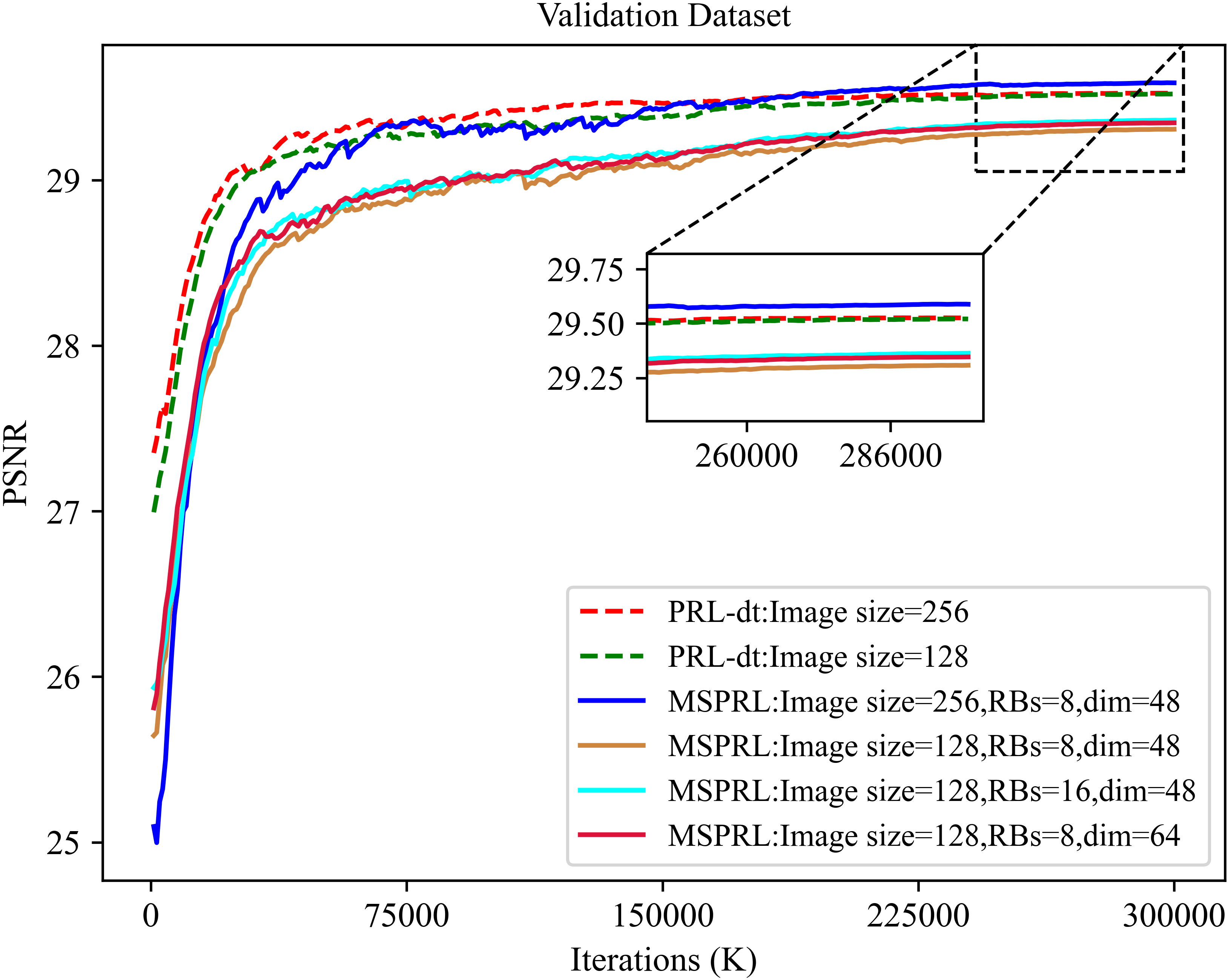
To explore the impact of training strategies, we conduct multiple experiments with different image sizes and loss functions using PRL and MSPRL models, respectively. We use the original PRL baseline and only use our different training strategies as shown in Tab. 1. The average improvement is approximately 1.5 dB in all test datasets, and is named PRL-dt. For image size, we found that the training time sharply decreased by approximately 70% when using images smaller than 128 pixels and that the performance was comparable to larger images of size 256. We assert that this phenomenon is due to data augmentation, random sampling and more iterations, which make the model learn as much feature information as from large images on small image sizes. For different loss functions, we minimize the fast Fourier transform loss in the frequency domain, so that the model can be further optimized and improved in image details compared to only using a single L1 loss function. The experimental results are shown in Tab. 6. Meanwhile, we also test the performance of our MSPRL with different numbers of channels and residual blocks in Tab. 5. The validation PSNR curves of the model under these different settings are shown in Fig. 5.
| Channels | RBs | Place365 | Kodak | ||
|---|---|---|---|---|---|
| PSNR | SSIM | PSNR | SSIM | ||
| 48 | 8 | 30.77 | 0.9020 | 31.89 | 0.8898 |
| 64 | 8 | 30.77 | 0.9022 | 31.89 | 0.8900 |
| 48 | 16 | 30.80 | 0.9025 | 31.93 | 0.8904 |
| \botrule | |||||
| Model | Image size | Training time | Place365 | Kodak |
| PRL | 256256 | - | 29.23 | 30.28 |
| PRL-dt | 256256 | 2 Days | 30.65 | 31.72 |
| 128128 | 17 Hours | 30.65 | 31.71 | |
| MSPRL(L1) | 128128 | 18 Hours | 30.75 | 31.82 |
| MSPRL | 256256 | 2.2 Days | 30.76 | 31.87 |
| 128128 | 18 Hours | 30.77 | 31.89 | |
| \botrule |
| Model | Place365 | Kodak | Set5 | Set14 | BSD100 | Urban100 | Manga109 | |||||||
|---|---|---|---|---|---|---|---|---|---|---|---|---|---|---|
| PSNR | SSIM | PSNR | SSIM | PSNR | SSIM | PSNR | SSIM | PSNR | SSIM | PSNR | SSIM | PSNR | SSIM | |
| DnCNN (Zhang et al, 2017) | 30.31 | 0.8913 | 31.24 | 0.8759 | 33.26 | 0.9192 | 30.76 | 0.8812 | 29.72 | 0.8600 | 29.81 | 0.9031 | 33.44 | 0.9427 |
| VDSR (Kim et al, 2016) | 30.15 | 0.8868 | 30.97 | 0.8718 | 32.92 | 0.9134 | 30.44 | 0.8758 | 29.53 | 0.8555 | 29.34 | 0.8964 | 32.87 | 0.9391 |
| EDSR (Lim et al, 2017) | 30.48 | 0.8960 | 31.48 | 0.8830 | 33.42 | 0.9219 | 30.95 | 0.8857 | 29.86 | 0.8652 | 30.22 | 0.9106 | 33.90 | 0.9466 |
| PRL (Xia and Wong, 2018) | 29.23 | 0.8840 | 30.28 | 0.8722 | 32.06 | 0.9103 | 29.97 | 0.8746 | 28.99 | 0.8525 | 29.39 | 0.9017 | 32.55 | 0.9365 |
| GGRL (Yuan et al, 2019) | 30.46 | 0.8960 | 31.44 | 0.8830 | - | - | - | - | 29.85 | 0.8654 | - | - | - | - |
| MIMOUNet (Cho et al, 2021) | 30.56 | 0.8977 | 31.55 | 0.8855 | 33.54 | 0.9235 | 31.07 | 0.8883 | 29.91 | 0.8674 | 30.41 | 0.9140 | 34.21 | 0.9488 |
| PRL-dt (ours) | 30.65 | 0.9000 | 31.71 | 0.8875 | 33.70 | 0.9254 | 31.25 | 0.8904 | 30.01 | 0.8691 | 30.71 | 0.9183 | 34.50 | 0.9502 |
| MSPRL (ours) | 30.77 | 0.9020 | 31.89 | 0.8898 | 33.81 | 0.9264 | 31.40 | 0.8925 | 30.09 | 0.8708 | 31.10 | 0.9226 | 34.85 | 0.9518 |
| \botrule | ||||||||||||||
4.4 Performance comparison
We compare MSPRL with other inverse halftoning methods and CNN models of relevant vision tasks, such as DnCNN (Zhang et al, 2017), VDSR (Kim et al, 2016) and EDSR (Lim et al, 2017). The single baseline model in EDSR, which contains 16 residual blocks with 64 convolution kernel channels, is used in our task. We remove data pre/postprocessing and upscaling layers. For GGRL (Yuan et al, 2019), the public pretrained model is not available and their training dataset size is 8 times our dataset. Therefore, we only use the GGRL model in our training process, leading to some gaps in its performance compared to the original paper. In order to distinguish similar models, we also test MIMOUNet (Cho et al, 2021). For a fair comparison, these methods employ our training strategies. Because DnCNN, VDSR and EDSR adopt our training strategy, their results are higher than the values of the corresponding models trained in (Xia and Wong, 2018). The performance comparison is demonstrated in Tab. 7. The experimental results show that our MSPRL obtains the best performance on multiple datasets by 0.3 dB gain. Especially on the Urban100 dataset, MSPRL is 0.69 dB higher than MIMOUNet, meanwhile, other models outperform the original PRL due to our training strategies. We also changed the training strategy of PRL, named PRL-dt, and its model performance greatly improved compared with original PRL. The average PSNR on multiple datasets improved by approximately 1.5 dB only by changing the training strategy. Finally, MSPRL also outperforms PRL-dt on all datasets.
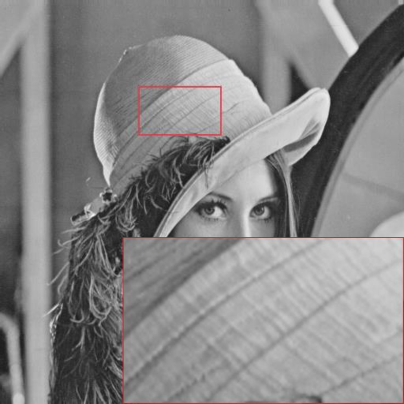
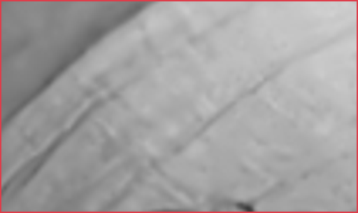


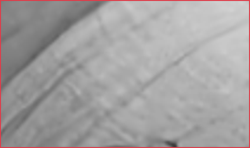


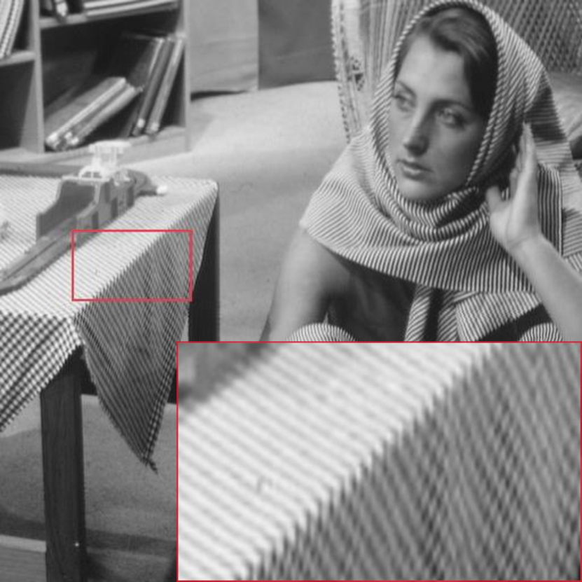
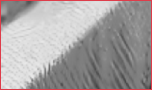


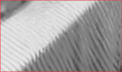
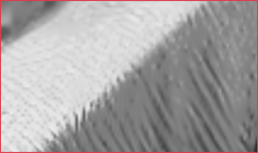

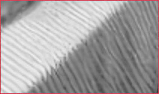

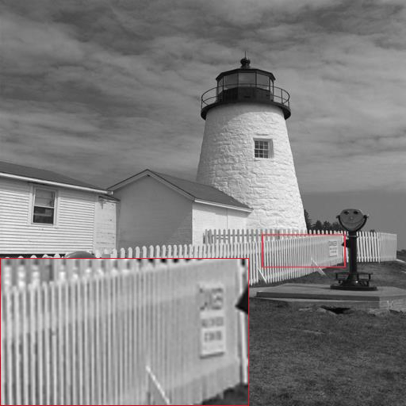
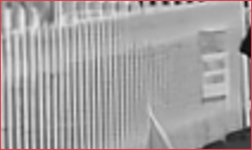
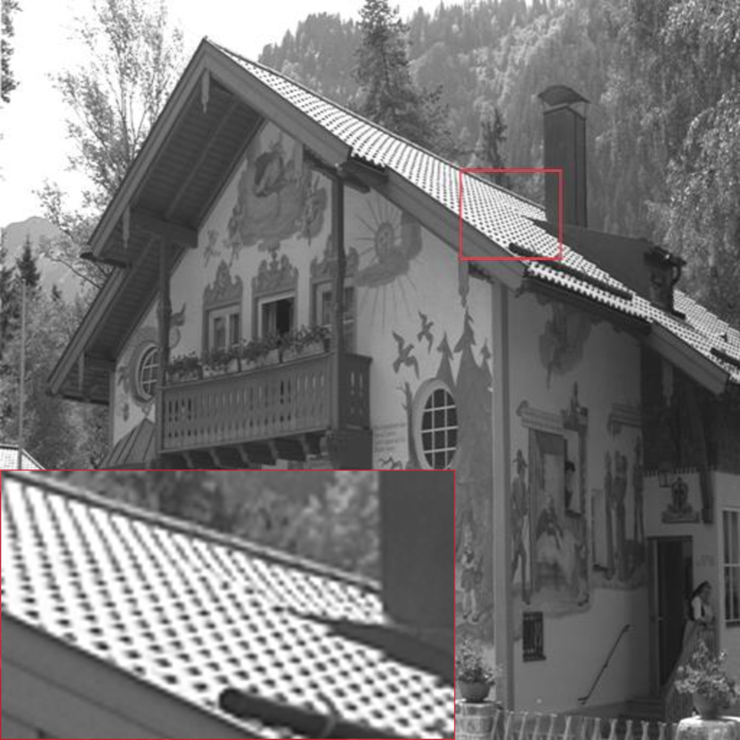
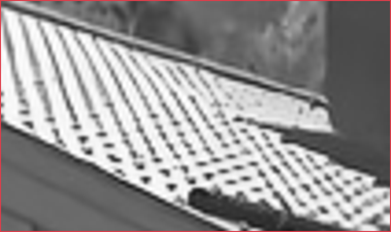
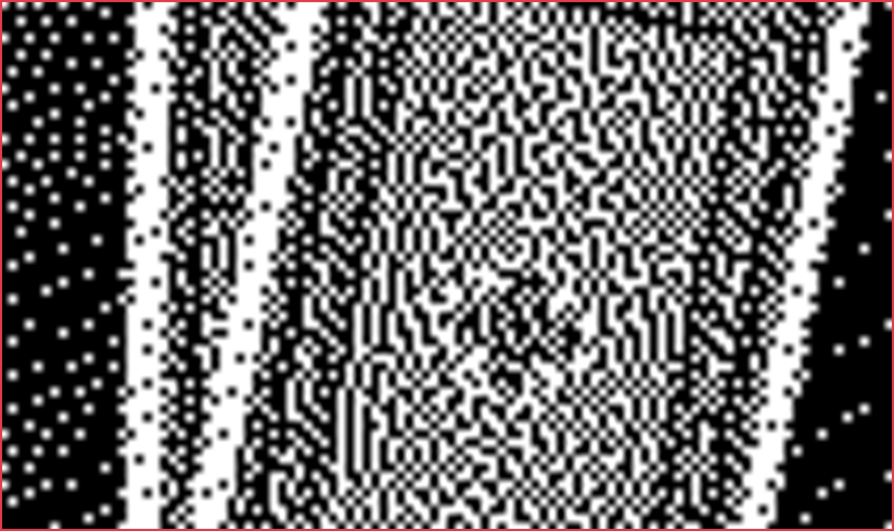
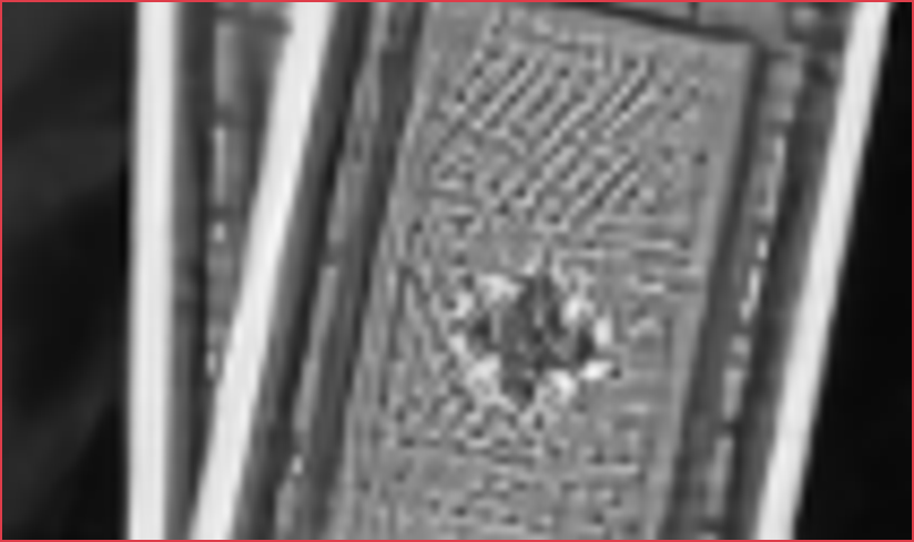
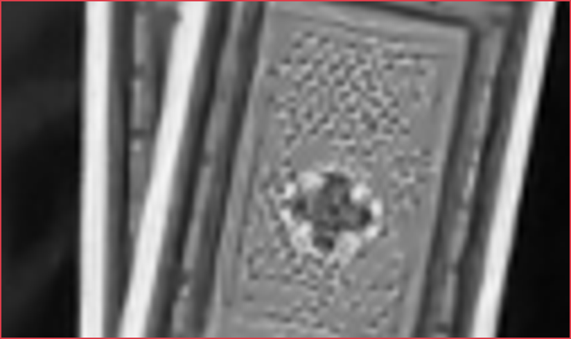
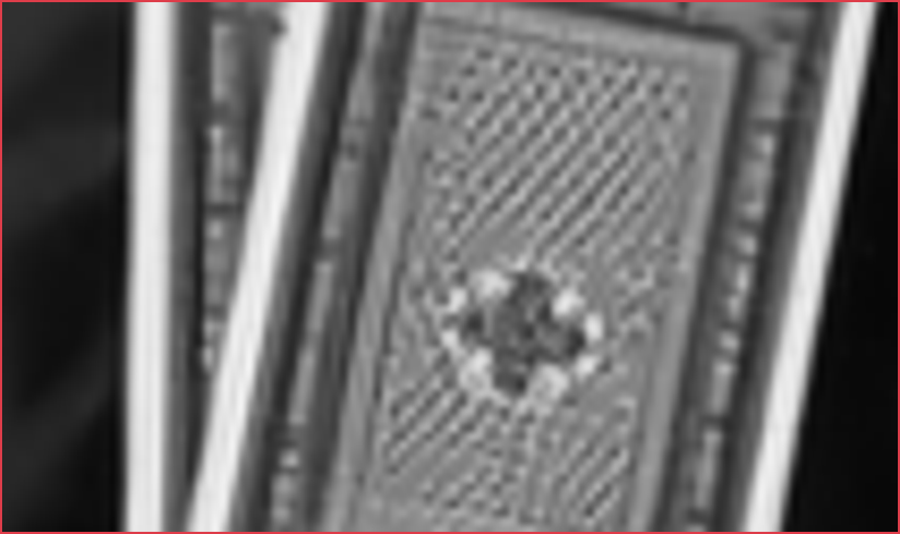
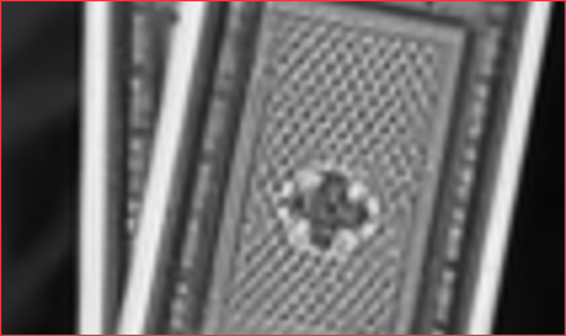
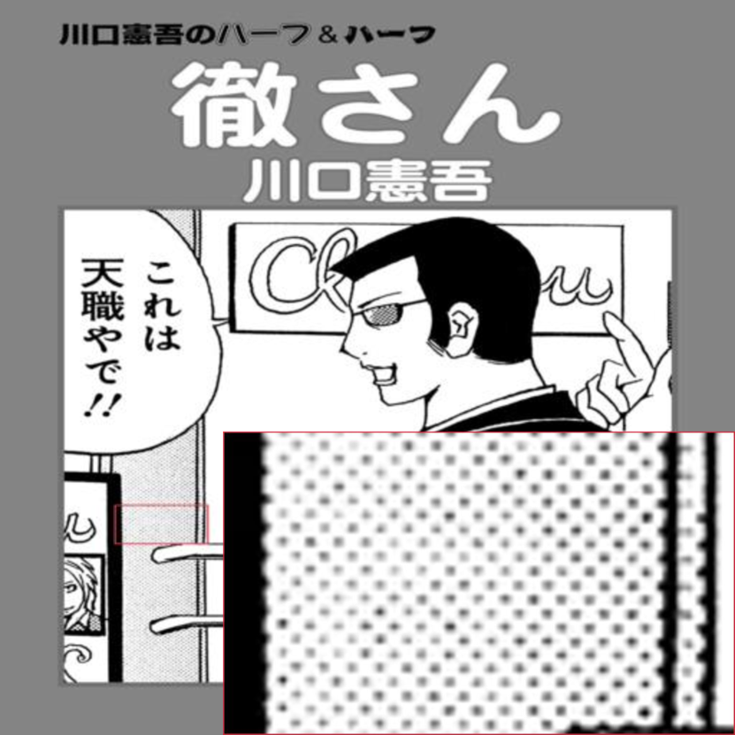
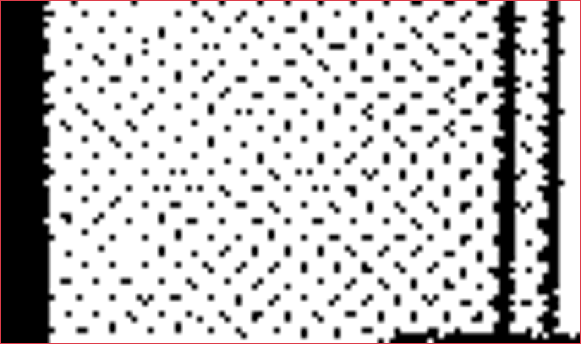
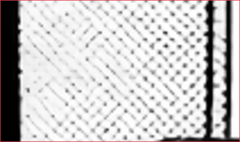
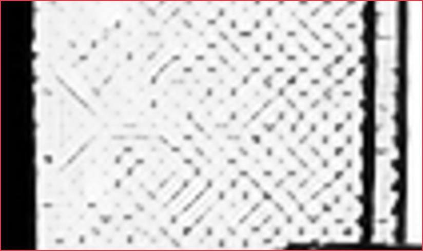
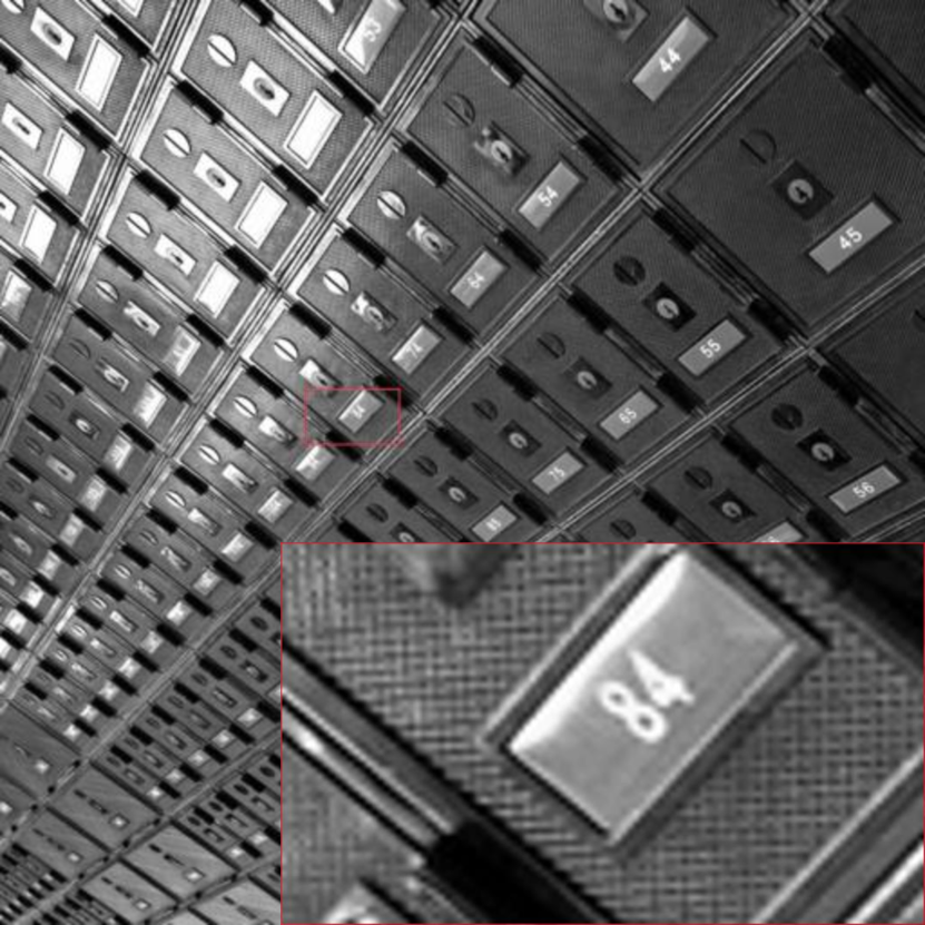
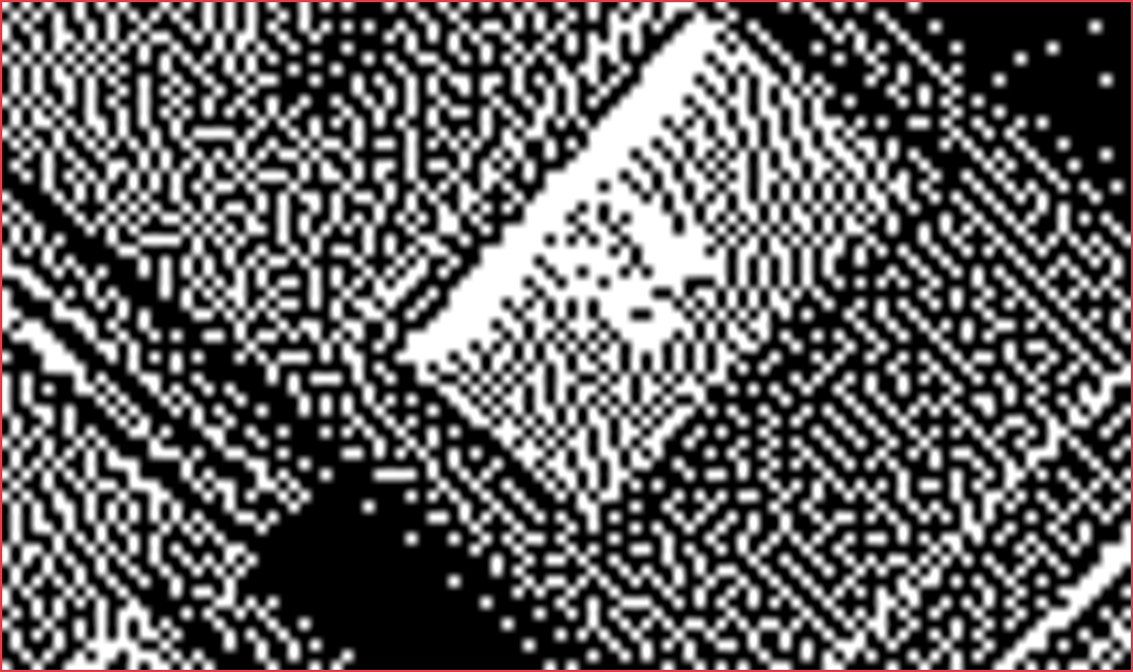
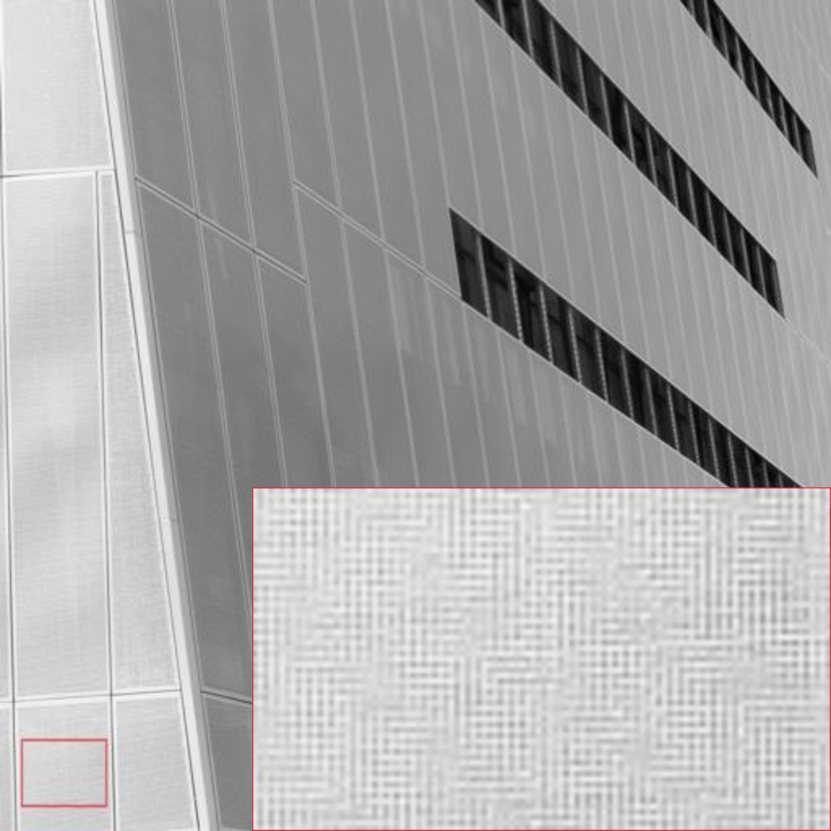
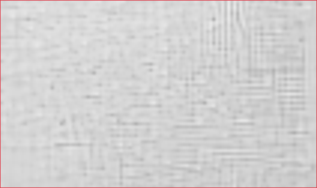
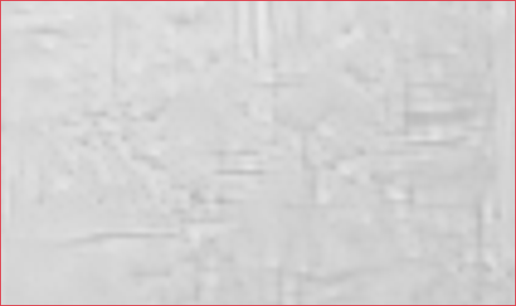
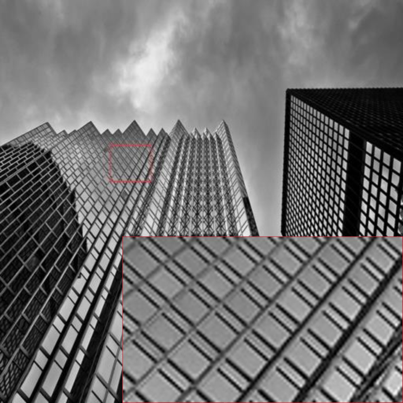
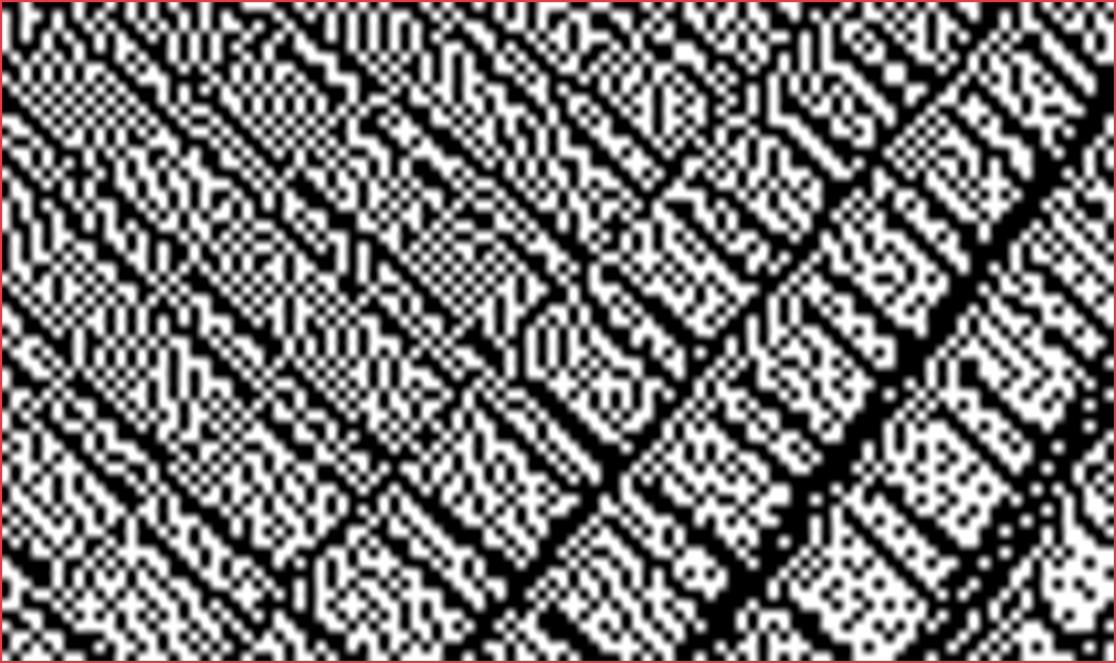
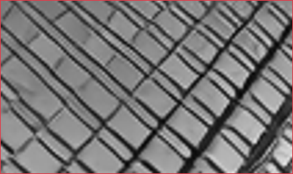
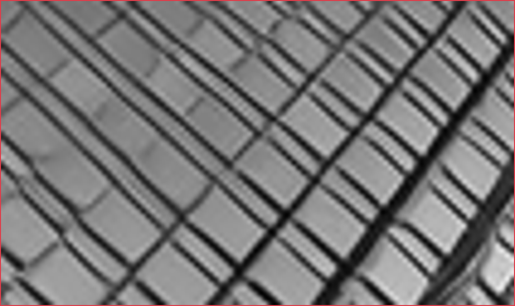
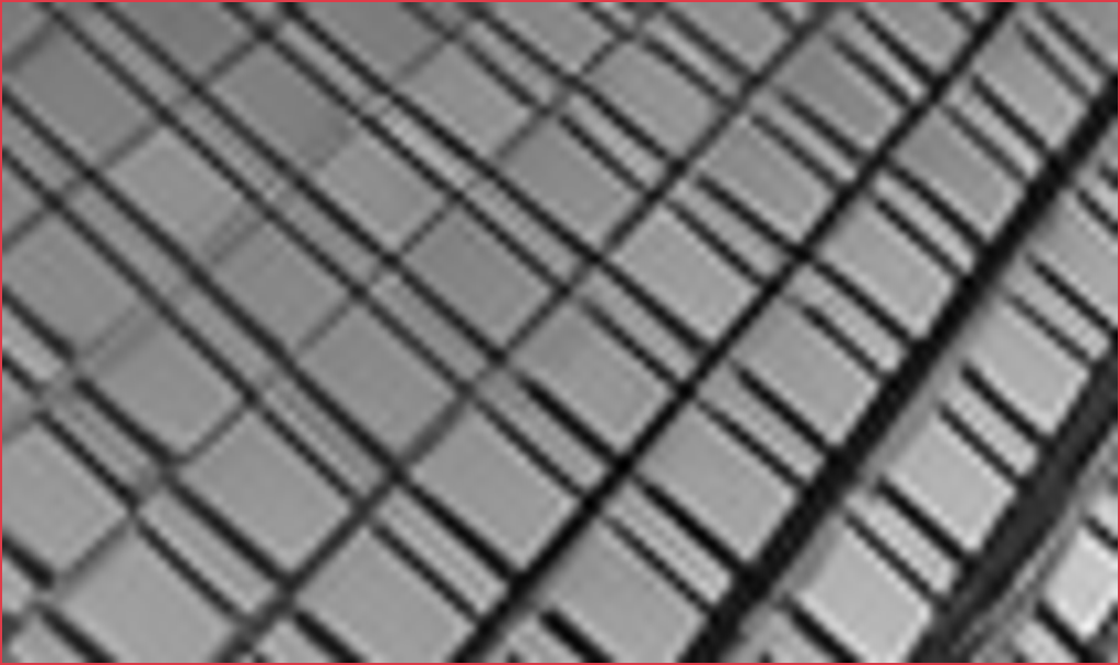
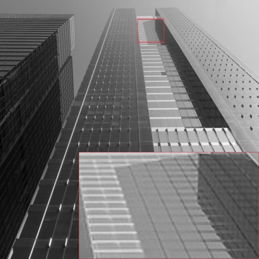
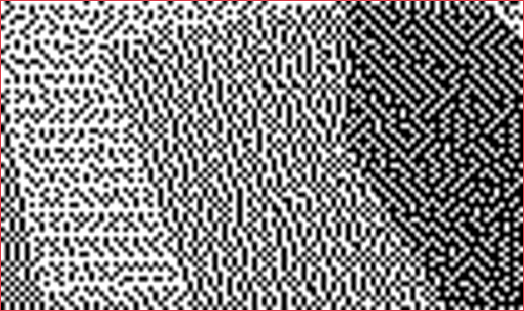
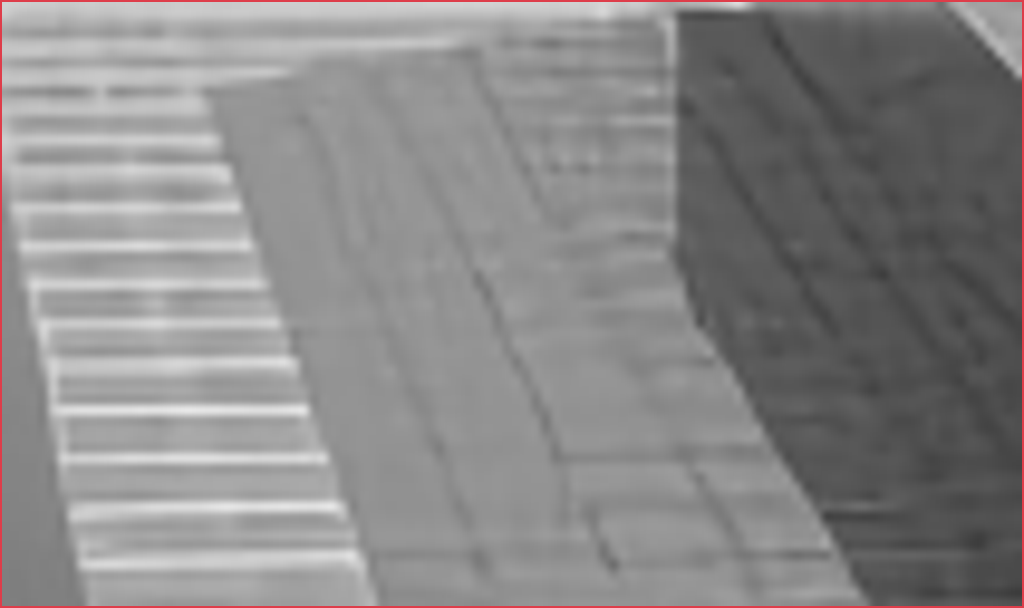
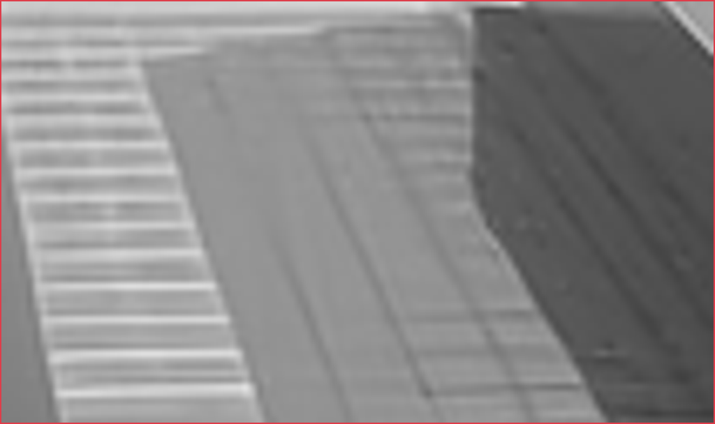
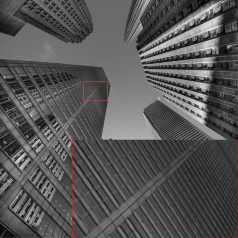
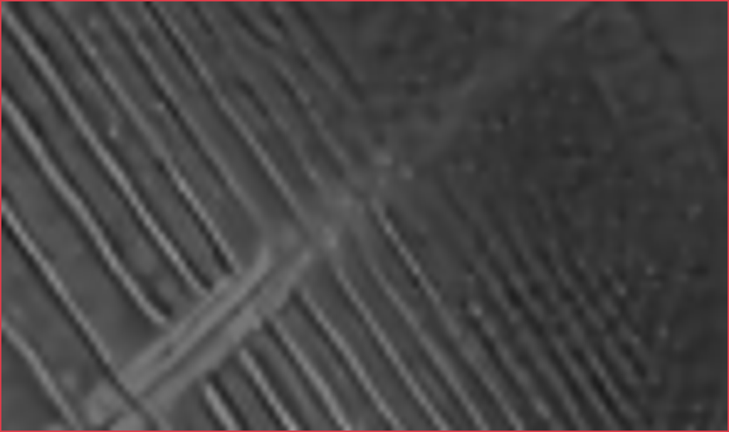
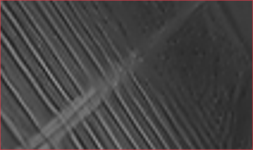
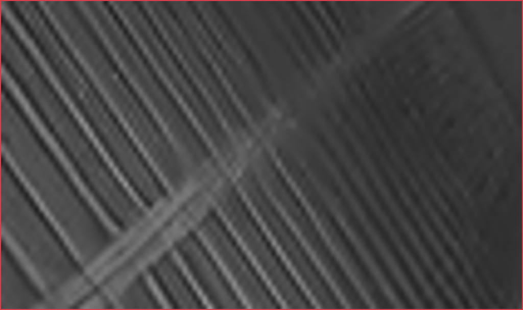
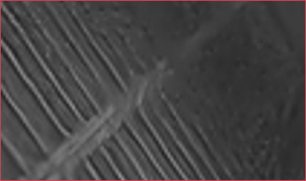
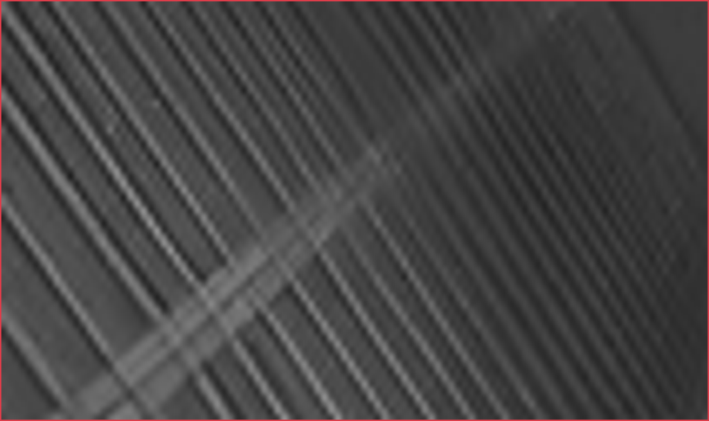
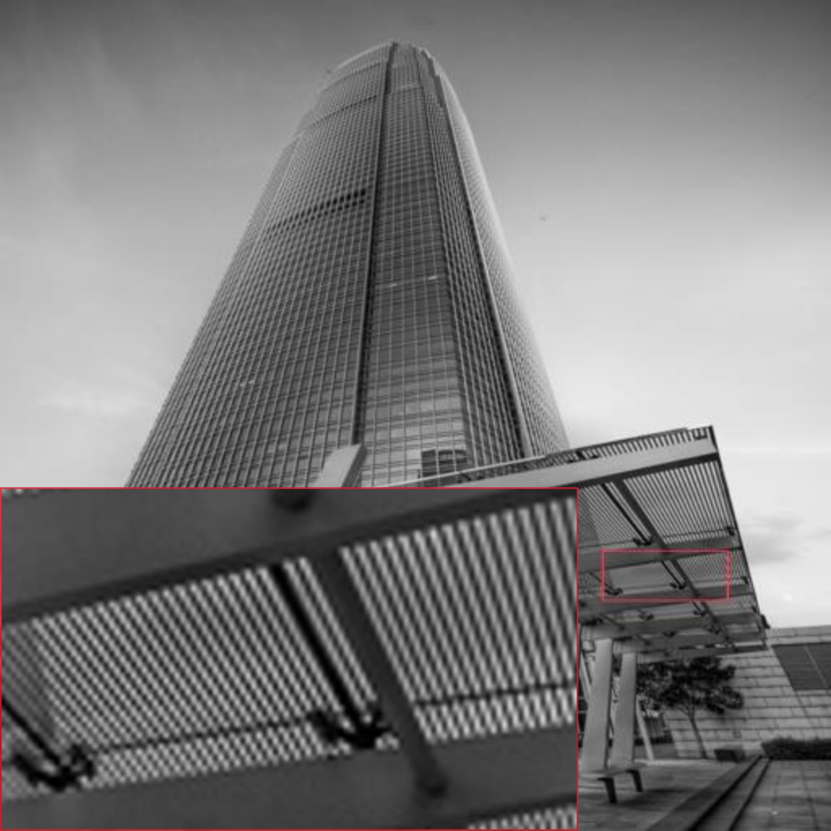
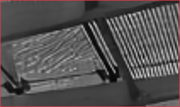
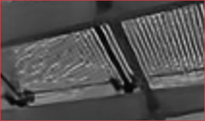
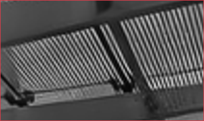
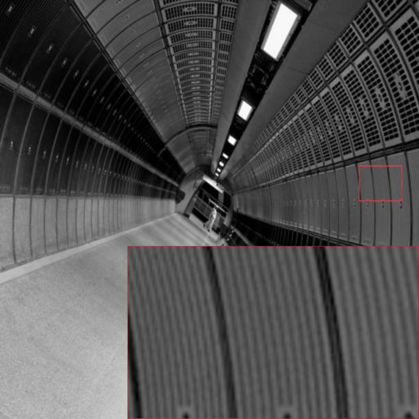
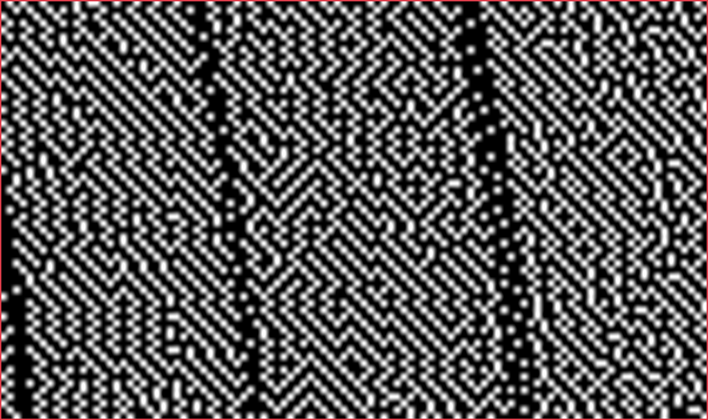
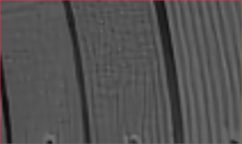
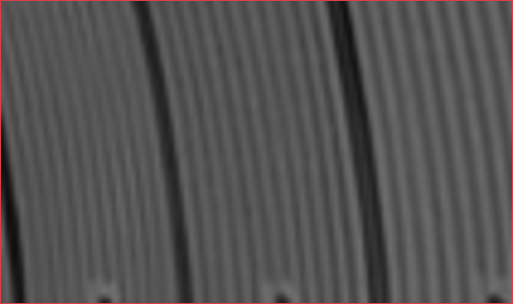
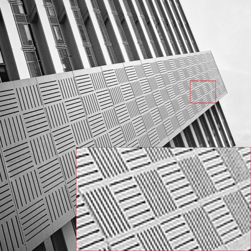
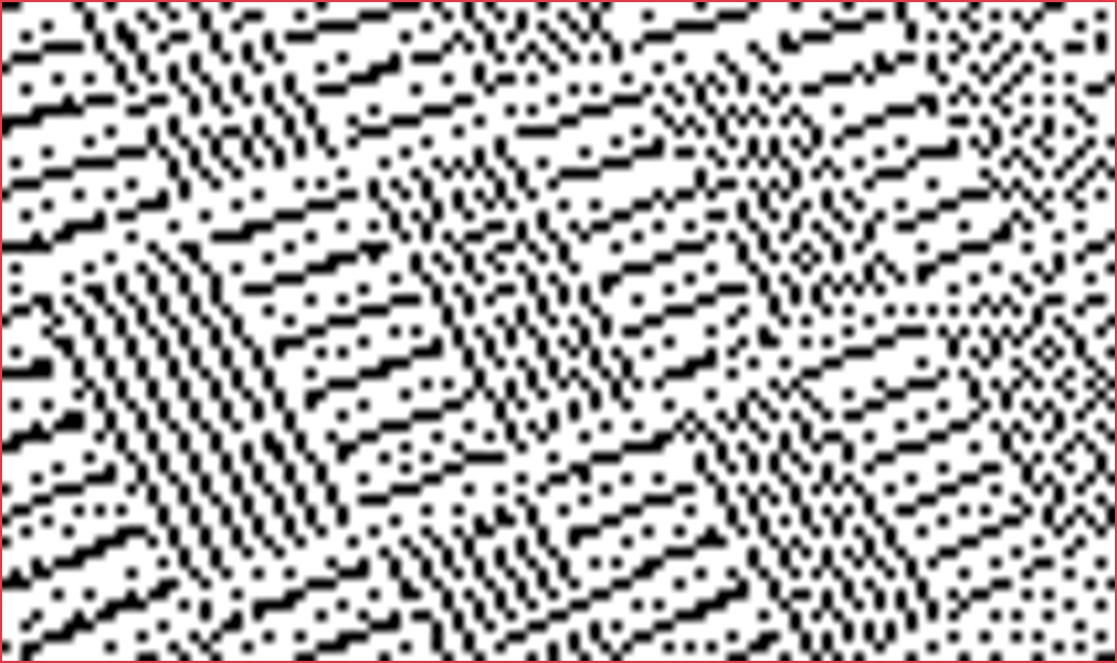
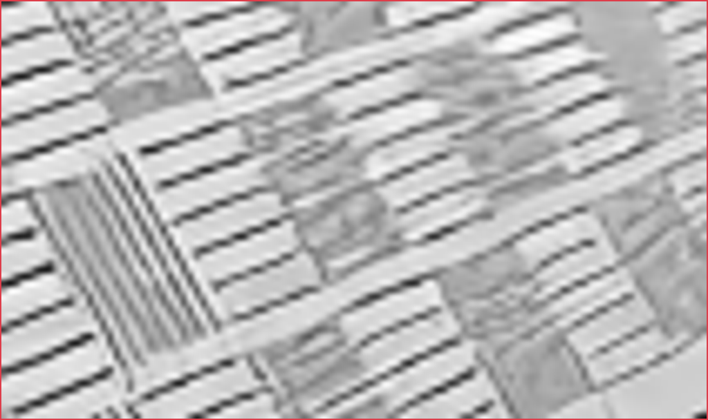
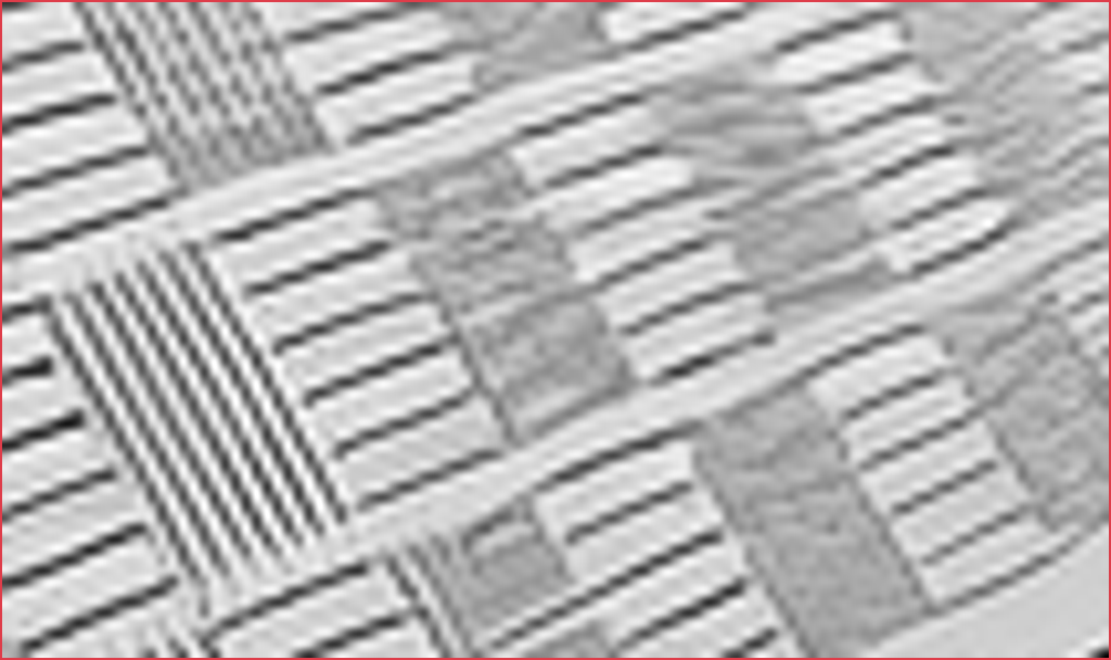
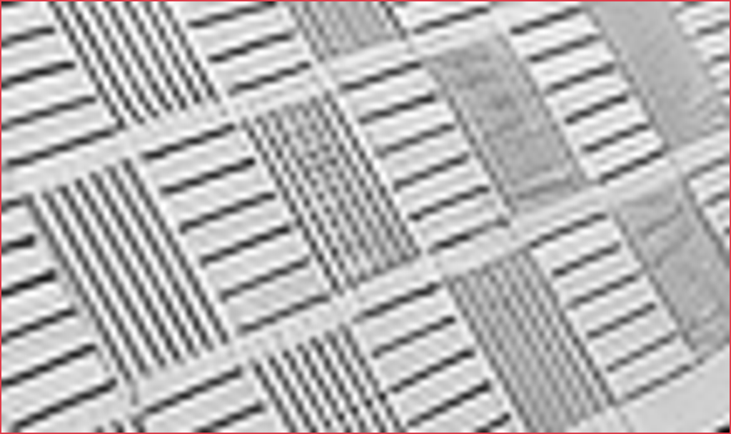
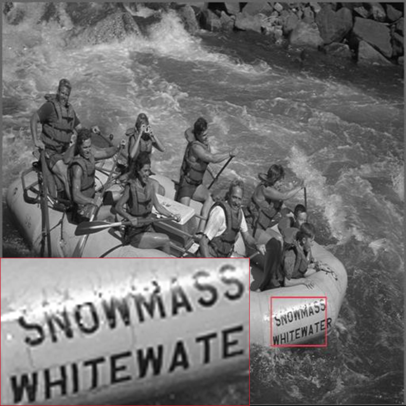
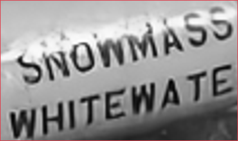
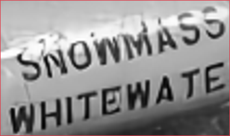
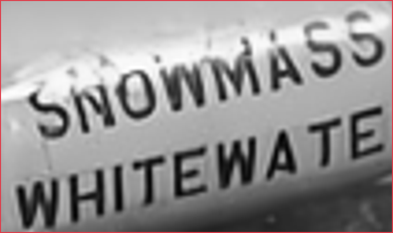
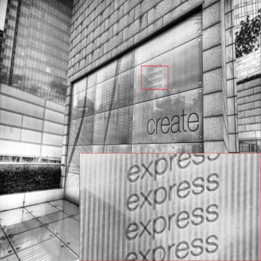
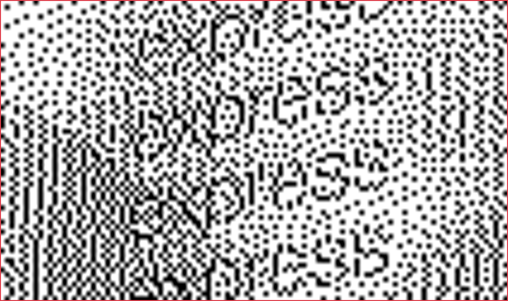
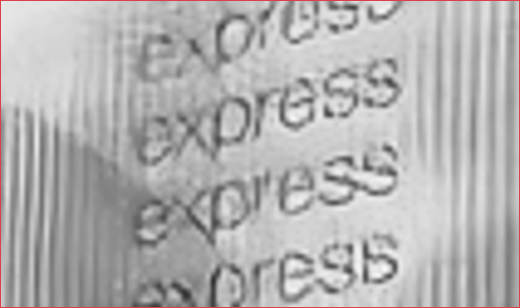
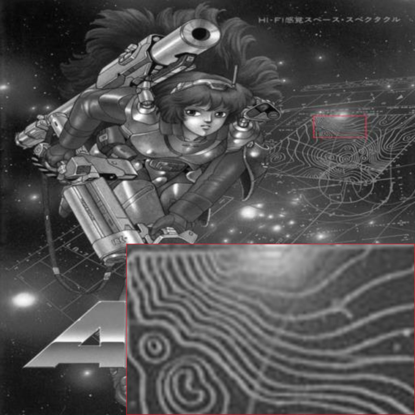
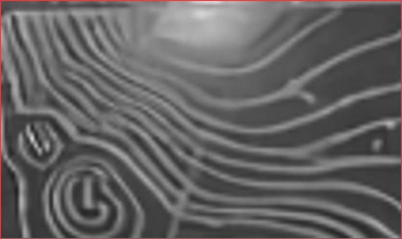
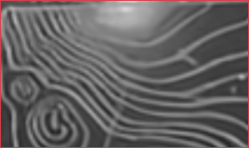
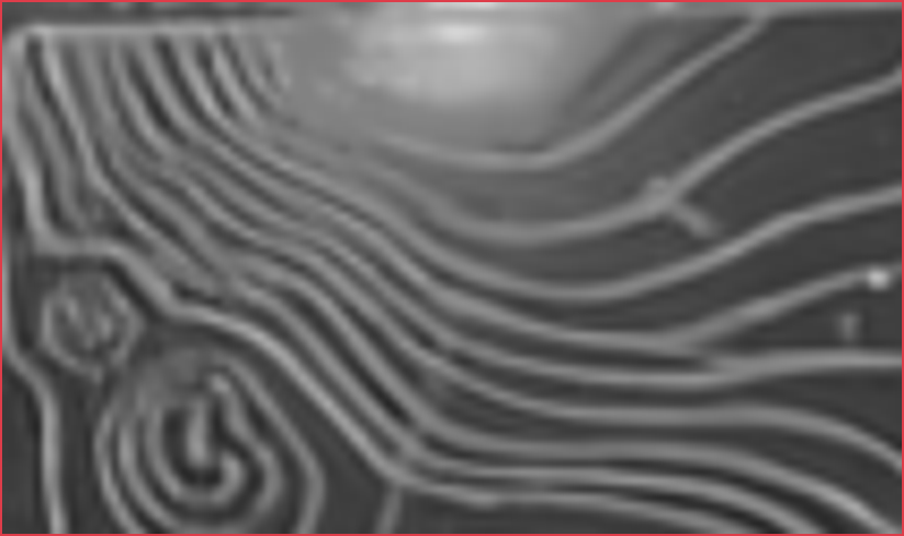
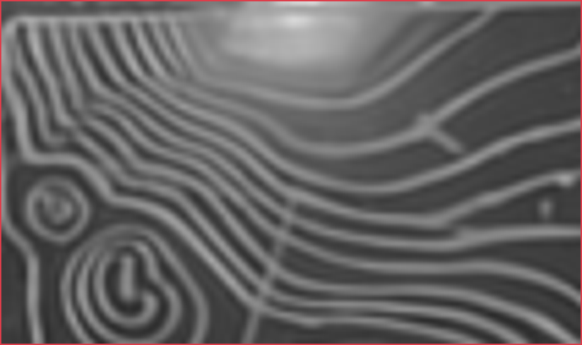
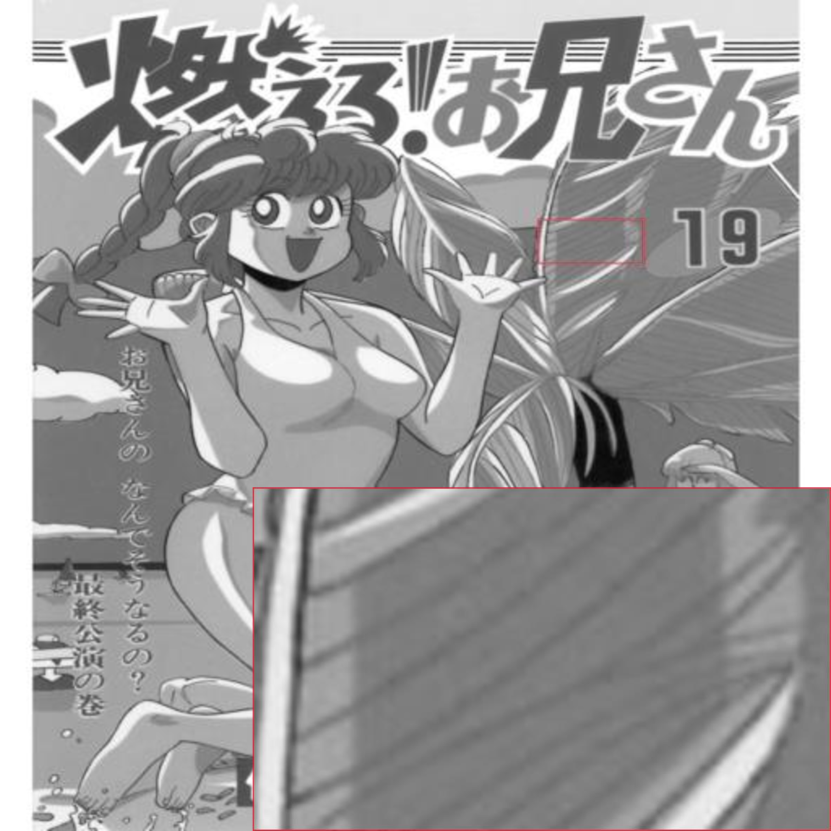
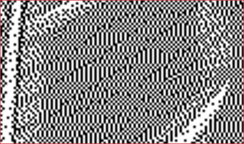
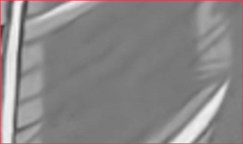
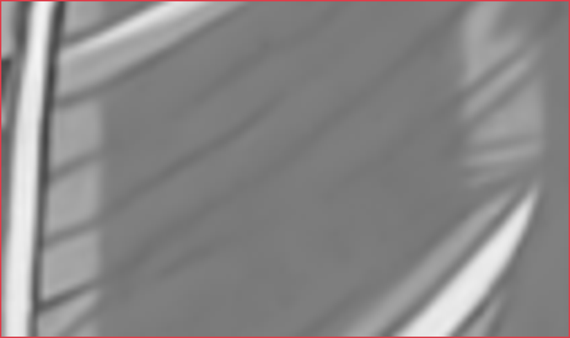
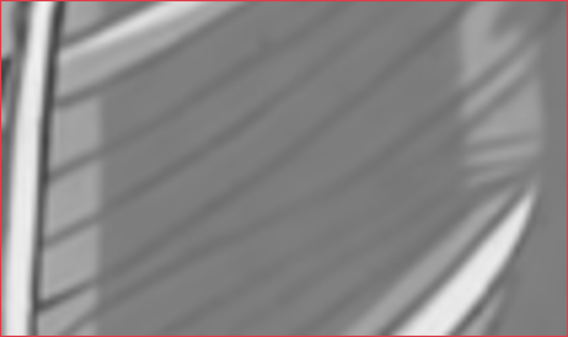
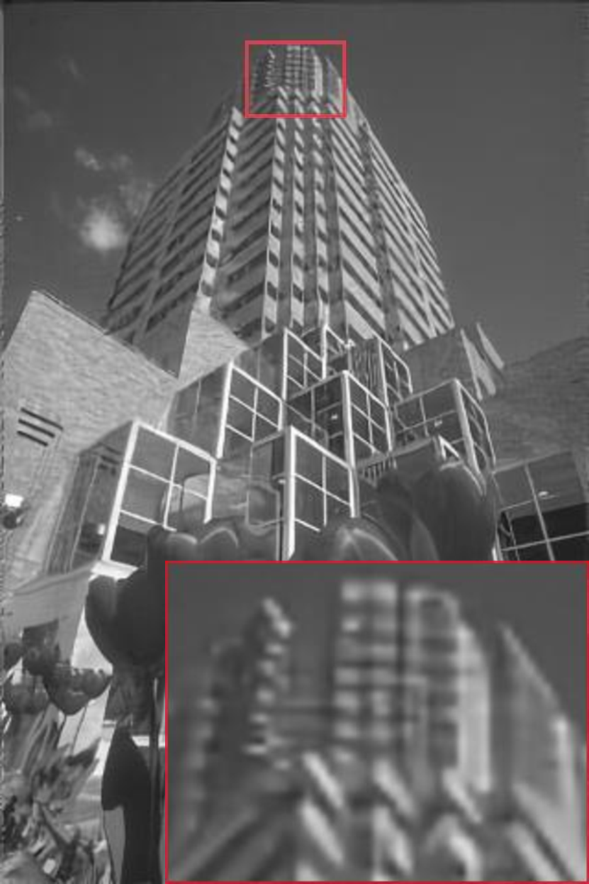
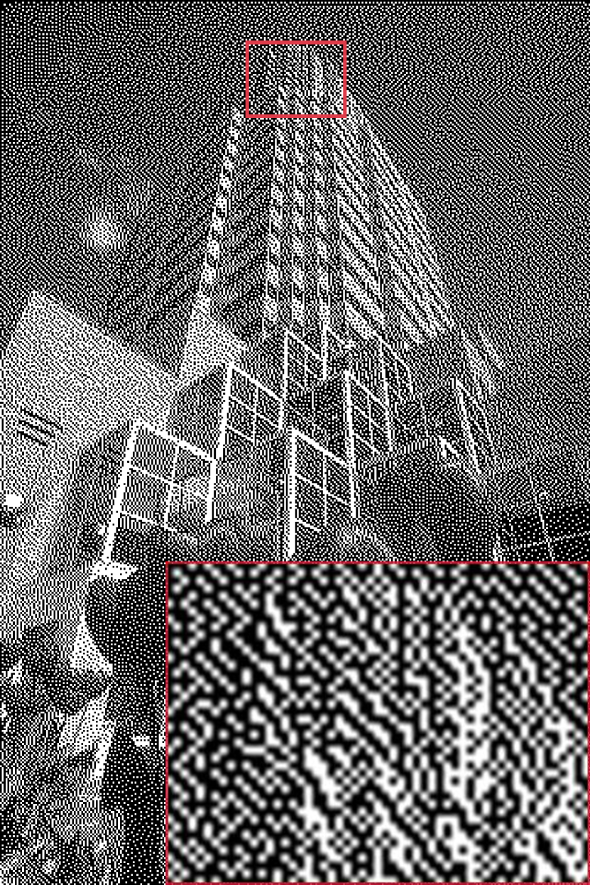
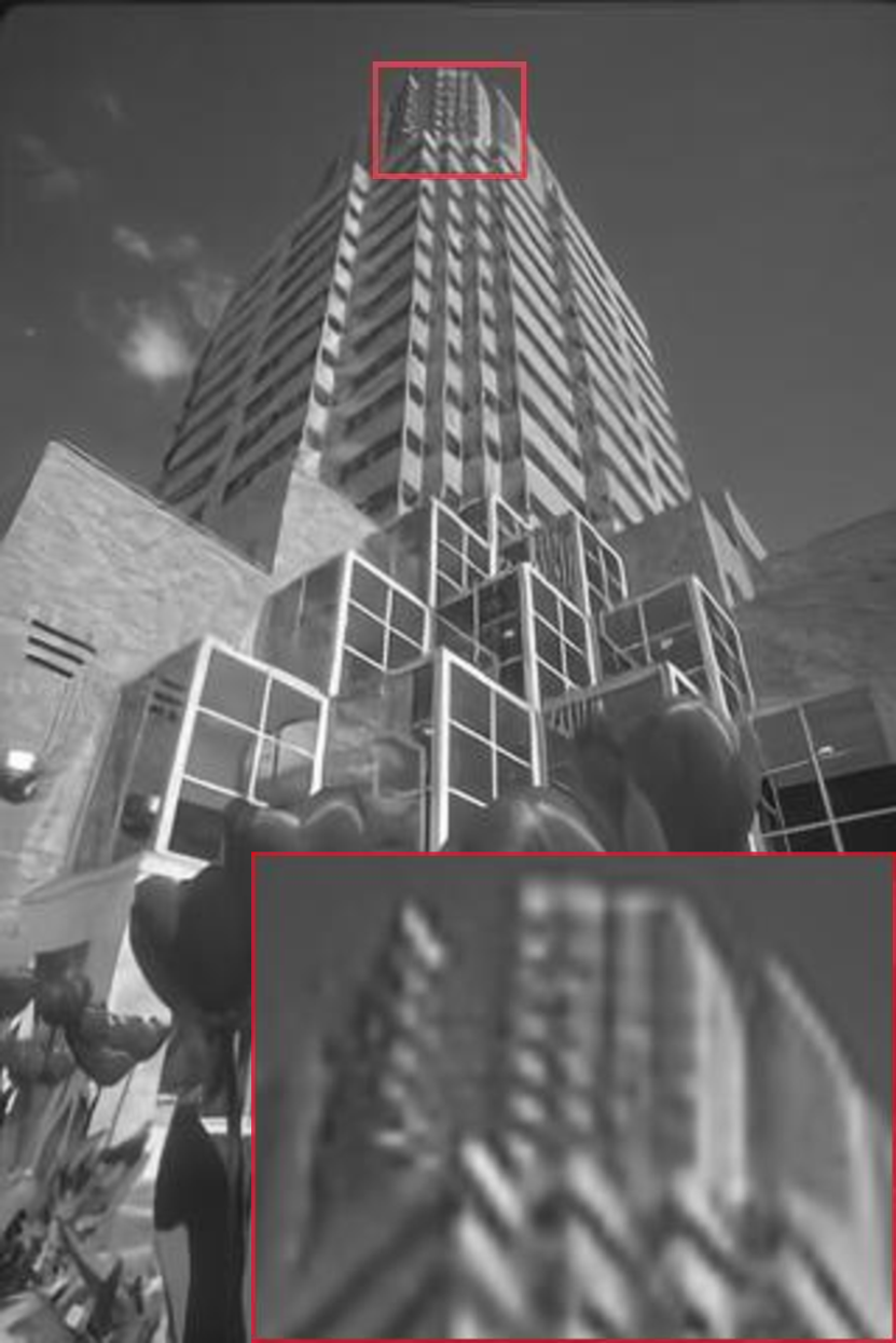
We show the visual comparisons in Fig. 6. Our MSPRL can obtain more obvious texture and structure information than PRL-dt, which effectively restores the image details. In the Lena image, the hat texture can be well restored using MSPRL, which is closer to the original real image. And, in the Barbara image, the cloth texture restoration of the other models shows more bending phenomena. In Fig. 7 (Row 2, 3 and 4), other models cannot restore the dense circle and point shape of the image, showing the line shape in different directions, while MSPRL can avoid this problem and reconstruct the image. Compared with other models, although the netted information loss of halftone image is very serious, MSPRL is still able to recover the main details, as shown in Fig. 8. In addition, the restoration visual effects of MSPRL in the architectures, letters and lines are more smooth and refined, which are shown in Fig. 9, Fig. 10, Fig. 11 and Fig. 12. Lastly, we also compare the restoration performance on the classic images shown in Tab. 8.
| Model | DnCNN | VDSR | EDSR | PRL | GGRL | MIMOUNet | PRL-dt | MSPRL |
|---|---|---|---|---|---|---|---|---|
| Baboon | 24.73 | 24.59 | 24.85 | 24.50 | 24.83 | 24.98 | 25.03 | 25.12 |
| Barbara | 29.35 | 28.08 | 29.95 | 29.44 | 30.19 | 30.58 | 30.79 | 31.59 |
| Boat | 31.77 | 31.54 | 31.95 | 31.21 | 31.92 | 32.00 | 32.14 | 32.25 |
| Couple | 31.55 | 31.36 | 31.79 | 30.91 | 31.77 | 31.87 | 31.95 | 32.07 |
| Goldhill | 31.71 | 31.51 | 31.86 | 31.01 | 31.87 | 31.90 | 32.06 | 32.15 |
| House | 38.90 | 38.55 | 39.38 | 36.21 | 39.39 | 39.42 | 39.75 | 39.95 |
| Lena | 34.51 | 34.32 | 34.78 | 33.34 | 34.77 | 34.84 | 35.00 | 35.09 |
| Man | 31.86 | 31.68 | 31.97 | 30.96 | 31.97 | 32.00 | 32.08 | 32.15 |
| Peppers | 34.32 | 34.09 | 34.42 | 33.11 | 34.39 | 34.43 | 34.49 | 34.55 |
| \botrule |
5 Conclusion
In this paper, we present a multiscale progressively residual learning architecture network (MSPRL) for the inverse halftoning task. The encoder restores content information from different scale images and the decoder collects encoder features to extract deep features. The feature maps of the entire model are progressively learned. Our MSPRL is a simple and efficient model that can learn information of different scale images. In addition, we use suitable training strategies compared with many previous CNN-based inverse halftoning methods. We also explored the performance of the model between different settings and feature blocks. The experimental results demonstrate that our method outperforms the other model methods. Recently, many researchers have added colorization tasks to inverse halftoning; we will follow up research to restore better visual perception of color continuous-tone images in the future.
References
- \bibcommenthead
- Analoui and Allebach (1992) Analoui M, Allebach J (1992) New results on reconstruction of continuous-tone from halftone. In: Acoustics, Speech, and Signal Processing, IEEE International Conference on, IEEE Computer Society, pp 313–316
- Bayer (1973) Bayer BE (1973) An optimum method for two-level rendition of continuous tone pictures. In: IEEE International Conference on Communications, June, 1973
- Bevilacqua et al (2012) Bevilacqua M, Roumy A, Guillemot C, et al (2012) Low-complexity single-image super-resolution based on nonnegative neighbor embedding
- Catté et al (1992) Catté F, Lions PL, Morel JM, et al (1992) Image selective smoothing and edge detection by nonlinear diffusion. SIAM Journal on Numerical analysis 29(1):182–193
- Chen et al (2022) Chen L, Chu X, Zhang X, et al (2022) Simple baselines for image restoration. arXiv preprint arXiv:220404676
- Cho et al (2021) Cho SJ, Ji SW, Hong JP, et al (2021) Rethinking coarse-to-fine approach in single image deblurring. In: Proceedings of the IEEE/CVF international conference on computer vision, pp 4641–4650
- Cochran et al (1967) Cochran WT, Cooley JW, Favin DL, et al (1967) What is the fast fourier transform? Proceedings of the IEEE 55(10):1664–1674
- Cubuk et al (2020) Cubuk ED, Zoph B, Shlens J, et al (2020) Randaugment: Practical automated data augmentation with a reduced search space. In: Proceedings of the IEEE/CVF conference on computer vision and pattern recognition workshops, pp 702–703
- Dong et al (2014) Dong C, Loy CC, He K, et al (2014) Learning a deep convolutional network for image super-resolution. In: European conference on computer vision, Springer, pp 184–199
- Eschbach and Knox (1991) Eschbach R, Knox KT (1991) Error-diffusion algorithm with edge enhancement. JOSA A 8(12):1844–1850
- Everingham et al (2015) Everingham M, Eslami SA, Van Gool L, et al (2015) The pascal visual object classes challenge: A retrospective. International journal of computer vision 111:98–136
- Floyd (1976) Floyd RW (1976) An adaptive algorithm for spatial gray-scale. In: Proc. Soc. Inf. Disp., pp 75–77
- Goyal et al (2017) Goyal P, Dollár P, Girshick R, et al (2017) Accurate, large minibatch sgd: Training imagenet in 1 hour. arXiv preprint arXiv:170602677
- Guo et al (2013) Guo JM, Liu YF, Chang JY, et al (2013) Efficient halftoning based on multiple look-up tables. IEEE transactions on image processing 22(11):4522–4531
- He et al (2016) He K, Zhang X, Ren S, et al (2016) Deep residual learning for image recognition. In: Proceedings of the IEEE conference on computer vision and pattern recognition, pp 770–778
- He et al (2019) He T, Zhang Z, Zhang H, et al (2019) Bag of tricks for image classification with convolutional neural networks. In: Proceedings of the IEEE/CVF conference on computer vision and pattern recognition, pp 558–567
- Hendrycks and Gimpel (2016) Hendrycks D, Gimpel K (2016) Gaussian error linear units (gelus). arXiv preprint arXiv:160608415
- Hou and Qiu (2017) Hou X, Qiu G (2017) Image companding and inverse halftoning using deep convolutional neural networks. arXiv preprint arXiv:170700116
- Huang et al (2015) Huang JB, Singh A, Ahuja N (2015) Single image super-resolution from transformed self-exemplars. In: Proceedings of the IEEE conference on computer vision and pattern recognition, pp 5197–5206
- Huang et al (2008) Huang WB, Su AW, Kuo YH (2008) Neural network based method for image halftoning and inverse halftoning. Expert Systems with Applications 34(4):2491–2501
- Kim et al (2016) Kim J, Lee JK, Lee KM (2016) Accurate image super-resolution using very deep convolutional networks. In: Proceedings of the IEEE conference on computer vision and pattern recognition, pp 1646–1654
- Kingma and Ba (2014) Kingma DP, Ba J (2014) Adam: A method for stochastic optimization. arXiv preprint arXiv:14126980
- Kite et al (2000) Kite TD, Damera-Venkata N, Evans BL, et al (2000) A fast, high-quality inverse halftoning algorithm for error diffused halftones. IEEE Transactions on Image Processing 9(9):1583–1592
- Knuth (1987) Knuth DE (1987) Digital halftones by dot diffusion. ACM Transactions on Graphics (TOG) 6(4):245–273
- Lim et al (2017) Lim B, Son S, Kim H, et al (2017) Enhanced deep residual networks for single image super-resolution. In: Proceedings of the IEEE conference on computer vision and pattern recognition workshops, pp 136–144
- Lin et al (2022) Lin Z, Garg P, Banerjee A, et al (2022) Revisiting rcan: Improved training for image super-resolution. arXiv preprint arXiv:220111279
- Liu et al (2010) Liu YF, Guo JM, Lee JD (2010) Inverse halftoning based on the bayesian theorem. IEEE Transactions on Image Processing 20(4):1077–1084
- Loshchilov and Hutter (2016) Loshchilov I, Hutter F (2016) Sgdr: Stochastic gradient descent with warm restarts. arXiv preprint arXiv:160803983
- Loshchilov and Hutter (2017) Loshchilov I, Hutter F (2017) Decoupled weight decay regularization. arXiv preprint arXiv:171105101
- Maas et al (2013) Maas AL, Hannun AY, Ng AY, et al (2013) Rectifier nonlinearities improve neural network acoustic models. In: Proc. icml, Atlanta, Georgia, USA, p 3
- Martin et al (2001) Martin D, Fowlkes C, Tal D, et al (2001) A database of human segmented natural images and its application to evaluating segmentation algorithms and measuring ecological statistics. In: Proceedings Eighth IEEE International Conference on Computer Vision. ICCV 2001, IEEE, pp 416–423
- Matsui et al (2017) Matsui Y, Ito K, Aramaki Y, et al (2017) Sketch-based manga retrieval using manga109 dataset. Multimedia Tools and Applications 76(20):21,811–21,838
- Mese and Vaidyanathan (2001) Mese M, Vaidyanathan PP (2001) Look-up table (lut) method for inverse halftoning. IEEE Transactions on Image Processing 10(10):1566–1578
- Mulligan and Ahumada Jr (1992) Mulligan JB, Ahumada Jr AJ (1992) Principled halftoning based on human vision models. In: Human vision, visual processing, and digital display III, SPIE, pp 109–121
- Nair and Hinton (2010) Nair V, Hinton GE (2010) Rectified linear units improve restricted boltzmann machines. In: Icml
- Qian et al (2022) Qian G, Li Y, Peng H, et al (2022) Pointnext: Revisiting pointnet++ with improved training and scaling strategies. arXiv preprint arXiv:220604670
- Seldowitz et al (1987) Seldowitz MA, Allebach JP, Sweeney DW (1987) Synthesis of digital holograms by direct binary search. Applied optics 26(14):2788–2798
- Shao et al (2021) Shao L, Zhang E, Li M (2021) An efficient convolutional neural network model combined with attention mechanism for inverse halftoning. Electronics 10(13):1574
- Shi et al (2016) Shi W, Caballero J, Huszár F, et al (2016) Real-time single image and video super-resolution using an efficient sub-pixel convolutional neural network. In: Proceedings of the IEEE conference on computer vision and pattern recognition, pp 1874–1883
- Son and Choo (2014) Son CH, Choo H (2014) Local learned dictionaries optimized to edge orientation for inverse halftoning. IEEE Transactions on Image Processing 23(6):2542–2556
- Unal and Çetin (2001) Unal GB, Çetin AE (2001) Restoration of error-diffused images using projection onto convex sets. IEEE transactions on image processing 10(12):1836–1841
- Wang et al (2018) Wang X, Yu K, Wu S, et al (2018) Esrgan: Enhanced super-resolution generative adversarial networks. In: Proceedings of the European conference on computer vision (ECCV) workshops, pp 0–0
- Wong (1995) Wong PW (1995) Inverse halftoning and kernel estimation for error diffusion. IEEE Transactions on Image Processing 4(4):486–498
- Xia and Wong (2018) Xia M, Wong TT (2018) Deep inverse halftoning via progressively residual learning. In: Asian Conference on Computer Vision, Springer, pp 523–539
- Xia et al (2021) Xia M, Hu W, Liu X, et al (2021) Deep halftoning with reversible binary pattern. In: Proceedings of the IEEE/CVF International Conference on Computer Vision, pp 14,000–14,009
- Xiao et al (2017) Xiao Y, Pan C, Zhu X, et al (2017) Deep neural inverse halftoning. In: 2017 International Conference on Virtual Reality and Visualization (ICVRV), IEEE, pp 213–218
- Yen et al (2021) Yen YT, Cheng CC, Chiu WC (2021) Inverse halftone colorization: Making halftone prints color photos. In: 2021 IEEE International Conference on Image Processing (ICIP), IEEE, pp 1734–1738
- Yuan et al (2019) Yuan J, Pan C, Zheng Y, et al (2019) Gradient-guided residual learning for inverse halftoning and image expanding. IEEE Access 8:50,995–51,007
- Zamir et al (2022) Zamir SW, Arora A, Khan S, et al (2022) Restormer: Efficient transformer for high-resolution image restoration. In: Proceedings of the IEEE/CVF Conference on Computer Vision and Pattern Recognition, pp 5728–5739
- Zeyde et al (2010) Zeyde R, Elad M, Protter M (2010) On single image scale-up using sparse-representations. In: International conference on curves and surfaces, Springer, pp 711–730
- Zhang et al (2017) Zhang K, Zuo W, Chen Y, et al (2017) Beyond a gaussian denoiser: Residual learning of deep cnn for image denoising. IEEE transactions on image processing 26(7):3142–3155
- Zhang et al (2018a) Zhang Y, Li K, Li K, et al (2018a) Image super-resolution using very deep residual channel attention networks. In: Proceedings of the European conference on computer vision (ECCV), pp 286–301
- Zhang et al (2018b) Zhang Y, Zhang E, Chen W, et al (2018b) Sparsity-based inverse halftoning via semi-coupled multi-dictionary learning and structural clustering. Engineering Applications of Artificial Intelligence 72:43–53
- Zhao et al (2016) Zhao H, Gallo O, Frosio I, et al (2016) Loss functions for image restoration with neural networks. IEEE Transactions on computational imaging 3(1):47–57
- Zhou et al (2017) Zhou B, Lapedriza A, Khosla A, et al (2017) Places: A 10 million image database for scene recognition. IEEE Transactions on Pattern Analysis and Machine Intelligence