Retrieving maximum information of symmetric states from their corrupted copies

Using quantum measurements to extract information from quantum states is an indispensable ingredient of quantum information processing, underpinning numerous applications across quantum science and technologies. One primary example is to extract the expectation value $\overline{X}:=\mathrm{tr}(\rho X)$ of an observable $X$ in a state $\rho$ from the quantum measurements performed on $\rho$. A long-standing pursuit in this line of research is to devise efficient methods to reduce sample complexity in quantum measurements, which has led to the proposals of compressed sensing [1, 2], adaptive tomography [3, 4], self-guided tomography [5, 6], and classical shadows [7, 8, 9].

The recent work [10] explored leveraging symmetric structures of states to reduce the sample complexity in measuring expectation values of observables. The state $\rho$ is said to be symmetric under a group $G$ if it satisfies

where $U_{g}$ denotes a unitary representation of $G$. This equation defines the symmetric structures of $\rho$, which are pervasive in quantum physics and frequently encountered in diverse contexts. A salient example showcasing the emergence of symmetric structures arises in condensed-matter physics, where the states of interest commonly exhibit translational symmetries [11]. Another well-known example is in multipartite experiments [12, 13, 14, 15, 16, 17, 18], where the states under consideration often remain invariant under permutations [19, 20, 21]. Notable instances of permutation-invariant states include the Werner states [22], the Dicke states [23], and the Greenberger-Horne-Zeilinger (GHZ) states [24], which are useful resources in quantum information processing tasks [25, 26, 27].

The main finding of Ref. [10] is that, when the state $\rho$ in question exhibits some symmetric structures, the optimal measurement for obtaining $\overline{X}$ is the projective measurement of another observable $Y$ rather than $X$ itself. Here,

where $\mathcal{P}$ is the so-called $G$-twirling operation, defined as $\mathcal{P}\left(X\right)=\sum_{g}{U_{g}XU_{g}^{\dagger}}/\left|G\right|$ for a finite group $G$, with $\left|G\right|$ the cardinality of $G$. When $G$ is a compact Lie group, $\mathcal{P}\left(X\right)=\int_{G}{d\mu\left(g\right)U_{g}XU_{g}^{\dagger}}$, where $\mu(g)$ is the normalized Haar measure [28, 29]. Two key properties of $Y$ are that

but

where $(\Delta X)^{2}:=\tr(\rho X^{2})-(\tr\rho X)^{2}$ is the quantum uncertainty of $X$ and $(\Delta Y)^{2}$ is defined in a similar way. Physically, the equality (3) means that the projective measurement of $Y$ can be an alternative to the projective measurement of $X$ for obtaining $\overline{X}$. The inequality (4) implies that the former generally consumes fewer samples than the latter for reaching the same measurement precision.

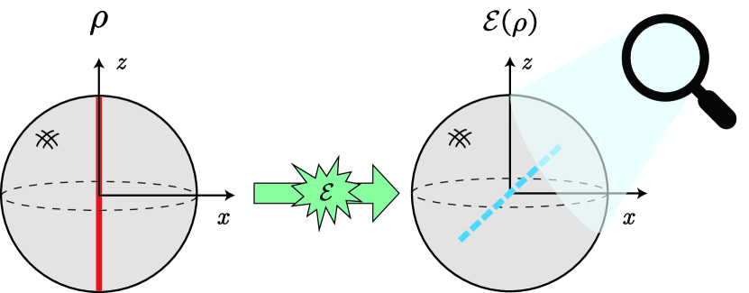
The purpose of the present study is to complement the recent work [10] by taking into account noise, which can be, without loss of generality, modeled by a completely positive and trace-preserving map $\mathcal{E}$. As a persistent topic in quantum information science [30, 31], the state $\rho$ may be corrupted by noise before the execution of quantum measurements [32, 33]. This leads to the fact that the actual state available in the presence of noise is the corrupted state $\mathcal{E}(\rho)$ rather than $\rho$ itself (see Fig. 1 for a schematic illustration). A natural question then arises: How can we optimally measure the expectation value $\overline{X}=\tr(\rho X)$ of $X$ in $\rho$ when the actual state at hand is $\mathcal{E}(\rho)$? This question is highly nontrivial as the symmetric structures described by Eq. (1) are distorted in $\mathcal{E}(\rho)$.

In this study we answer this question. The information content we use is the quantum Fisher information (QFI) [Braunstein1994PRL, Zhang2020PRR], the inverse of which characterizes the optimal sample complexity in quantum measurements according to the celebrated quantum Cramér-Rao bound [10]. Moreover, it makes sense to say that the QFI is the maximal information extractable via a quantum measurement, as the classical Fisher information naturally characterizes the information extracted from a measurement and the QFI, by definition, is the maximal classical Fisher information over all measurements. To identify the optimal measurement capable of extracting the QFI, we resort to the geometric formulation of parameter estimation theory [TAD20], which is well suited for dealing with the estimation of a parameter that can be expressed as a function of $\rho$, such as the expectation value of an observable, the fidelity to a given pure state, and the von Neumann entropy. Resorting to this theory, we show that the optimal measurement can be found by solving a semidefinite program (SDP) whenever the noise model $\mathcal{E}$ is invertible.¹¹1As a linear map on the space of Hermitian operators, $\mathcal{E}$ can be described by a matrix if we choose a basis for this space. By saying that $\mathcal{E}$ is invertible, we mean that the matrix associated with $\mathcal{E}$ is invertible. Intuitively speaking, a non-invertible $\mathcal{E}$ arises in the situation that the information about the initial state $\rho$ is lost and cannot be retrieved [ZJZ24]. As the aim of this paper is to retrieve information from corrupted copies of $\rho$, we focus on the setting that $\mathcal{E}$ is invertible. However, it turns out that this measurement may depend on $\rho$, due to which a refined knowledge of $\rho$ may be required in order to implement it in practice. We clarify that such an unpleasant dependence issue is a common feature in quantum metrology rather than being exclusive to the present study.

To release the requirement on the knowledge of $\rho$, we further specialize our discussions to a large class of noise models that are covariant under the symmetry group $G$. The studies on covariant quantum operations have been extensive and garnered significant interest because of their relevance in various physical contexts. For example, the absence of a quantum reference frame such as a phase or Cartesian reference frame imposes constraints on a party’s ability to prepare states and perform quantum operations. This has sparked a line of development known as quantum reference frames [BRS07], where covariant quantum operations are those that can be executed without access to a reference frame. Another example is the presence of superselection rules [WWW52, BW03], which restricts the permissible quantum operations on a quantum system to be covariant ones. More generally, the presence of symmetries in a system generally imposes restrictions on the manipulation of the system, which results in nontrivial limitations on the implementation of quantum operations [MS14, PCB16, ZYHT17]. This has led to the proposal of the resource theory of asymmetry [GS08, CG19], where covariant quantum operations are the free operations that do not consume or increase the asymmetry resource of states. We show that the optimal measurement can be explicitly determined for covariant models, thereby eliminating the dependence issue mentioned above.

Finally, we apply our results to an experimentally relevant scenario, demonstrating how to optimally take advantage of the distorted symmetric structures in $\mathcal{E}(\rho)$ to reduce the sample complexity in information retrieval.

This paper is organized as follows. In Sec. II, we set the stage of our analysis. In Sec. III, we show how to find the optimal measurement whenever the noise model $\mathcal{E}$ is invertible. In Sec. IV, we specialize our discussion to the noise models that are covariant under the group $G$. We apply our results to an experimentally relevant scenario in Sec. V and conclude this paper in Sec. VI.

We are interested in the QFI about $\overline{X}$ given $\mathcal{E}(\rho)$ [10], denoted as $\mathcal{J}[\overline{X};\mathcal{E}(\rho)]$, which represents the maximal information about $\overline{X}$ that we can extract from $\mathcal{E}(\rho)$ via a quantum measurement [Hel76, Hol11]. To specify the form of $\mathcal{J}[\overline{X};\mathcal{E}(\rho)]$, we recall that the $\rho$ satisfying Eq. (1) can be parametrized using the representation theory of groups [10]. That is, $\rho$ can be expressed as $\rho(\bm{\theta})$ for some parameters $\bm{\theta}=(\theta_{1},\cdots,\theta_{q})$, where $q$ denotes an integer. For example, a qubit state respecting the symmetry group $G=\{\mathbb{1},\sigma_{z}\}$ can be expressed as $\rho=\textrm{diag}(\theta,1-\theta)$, where $\sigma_{\alpha}$, $\alpha=x,y,z$, denote the Pauli matrices. The explicit form of $\rho(\bm{\theta})$ in general can be found in Supplemental Material of Ref. [10] and is presented in Appendix A of the present study, too. Apparently, $\mathcal{E}(\rho)$ also depends on $\bm{\theta}$ and $\overline{X}=\tr(\rho X)$ can be regarded as a function of $\bm{\theta}$. We can express $\mathcal{J}[\overline{X};\mathcal{E}(\rho)]$ as [10]

where $\partial\overline{X}:=(\frac{\partial\overline{X}}{\partial\theta_{1}},\cdots,\frac{\partial\overline{X}}{\partial\theta_{q}})^{T}$ is a $q$-dimensional vector, and $H$ denotes the QFI matrix whose $ij$ element is given by

Here $S_{i}$ is known as symmetric logarithmic derivative (SLD) [Hel76, Hol11], defined as the Hermitian operator that satisfies

Below, we find a convenient formula for calculating $\mathcal{J}[\overline{X};\mathcal{E}(\rho)]$. We do this by following the theory in Ref. [TAD20].

Throughout this study, we only consider Hermitian operators unless otherwise specified. We define a weighted inner product²²2Strictly speaking, this definition represents a pre-inner product as the positive-definiteness requirement may not be met when $\mathcal{E}(\rho)$ is singular. between two operators $h_{1}$ and $h_{2}$ as

where the subscript $\mathcal{E}(\rho)$ is used to indicate the dependence of this definition on $\mathcal{E}(\rho)$. Equation (8) induces a norm

which inherits the dependence on $\mathcal{E}(\rho)$ from the inner product.

We introduce a linear space of zero-mean operators as

It is easy to see that all the SLDs defined by Eq. (LABEL:SLD) belong to $\mathcal{Z}_{\mathcal{E}(\rho)}$. Therefore, the linear span of these SLDs

is a subspace of $\mathcal{Z}_{\mathcal{E}(\rho)}$. $\mathcal{T}_{\mathcal{E}(\rho)}$ is known as the tangent space in the estimation theory in Ref. [TAD20]. We also introduce

which is the orthogonal complement of $\mathcal{T}_{\mathcal{E}(\rho)}$ in the space $\mathcal{Z}_{\mathcal{E}(\rho)}$.

A useful notion in the theory [TAD20] is the so-called influence operator, defined as an operator $\delta$ in $\mathcal{Z}_{\mathcal{E}(\rho)}$ that satisfies

for $i=1,...,q$. Such an operator may not be unique. We choose

with $\mathbb{1}$ denoting the identity matrix. Here we have assumed that $\mathcal{E}$ is invertible. $\mathcal{E}^{*}$ denotes the dual map³³3Let $\mathcal{E}(\rho)=\sum_{i}K_{i}\rho K_{i}^{\dagger}$ be the Kraus representation of $\mathcal{E}$, where $K_{i}$’s are Kraus operators. Then the dual map $\mathcal{E}^{*}$ can be expressed as $\mathcal{E}^{*}(h)=\sum_{i}K_{i}^{\dagger}hK_{i}$. of $\mathcal{E}$ [Zhang2016PRA]; that is, $\mathcal{E}$ and $\mathcal{E}^{*}$ satisfy the relation $\tr[h_{1}\mathcal{E}(h_{2})]=\tr[\mathcal{E}^{*}(h_{1})h_{2}]$. It is a general property that $\mathcal{E}^{*}$ is invertible if and only if $\mathcal{E}$ is invertible. $\mathcal{E}^{*-1}$ denotes the inverse of $\mathcal{E}^{*}$. We prove in Appendix B that $\delta$ defined in Eq. (14) is indeed a legitimate influence operator.

According to Theorem 1 in Ref. [TAD20], the QFI $\mathcal{J}[\overline{X};\mathcal{E}(\rho)]$ can be evaluated using the influence operator:

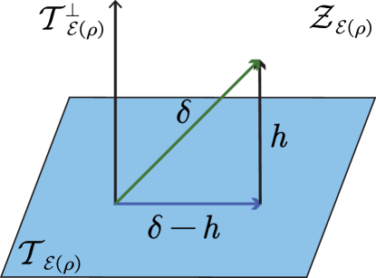
which is the convenient formula we seek. We schematically show the concepts introduced above in Fig. 2.

To find the optimal measurement, we now convert formula (15) into an SDP. We do this in the following three steps.

Let us now consider the setting that $\mathcal{E}$ is covariant under the group $G$, which is of relevance in a plethora of physical contexts as mentioned in the introduction [BRS07, WWW52, BW03, MS14, PCB16, ZYHT17, GS08, CG19]. Formally, $\mathcal{E}$ is said to be covariant with respect to $G$ if

for all $g\in G$ and Hermitian operators $h$ [MS14, PCB16, ZYHT17]. In what follows, we show how to explicitly determine the optimal measurement of $Y_{h_{0}}$ for these covariant noise models.

We first show that $\mathcal{P}$ and $\mathcal{E}^{*-1}$ are exchangeable, that is,

for any $h$. To see why Eq. (42) holds, we can sum both sides of Eq. 41 over the group elements $g$ in $G$, and obtain

for all $h$. That is, the two maps $\mathcal{P}$ and $\mathcal{E}$ are exchangeable. This implies that $\mathcal{P}$ and $\mathcal{E}^{*-1}$ are exchangeable, which can be verified by resorting to the matrix representation of $\mathcal{E}$, $\mathcal{P}$, and $\mathcal{E}^{*-1}$. Indeed, let $\left\{H_{i}\right\}$ denote a Hermitian basis. In this basis, the linear map $\mathcal{E}$ can be represented by the matrix $A_{\mathcal{E}}$ whose $ij$th element is given by

Then, by the cyclic property of the trace, we have that

which implies that $A_{\mathcal{E}}^{T}=A_{\mathcal{E}^{*}}$. Additionally, $A_{\mathcal{P}}$ is symmetric since

Combining these facts, we have that the commutativity $\left[A_{\mathcal{P}},A_{\mathcal{E}}\right]=0$, which follows from Eq. (43), implies that $\left[A_{\mathcal{P}}^{T},A_{\mathcal{E}}^{T}\right]=\left[A_{\mathcal{P}},A_{\mathcal{E}^{*}}\right]=0$. Furthermore, using the identity $A_{\mathcal{E}^{*-1}}=A_{\mathcal{E}^{*}}^{-1}$, we conclude that $\left[A_{\mathcal{P}},A_{\mathcal{E}^{*-1}}\right]=0$ as well, that is, $\mathcal{P}$ and $\mathcal{E}^{*-1}$ are exchangeable. Noting that

we deduce from Eq. (42) that $\mathcal{Q}$ and $\mathcal{E}^{*-1}$ are exchangeable, too.

We then show that $\mathcal{P}$ is idempotent and Hermitian with respect to the inner product in Eq. (8), that is, $\mathcal{P}$ satisfies

and

for any operators $h_{1}$ and $h_{2}$. Equation (48) follows directly from the fact that $\mathcal{P}(h_{1})$ is invariant under the action of $U_{g}$, i.e., $U_{g}\mathcal{P}(h_{1})U_{g}^{\dagger}=\mathcal{P}(h_{1})$. To verify Eq. (49), we note that

which leads to

as $\mathcal{E}$ is covariant under $G$ and $\rho$ is symmetric. Analogously, we have

Then Eq. (49) follows from summing the two sides of Eqs. 51 and 52. A direct consequence of Eqs. (48) and (49) is

which can be verified by noting that $\mathcal{P}(\mathcal{Q}(h))=\mathcal{P}(h)-\mathcal{P}(\mathcal{P}(h))=0$.

Let us now determine $Y_{h_{0}}$. To do this, we use the equality

to rewrite Eq. (38) as

Note that $Y_{h}$ can be expressed as

Exchanging $\mathcal{E}^{*-1}$ with $\mathcal{P}$ and $\mathcal{Q}$ in Eq. (56), we have that

Inserting Eq. (57) into Eq. (55) and using Eq. (53), we obtain

Apparently, $h=X$ attains the minimum and $Y_{h_{0}}=\mathcal{P}(\mathcal{E}^{*-1}(X))=\mathcal{E}^{*-1}(\mathcal{P}(X))$. We therefore arrive at the following theorem:

We see that the observable $\mathcal{E}^{*-1}\left(\mathcal{P}\left(X\right)\right)$ is independent of $\rho$, which means that the aforementioned dependence issue is eliminated in Theorem 2. We clarify that Theorem 2 holds for any covariant quantum operation $\mathcal{E}$ and any choice of $X$. It is worth noting that a special covariant quantum operation is $\mathcal{E}=\textrm{id}$, which corresponds to the noiseless situation considered in Ref. [10]. We easily deduce from Theorem 2 that $Y_{h_{0}}=\mathcal{P}(X)$ in this situation, which is one of the key findings of Ref. [10]. Besides, to better digest the result in Theorem 2, we provide an intuitive understanding of this result in Appendix E.

To demonstrate the usefulness of our results, we now consider the setting that $\rho$ is an $n$-qubit state whose symmetric structures are described by $G=\{P_{\pi},\pi\in S_{n}\}$. Here $\pi$ labels the permutations in the symmetric group $S_{n}$ and $P_{\pi}$ is the unitary representation of $\pi$, defined by

with $|\psi_{i}\rangle\in\mathbb{C}^{2}$. Such states naturally arise in multipartite experiments [12, 13, 14, 15, 16, 17, 18]. A well-known example is the Dicke states

where $\textrm{wt}(x)$ is the number of ones in $x$, e.g., $\textrm{wt}(x)=1$ when $x=010$.

Motivated by the fact that dephasing is one of the dominant types of noise encountered in experiments [PRG19, ZBH19, ZZW22], we set $\mathcal{E}$ to be the dephasing noise acting independently on the $n$ qubits. Specifically, the dephasing noise acting on a single qubit is described by the channel

where $p$ quantifies the noise strength. Here we assume that $0\leq p<1$, since the dephasing channel is not invertible at $p=1$. The noise model $\mathcal{E}$ can be described as

A direct calculation shows that the map $\mathcal{E}^{*-1}$ reads

Notably, $\mathcal{E}$ is covariant under $G$, which implies that Theorem 2 can be applied in the setting under consideration.

To demonstrate the superiority of the projective measurement of the observable $\mathcal{E}^{*-1}\left(\mathcal{P}\left(X\right)\right)$, which is the optimal measurement according to Theorem 2, we would like to compare it with the projective measurement of the observable $\mathcal{E}^{*-1}(X)$. The latter measurement, referred to as the customary measurement hereafter, has been studied in Ref. [WSU10]. It is interesting to note that

that is, the expectation value of $\mathcal{E}^{*-1}(X)$ in $\mathcal{E}(\rho)$ is equal to $\overline{X}$. Hence, both the optimal measurement identified here and the customary measurement can be employed to measure $\overline{X}$. The interesting difference between them is that

that is, the quantum uncertainty of $\mathcal{E}^{*-1}\left(\mathcal{P}\left(X\right)\right)$ in $\mathcal{E}(\rho)$ is generally smaller than the quantum uncertainty of $\mathcal{E}^{*-1}(X)$.

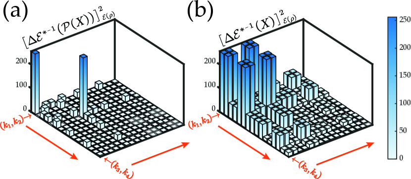
To explicitly see the difference, we consider the task of measuring the expectation values of Pauli observables

where $\sigma_{k_{i}}\in\left\{\sigma_{x},\sigma_{y},\sigma_{z},\sigma_{I}\right\}$ with $\sigma_{I}=\mathbb{1}$. Figure 3 shows the values of the two quantum uncertainties when $\rho$ is the four-qubit Dicke state $\ket{D_{4}^{(2)}}$. The labels $(k_{1},k_{2})$ and $(k_{3},k_{4})$, which appear aside the two horizontal axes in Fig. 3, correspond to the observable $X_{k1,k2,k3,k4}$ in Eq. (66). As can be seen from Fig. 3, $[\Delta\mathcal{E}^{*-1}(\mathcal{P}(X))]_{\mathcal{E}(\rho)}^{2}$ is significantly smaller than $[\Delta\mathcal{E}^{*-1}(X)]_{\mathcal{E}(\rho)}^{2}$ for most of the $256$ Pauli observables. Specifically, we find that the ratio

for all the Pauli observables except for the trivial ones, $\sigma_{\alpha}^{\otimes 4}$, $\alpha=I,x,y,z$, which are invariant under $\mathcal{P}$, i.e., $\mathcal{P}(\sigma_{\alpha}^{\otimes 4})=\sigma_{\alpha}^{\otimes 4}$. We see from Eq. (67) that the optimal measurement, when used to measure $\overline{X}$ for these observables, requires only $37\%$ of the copies of $\mathcal{E}(\rho)$ compared with the customary measurement to achieve the same precision.

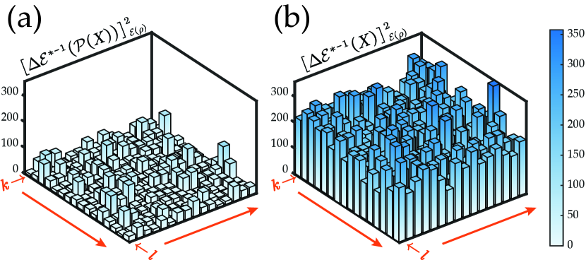
To demonstrate that the superiority of our measurement is not exclusive to the 256 Pauli observables considered above, we further randomly generate 256 new observables, $X_{k,l}$, with $k,l=1,2,\cdots,16$. Here, each observable is produced by randomly generating a complex matrix $C$ and then setting $X$ to be $\left(C+C^{\dagger}\right)/2$. Figure 4 shows the two quantum uncertainties for the randomly generated observables, where $\rho$ is set to be the Dicke state $\ket{D_{4}^{(2)}}$, too. As can be seen from this figure, the quantum uncertainty associated with the optimal measurement is significantly smaller than the customary one for all the observables. Specifically, the ratio reads

with an average value of $0.14$. We have randomly generated multiple sets of $256$ observables and obtained similar results, although the specific numbers appearing in Eq. (68) may be different when different sets are in question.

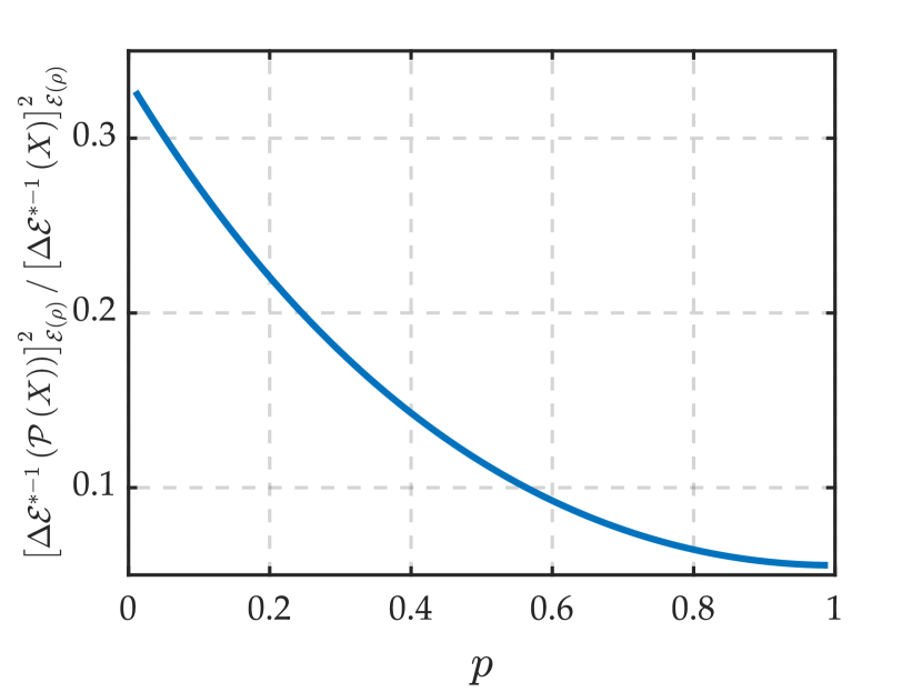
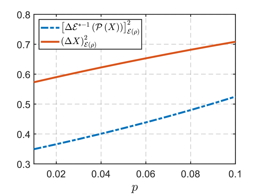
Besides, we examine the ratio between the two quantum uncertainties as a function of the noise strength $p$. As can be seen from Fig. 5, the ratio becomes increasingly small in the course of varying $p$ from $0.01$ to $0.99$. This means that the superiority of our measurement becomes increasingly significant as the noise strength increases. Moreover, we also numerically examine the performance of the projective measurement of $X$ in the low-noise regime, which may provide an approximately unbiased estimate of $\overline{X}$. The numerical result is presented in Fig. 6, showing that $\left[\Delta\mathcal{E}^{*-1}\left(\mathcal{P}\left(X\right)\right)\right]_{\mathcal{E}\left(\rho\right)}^{2}$ is also smaller than $\left(\Delta X\right)_{\mathcal{E}\left(\rho\right)}^{2}$ when $p$ varies from $0.01$ to $0.1$.

We have identified the measurement capable of retrieving the maximum information about the expectation value $\overline{X}$ of an observable $X$ in $\rho$ from the corrupted state $\mathcal{E}(\rho)$. Our general result, presented in Theorem 1, shows that this measurement is the projective measurement of $Y_{h_{0}}$, which can be found by solving the SDP in Eq. (40). As the QFI is employed to quantify the information content, Theorem 1 is of fundamental importance and characterizes the optimal sample complexity in estimating $\overline{X}$ according to the quantum Cramér-Rao bound [10].

To eliminate the dependence of $Y_{h_{0}}$ on $\rho$, we have shown that $Y_{h_{0}}$ can be explicitly determined for covariant noise models, as stated in Theorem 2. This result reduces to one of the key findings in Ref. [10], which can find immediate applications due to the relevance of covariant noise models in various contexts. We have demonstrated the usefulness of our result by applying Theorem 2 to the scenario that involves permutation symmetries.

We clarify that, while the local parameter estimation theory provides powerful tools like the QFI, it also produces the inherent drawback that $Y_{h_{0}}$ may depend on $\rho$ [PAR09]. To overcome this drawback, one may resort to the global parameter estimation theory, such as the Bayesian and minimax approaches [Per71, GL95, Hay11, MFD14, RD19, DGG20, GDWB20, RD20, SK20, GD22, BLSM24, Rub24], which can single out a globally optimal measurement that is independent of $\rho$. It is worth noting that a recent study [ZQZ24] has established a link between the local and global parameter estimation theories, which could be a valuable reference for future efforts to fully resolve the dependence issue.

References

- Gross et al. [2010] D. Gross, Y.-K. Liu, S. T. Flammia, S. Becker, and J. Eisert, Quantum State Tomography via Compressed Sensing, Phys. Rev. Lett. 105, 150401 (2010).
- Liu et al. [2012] W.-T. Liu, T. Zhang, J.-Y. Liu, P.-X. Chen, and J.-M. Yuan, Experimental Quantum State Tomography via Compressed Sampling, Phys. Rev. Lett. 108, 170403 (2012).
- Mahler et al. [2013] D. H. Mahler, L. A. Rozema, A. Darabi, C. Ferrie, R. Blume-Kohout, and A. M. Steinberg, Adaptive Quantum State Tomography Improves Accuracy Quadratically, Phys. Rev. Lett. 111, 183601 (2013).
- Qi et al. [2017] B. Qi, Z. Hou, Y. Wang, D. Dong, H.-S. Zhong, L. Li, G.-Y. Xiang, H. M. Wiseman, C.-F. Li, and G.-C. Guo, Adaptive quantum state tomography via linear regression estimation: Theory and two-qubit experiment, npj Quantum Inf. 3, 19 (2017).
- Ferrie [2014] C. Ferrie, Self-Guided Quantum Tomography, Phys. Rev. Lett. 113, 190404 (2014).
- Rambach et al. [2021] M. Rambach, M. Qaryan, M. Kewming, C. Ferrie, A. G. White, and J. Romero, Robust and Efficient High-Dimensional Quantum State Tomography, Phys. Rev. Lett. 126, 100402 (2021).
- Aaronson [2018] S. Aaronson, Shadow tomography of quantum states, in Proceedings of the 50th Annual ACM SIGACT Symposium on Theory of Computing (ACM, New York, 2018) pp. 325–338.
- Huang et al. [2020] H.-Y. Huang, R. Kueng, and J. Preskill, Predicting many properties of a quantum system from very few measurements, Nat. Phys. 16, 1050 (2020).
- Huang et al. [2021] H.-Y. Huang, R. Kueng, and J. Preskill, Efficient Estimation of Pauli Observables by Derandomization, Phys. Rev. Lett. 127, 030503 (2021).
- Zhang and Tong [2024] D.-J. Zhang and D. M. Tong, Inferring Physical Properties of Symmetric States from the Fewest Copies, Phys. Rev. Lett. 133, 040202 (2024).
- Zhou and Zhang [2023] L. Zhou and D.-J. Zhang, Non-Hermitian Floquet Topological Matter—A Review, Entropy 25, 1401 (2023).
- Kiesel et al. [2007] N. Kiesel, C. Schmid, G. Tóth, E. Solano, and H. Weinfurter, Experimental Observation of Four-Photon Entangled Dicke State with High Fidelity, Phys. Rev. Lett. 98, 063604 (2007).
- Wieczorek et al. [2008] W. Wieczorek, C. Schmid, N. Kiesel, R. Pohlner, O. Gühne, and H. Weinfurter, Experimental Observation of an Entire Family of Four-Photon Entangled States, Phys. Rev. Lett. 101, 010503 (2008).
- Wieczorek et al. [2009] W. Wieczorek, R. Krischek, N. Kiesel, P. Michelberger, G. Tóth, and H. Weinfurter, Experimental Entanglement of a Six-Photon Symmetric Dicke State, Phys. Rev. Lett. 103, 020504 (2009).
- Prevedel et al. [2009] R. Prevedel, G. Cronenberg, M. S. Tame, M. Paternostro, P. Walther, M. S. Kim, and A. Zeilinger, Experimental Realization of Dicke States of up to Six Qubits for Multiparty Quantum Networking, Phys. Rev. Lett. 103, 020503 (2009).
- Krischek et al. [2010] R. Krischek, W. Wieczorek, A. Ozawa, N. Kiesel, P. Michelberger, T. Udem, and H. Weinfurter, Ultraviolet enhancement cavity for ultrafast nonlinear optics and high-rate multiphoton entanglement experiments, Nature Photon. 4, 170 (2010).
- Erhard et al. [2018] M. Erhard, M. Malik, M. Krenn, and A. Zeilinger, Experimental Greenberger–Horne–Zeilinger entanglement beyond qubits, Nature Photon. 12, 759 (2018).
- Liu et al. [2021] Z.-H. Liu, J. Zhou, H.-X. Meng, M. Yang, Q. Li, Y. Meng, H.-Y. Su, J.-L. Chen, K. Sun, J.-S. Xu, C.-F. Li, and G.-C. Guo, Experimental test of the Greenberger–Horne–Zeilinger-type paradoxes in and beyond graph states, npj Quantum Inf. 7, 66 (2021).
- Tóth et al. [2010] G. Tóth, W. Wieczorek, D. Gross, R. Krischek, C. Schwemmer, and H. Weinfurter, Permutationally Invariant Quantum Tomography, Phys. Rev. Lett. 105, 250403 (2010).
- Moroder et al. [2012] T. Moroder, P. Hyllus, G. Tóth, C. Schwemmer, A. Niggebaum, S. Gaile, O. Gühne, and H. Weinfurter, Permutationally invariant state reconstruction, New J. Phys. 14, 105001 (2012).
- Gao et al. [2014] T. Gao, F. Yan, and S. van Enk, Permutationally Invariant Part of a Density Matrix and Nonseparability of -Qubit States, Phys. Rev. Lett. 112, 180501 (2014).
- Werner [1989] R. F. Werner, Quantum states with Einstein-Podolsky-Rosen correlations admitting a hidden-variable model, Phys. Rev. A 40, 4277 (1989).
- Dicke [1954] R. H. Dicke, Coherence in Spontaneous Radiation Processes, Phys. Rev. 93, 99 (1954).
- Greenberger et al. [1989] D. M. Greenberger, M. A. Horne, and A. Zeilinger, Bell’s Theorem, Quantum Theory, and Conceptions of the Universe, edited by M. Kafatos (Kluwer Academics, Dordrecht, The Netherlands, 1989).
- Horodecki et al. [2009] R. Horodecki, P. Horodecki, M. Horodecki, and K. Horodecki, Quantum entanglement, Rev. Mod. Phys. 81, 865 (2009).
- Gühne and Tóth [2009] O. Gühne and G. Tóth, Entanglement detection, Phys. Rep. 474, 1 (2009).
- Hu et al. [2018] M.-L. Hu, X. Hu, J. Wang, Y. Peng, Y.-R. Zhang, and H. Fan, Quantum coherence and geometric quantum discord, Phys. Rep. 762, 1 (2018).
- Halmos [1950] P. R. Halmos, Measure Theory (Springer-Verlag, New York, 1950).
- Mele [2024] A. A. Mele, Introduction to Haar Measure Tools in Quantum Information: A Beginner’s Tutorial, Quantum 8, 1340 (2024).
- Preskill [2018] J. Preskill, Quantum Computing in the NISQ era and beyond, Quantum 2, 79 (2018).
- Jiao et al. [2023] L. Jiao, W. Wu, S. Bai, and J. An, Quantum Metrology in the Noisy Intermediate-Scale Quantum Era, Adv. Quantum Technol. 2023, 2300218 (2023).
- Zhang and Tong [2022] D.-J. Zhang and D. M. Tong, Approaching Heisenberg-scalable thermometry with built-in robustness against noise, npj Quantum Inf. 8, 81 (2022).
- Ullah et al. [2023] A. Ullah, M. T. Naseem, and O. E. Müstecaplioğlu, Low-temperature quantum thermometry boosted by coherence generation,