Revealing the nature of hidden charm pentaquarks with machine learning
Abstract
We study the nature of the hidden charm pentaquarks,
i.e. the , and , with a neural network approach in
pionless effective field theory. In this framework, the normal fitting approach
cannot distinguish the quantum numbers of the and .
In contrast to that, the neural network-based approach can discriminate them, which still cannot be seen as a proof of the spin of the states since pion exchange is not considered in the approach.
In addition, we also illustrate the role of each experimental data bin of the invariant mass distribution
on the underlying physics in both neural network and fitting methods.
Their similarities and differences demonstrate that neural network methods
can use data information more effectively and directly.
This study provides more insights about how the neural network-based approach
predicts the nature of exotic states from the mass spectrum.
Keywords: Exotic hadrons, Machine learning, QCD mass spectrum
I Introduction
In the last two decades, we have witnessed the emergence of tens of candidates for the so-called exotic hadrons which are beyond the conventional meson and baryon configurations, such as the hidden charm pentaquarks [1, 2, 3], the fully charmed tetraquark [4, 5, 6], or the doubly charmed tetraquark [7, 8]. The first hidden charm pentaquarks were reported by the LHCb Collaboration in 2015 in Ref. [1] by observing the invariant mass via the process . Four years later, the , and were reported with an order of magnitude larger luminosity in Ref. [3]. Since then, many interpretations have been proposed for these states, e.g. compact multi-quark, hadronic molecule, hybrid, and triangle singularity [9, 10, 11, 12, 13, 14, 15, 16, 17, 16, 18, 19, 20]. Traditionally, judging whether a model works or not is to compare it with the experimental data. However, such a top-down approach makes the conclusion model-dependent. Physicists are thus trying to find bottom-up approaches [21] to obtain a definitive conclusion. One direction is to use machine learning to explore hadron properties, which benefits from the evolution of computing capabilities during the last decades. For instance, genetic algorithms [22, 23, 24] and neural networks [25, 26, 27, 28] can be utilized to explore the nature of hadrons or the properties of nuclei. Machine learning has been widely used in nuclear physics [29, 30, 31, 32, 33, 34, 35], high energy nuclear physics [36, 37, 38], experimental data analysis [39, 40], and theoretical physics [41, 42], even to discover the physical principles underneath the experimental data [21, 43, 44]. However, its application in hadron physics is in the early stage. A preliminary attempt was made in Refs. [45, 46, 21, 47] for the hadronic molecular picture [12], which is one of the natural explanations of near-threshold peaks. Refs. [48, 47] demonstrate that deep learning can be applied to classify poles and regress the model parameters in the one-channel coupling case.
Here, extending and improving the works [45, 46], we consider the multi-channel coupling case. We take the hidden charm pentaquarks, i.e. , and [3] as examples, to achieve the following goals:
-
(1)
In the hadronic molecular picture [49, 50, 51], both the and the are related to the threshold. Their spin-parity () could be either (solution A) or (solution B) [49, 50, 51], from the viewpoint of pionless effective field theory (EFT). In solution A, the lower mass hidden charm pentaquark has lower spin, and vice versa in solution B. Although the fitting cannot distinguish the two solutions, we try to find out which solution is preferred in machine learning.
-
(2)
In the traditional fitting approach, the physics is embedded in the model parameters. One has to extract the model parameters from the experimental data and further extract the physical quantities of interest. We use a neural network (NN) based approach to extract the pertinent physical quantities directly and illustrate the role of each experimental data point (here the bins in the mass distributions) in the physics.
We have used one particular NN for the above goals and demonstrated that the NN-based approach consistently favors solution A over B compared to the fitting approach, and clearly gives the properties of the poles in the multi-channel case.
II Model Description
The and states are close to the and thresholds, respectively, making them prime candidates for hadronic molecules. In the heavy quark limit, these hidden charm pentaquarks are related to the scattering between the and the heavy quark spin doublets. Note that the heavy quark symmetry breaking effect is about in the charm sector, with and the masses of the and mesons. Since both the and are related to the channel, their mass difference comes from the spin-spin interaction between the baryon and the meson for a given total spin, which should vanish in the exact heavy quark limit. Thus in the heavy quark limit the and should coincide with each other. Their hyperfine splitting stems from the heavy quark symmetry breaking effect. Consequently, we consider the heavy quark symmetry breaking effect from the mass difference in the same doublet. By constructing the interactions between the two doublets, i.e. the and the doublets, in the EFT respecting the heavy quark spin symmetry (HQSS), Refs. [51, 50] extracted the pole positions of the seven hidden charm pentaquarks by fitting the invariant mass distribution for the process 111Note that there is additional dynamic channel in Ref. [51] in comparison with Ref. [50]. However, the parameters of the channel are out-of-control due to the absence of the experimental data in the channel and the properties of the poles are driven by the channel. As the result, we only consider the elastic channel and the inelastic , channels in our framework. . Following the same procedure, we consider the and , channels as elastic and inelastic channels, respectively. The potential quantum numbers of hidden charm pentaquarks are and which correspond to the scattering of the , and , respectively. In the heavy quark limit, their interaction only depends on the light degrees of freedom [52]. To extract their interactions, one can expand the two-hadron basis in terms of the heavy-light basis , with and the heavy and light degrees of freedom, respectively,
| (1) |
| (2) |
| (3) |
Here, the subscripts , and give the total spin of the two-hadron system. In the HQSS, as the interaction only depends on the light degrees of freedom [52], the scattering amplitude is described by the two parameters [51]
| (4) | |||||
| (5) |
with the subscripts corresponding to the spin of the light degrees of freedom. The coupling for the -wave and -wave inelastic channels, i.e. the and channels, are described by two parameters
| (6) | |||||
| (7) |
respectively. The weak bare production amplitude can also be parameterized in terms of the basis
| (8) |
with the th state in the basis for spin . With this definition, the bare decay amplitudes read
| (9) |
| (10) |
| (11) |
with the upper index for the total spin of the two-hadron system. Putting pieces together, the inelastic amplitude of the for the decay process can be expressed as [51, 50]
| (12) |
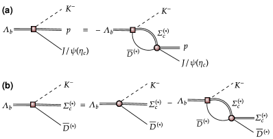
The corresponding diagrams are shown in Fig. 1a. Here, is the th inelastic channel amplitude with the quantum number . is the transition vertex between the th elastic and the th inelastic channel, and described by the coupling constants for the -wave and for the -wave.
| (13) |
is the two-body propagator of the th elastic channel [51, 50], with and the reduced mass and threshold of the th channel. The physical production amplitude of the th elastic channel for total spin is obtained from the Lippmann-Schwinger (LSE)
| (14) |
with , constructed by seven parameters defined as in Eq. (8), the production amplitude for the th elastic channel. The corresponding diagrams are shown in Fig. 1b.
Note that the above integral equations can be reduced to algebric equations in the framework of a pionless EFT. For a general introduction to this type of EFT, see [53]. is the effective potential
| (15) |
which contains both the scattering between the elastic channels described by two parameters , and that between the elastic and inelastic channels described by the two parameters , . In total, eleven parameters are combined in a vector
| (16) | |||||
To describe the invariant mass distribution, a composite model is constructed via a probability distribution function (PDF) as:
| (17) |
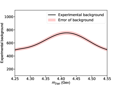
with the amplitude (14) for total spin and is the phase space of the corresponding process. A Gaussian function which represents the experimental detector resolution is convoluted with the physical invariant mass distribution. Here, we take the energy resolution as a constant of MeV [3] without considering its energy dependence. Further, is the sixth-order Chebyshev polynomial which represents the background distribution, with its fraction, . The background fraction in the data is determined to be (96.00.8)% as discussed in the Supplementary materials. The coefficients () for the background component are obtained by fitting the Chebyshev polynomials to data [54], as listed in the Supplementary materials. Note that the area enclosed by the signal (background) distribution, i.e. the remnant of the first term after removing the factor (the second term after removing the factor ) in Eq. (17) is normalized to one.
III States and Labels
The hidden charm pentaquarks are described as generated from the scattering of the and doublets. As the thresholds of the inelastic channels and are far away from those of elastic channels, their effects on the classification of the poles relevant to the physical observables are marginal. Thus, we consider the classification of poles by considering the elastic channels. In this case, the and states are given by a three-channel case with Riemann surfaces denoted as , see [20] for a pictorial. Here, the “+” and “” signs in the th position mean the physical and unphysical sheet of the th channel, respectively. The physical observables, i.e. the invariant mass distribution in our case, are real, reflecting the amplitude in the real axis. Those are related to the poles on the complex plane. We consider the poles most relevant to the physical observables, i.e. the poles on the physical sheet and those close-by ones. As we aim at extracting the most important information of those poles, it is sufficient to work with leading order contact interactions. In this case, the poles accounting for the near threshold structures can be classified as in Fig. 2. For the classification 222For the classification of poles, strictly, bound states do not decay to any final particles, which means them stable. However, in the standard model, there are only 11 stable particles, i.e. photon, the three generations of neutrino and antineutrino, electron, positron, proton, and antiproton. Other particles can decay into final states with lower masses. In our case, bound state, virtual state, and resonance are defined based on the most coupled elastic channels. of the states, we start from the one-channel case, i.e. state related to the channel. The “bound state”, “resonance”, and “virtual state” are defined as a pole on the physical sheet below threshold, a pole on the unphysical sheet above the threshold, and a pole on the unphysical sheet below the threshold, respectively (Fig. 2a). Those poles are labeled as , , in order. For the three-channel case (Fig. 2b), i.e. and channels, the poles are defined according to the most strongly coupled channel. The case with three poles on the , and sheets slightly below the first, second, and third thresholds, respectively, is defined as a “bound state” which is labeled as . The case with three poles on the , and sheets slightly above the first, second, and third thresholds, respectively, is defined as a “resonance” which is labeled as . The case with three poles on the , and sheets slightly below the first, second, and third thresholds, respectively, is defined as a “virtual state” which is labeled as . Note that these three states are defined according to their most strongly coupled channel, which the word “slightly” means. For instance, on the sheet , both the “resonance” (blue circle point) and “bound state” (green crossed point) locate between the first and the second thresholds.
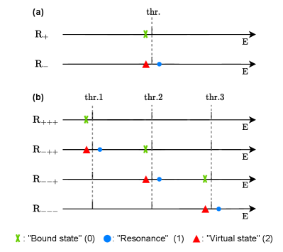
However, the former one strongly couples to the first channel and is located close to the first threshold, defined as a resonance of the first channel. The latter one strongly couples to the second channel and is located close to the second threshold, defined as a bound state of the second channel. The situation for the other states is similar.
We use a four-digit label , with and , to denote the situation of the poles. The last three labels are for the nature of the poles in the and channels in order. The first label “”, which we put in front, is used for the mass order. That is due to the indeterminacy of the quantum numbers of the and . As they are close to the threshold, the -wave interaction can give both and states. In the limit of HQSS, there are two solutions, i.e. Solution A and Solution B defined in Refs. [49, 50, 51], as discussed before. In Solution A, the higher spin state has larger mass, i.e. and . In Solution B, the situation is reversed, i.e. and . To distinguish these two scenarios, another label and for Solution A and Solution B, respectively, is required. In total, we have a four-digit label “” to denote the situation of the poles. Taking the “1012” case for example, it means that the poles for and channels are “bound state”, “resonance” and “virtual state”, respectively. The first label means Solution A, i.e. . Note that we can also have cases with the poles different from the three situations discussed above, e.g. the poles are far away from the thresholds. However, their probabilities are almost zero and are thus neglected.
IV Monte Carlo simulation
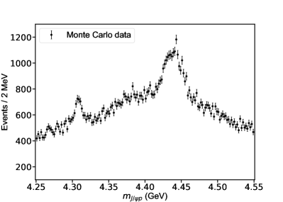
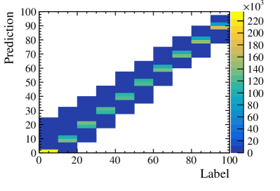
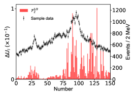
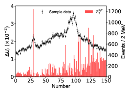
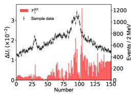
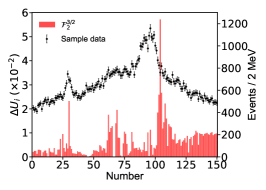
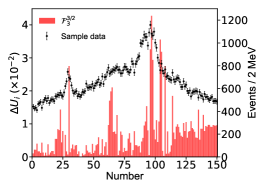
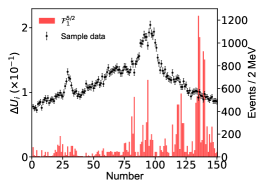
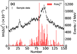
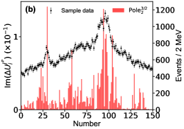
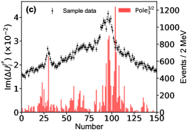
Based on the PDF given in Eq. (17), 240184 samples corresponding to physical states, i.e. with poles not too far away from the real axis in the considered energy range, are selected among 1.85 million samples uniformly generated in the space of , distributed in the mass window from 4.25 to 4.55 . These samples are represented as a set: where the index refers to a given sample. A histogram with 150 bins (see Fig. 3) denotes the invariant mass spectrum of the states (background included) and the label indicates the state label defined in Sec. III.
The values of are uniformly sampled in the following ranges,
| (18) | |||||
The ranges are empirically taken to produce a mass spectrum similar to the experimental data. Note that and as well as and are strongly correlated, so the second of these coefficients is related by a factor in the range to the corresponding first one. Note that these strong correlations were found in Refs. [50, 51], and are also found if one uses a much larger set of samples to train the NNs. The Monte Carlo (MC) production is performed with the open source software ROOT [54] and GSL [55], as categorized in Tab. 1. Considering different background fractions, the set of MC samples produced at the background fraction 90% is denoted as , so are the other sets.
| Mass relation label | State label | Number of samples |
| 0 | 000 | 46,951 |
| 1 | 000 | 4283 |
| 1 | 001 | 1260 |
| 1 | 002 | 4360 |
| 0 | 100 | 3740 |
| 0 | 110 | 4320 |
| 0 | 111 | 7520 |
| 1 | 111 | 360 |
| 0 | 200 | 9590 |
| 1 | 200 | 280 |
| 1 | 210 | 3980 |
| 1 | 211 | 2690 |
| 1 | 220 | 50,240 |
| 1 | 221 | 50,512 |
| 1 | 222 | 50,098 |
V Training and Verification
The NN is implemented with an infrastructure of ResNet [56] as discussed in the Supplementary materials, and solved with the Adam [57] optimizer parametrized by the cross-entropy loss function. In order to balance the impact of unequal sample sizes, the cross-entropy loss function is weighted by the reciprocal of the number of samples. To avoid the network falling into a local minimum solution during the training process, the weights of the neurons are randomly initialized with a normal distribution centered at 0 and with a width of 0.01, and the biases of the neurons are set to zero. A reasonable solution can be obtained after training 500 epochs, using an initial learning rate value of 0.001.
Here the learning rate of the next interval is reduced to half of the previous one, controlled by the stepLR method. The interval is set to 100 epochs in our case. Note that 70% of MC simulation samples are used for training and the rest 30% for a benchmark. To avoid overfitting in the training, dropout layers are introduced in the network during the training. The dropout probability is chosen to 0.3 to optimise performance. In case of overfitting, the obtained NN works well on training datasets while probably does not on testing datasets. Thus the loss function calculated with training datasets should obviously differ from the one calculated with testing datasets. However, Fig. 9 in the Supplementary materials indicates that there is no obvious difference. The training details are summarized in the Supplementary materials. In short, the NNs successfully retrieve the state label with an accuracy (standard deviation) of 75.91(1.18)%, 73.14(1.05)%, 65.25(1.80)% and 54.35(2.32)% for MC simulation samples , , and . The prediction accuracy decreases as the background increases, as expected.
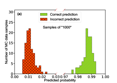
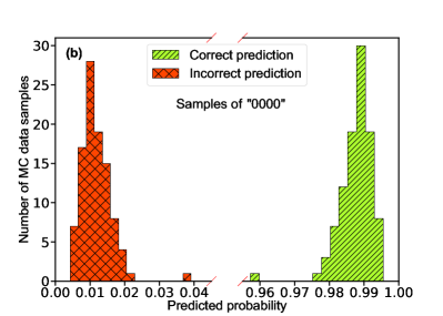
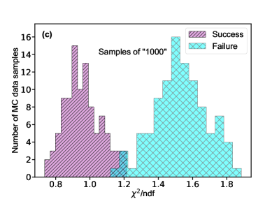
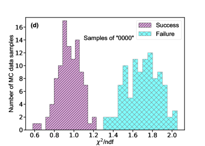
Turning to the mass relation, we verified 100 samples corresponding to the label “1xxx”, and another 100 samples corresponding to the label “0xxx”. Fig. 4a/b shows the predicted probability distribution for the label “1xxx/0xxx” samples, in which all labels are successfully retrieved. In other words, the NN can accurately predict the mass relationship. For comparison, we also perform an analysis with the /ndf-fitting method. Fig. 4c/d shows the normalized /ndf distributions corresponding to the label “1xxx/0xxx”. A 3% misidentification is observed for the label “1xxx” samples.
VI Application to Data
We now use the well-trained NNs to analyse the experimental data. The results are listed in Tab. 2. To reduce the systematic uncertainties arising from the NNs, we trained five and ten NN models, which have an identical structure under different initialization, for each group of samples with different background fractions. The probabilities of the sum of all the other labels are smaller than 1%. The labels with the top three probabilities are “1000”, “1001” and “1002”, with the sum of them larger than . The standard deviation decreases with the increasing number of NN models, as expected. It means that our NNs can well determine the first three labels and favors Solution A, i.e. and , as the first label is .
| Models | Label | |||||
| 0000 | 1000 | 1001 | 1002 | 100X | Others | |
| Prediction(%) of NN trained with samples. | ||||||
| NN 1 | 0.69 | 89.13 | 1.42 | 8.75 | 99.30 | 0.01 |
| NN 2 | 0.03 | 5.83 | 38.47 | 55.30 | 99.60 | 0.37 |
| NN 3 | 0.03 | 5.39 | 15.79 | 78.41 | 99.59 | 0.11 |
| NN 4 | 0.01 | 1.9 | 27.01 | 70.95 | 99.86 | 0.13 |
| NN 5 | 2.40 | 94.45 | 0.15 | 2.99 | 97.59 | 0.01 |
| 5 NNs average | 0.63(1.03) | 39.34 | 16.57 | 43.28 | 99.19(0.91) | 0.13(0.15) |
| 10 NNs average | 0.36(0.74) | 21.16 | 20.69 | 57.62 | 99.47(0.68) | 0.12(0.13) |
| Prediction(%) of NN trained with samples. | ||||||
| NN 1 | 0.00 | 0.15 | 5.37 | 94.47 | 99.99 | 0.00 |
| NN 2 | 0.00 | 0.07 | 4.11 | 95.81 | 99.99 | 0.00 |
| NN 3 | 0.00 | 0.78 | 13.57 | 85.61 | 99.96 | 0.03 |
| NN 4 | 0.00 | 0.81 | 19.02 | 80.16 | 99.99 | 0.00 |
| NN 5 | 0.14 | 15.13 | 16.91 | 67.80 | 99.84 | 0.00 |
| 5 NNs average | 0.03(0.06) | 3.39 | 11.80 | 84.77 | 99.95(0.06) | 0.01(0.01) |
| 10 NNs average | 0.01(0.04) | 1.78 | 9.50 | 88.70 | 99.97(0.04) | 0.00(0.01) |
| Prediction(%) of NN trained with samples. | ||||||
| NN 1 | 0.00 | 1.20 | 2.26 | 96.53 | 99.99 | 0.00 |
| NN 2 | 0.02 | 2.23 | 11.51 | 86.24 | 99.98 | 0.00 |
| NN 3 | 0.00 | 0.26 | 10.26 | 89.47 | 99.99 | 0.00 |
| NN 4 | 0.15 | 24.05 | 48.79 | 26.89 | 99.73 | 0.13 |
| NN 5 | 0.02 | 4.12 | 72.61 | 23.23 | 99.96 | 0.02 |
| 5 NNs average | 0.04(0.06) | 6.37 | 29.09 | 64.47 | 99.93(0.11) | 0.03(0.06) |
| 10 NNs average | 0.02(0.05) | 4.25 | 26.00 | 69.70 | 99.95(0.08) | 0.02(0.04) |
| Prediction(%) of NN trained with samples. | ||||||
| NN 1 | 0.00 | 1.29 | 19.79 | 78.92 | 100.00 | 0.00 |
| NN 2 | 0.00 | 3.38 | 25.64 | 70.97 | 99.99 | 0.01 |
| NN 3 | 0.00 | 6.57 | 32.20 | 61.23 | 100.00 | 0.00 |
| NN 4 | 0.60 | 55.77 | 21.65 | 21.96 | 99.38 | 0.00 |
| NN 5 | 0.00 | 0.27 | 3.52 | 96.20 | 99.99 | 0.00 |
| 5 NNs average | 0.12(0.27) | 13.46 | 20.56 | 65.86 | 99.87(0.28) | 0.00(0.01) |
| 10 NNs average | 0.11(0.21) | 13.13 | 24.97 | 61.79 | 99.89(0.22) | 0.00(0.01) |
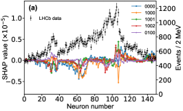
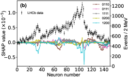
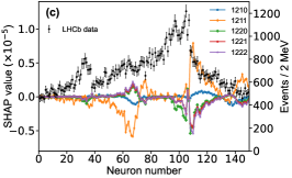
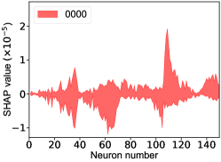
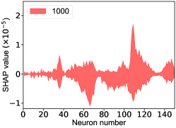
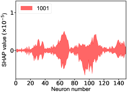
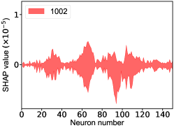
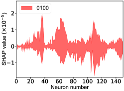
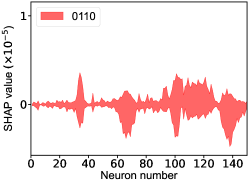
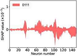
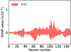
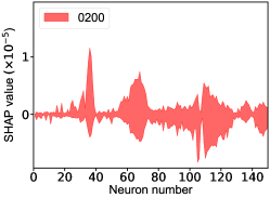
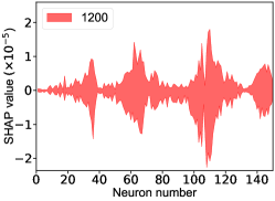
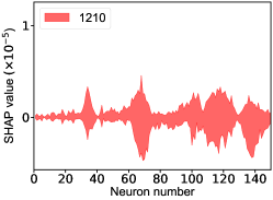
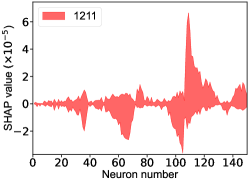
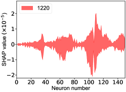
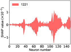
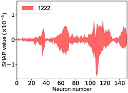
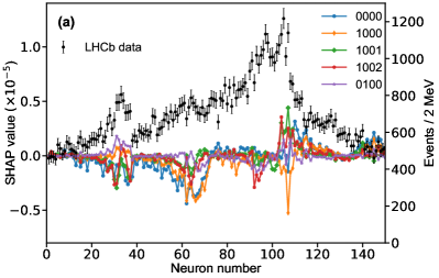
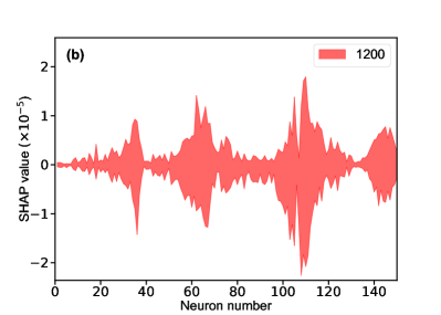
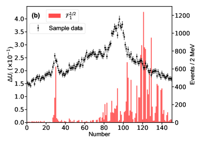
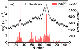
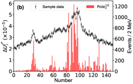
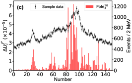
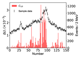
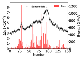
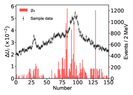
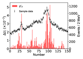
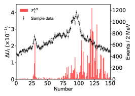
That shows one of the advantages of machine learning comparing to the normal fitting approach. However, this conclusion is only based on the pionless EFT. One cannot obtain a solid conclusion about the hadronic molecules without the one-pion-exchange (OPE) potential. Thus it makes little sense to compare our results with that of Refs. [51, 50]. However, the hidden charm pentaquarks in pionless EFT are sufficient to illustrate the difference between machine learning and the normal fitting approach, as well as the potential merit of machine learning. The second label and the third label mean that the poles for the and channels behave as “bound states”, which is different from the virtual state conclusion for the in Ref. [21] also using machine learning. The pole situation for the is undetermined, i.e. all of the three labels , , appearing for the fourth label, as the structure around the is not significant. To resolve this issue, precise data in this energy region would be needed. In the normal fitting approach, the =1/2, 3/2 and 5/2 channels are described by the same set of parameters in the heavy quark limit. As the result, once the set of parameters is determined, all the poles of the three channels are determined as well. However, in our NN approach, we extract the types of poles without extracting the intermediate parameters directly from the experimental data. This makes the poles of the =1/2, 3/2 well determined, but the =5/2 channel undetermined. Of importance is to understand how the NN learns information from the input mass spectrum . The SHapley Additive exPlanation (SHAP) value is widely used as a feature importance metric for well-established models in machine learning. One of the prevailing methods for estimating NN model features is the DeepLIFT algorithm based on DeepExplainer. A positive (negative) SHAP value indicates that a given data point is pushing the NN classification in favor of (against) a given class. A large absolute SHAP value implies a large impact of a given mass bin on the classification. This method requires a certain amount of dataset as a reference for evaluating network features. We choose 3000 {} samples in the dataset as a reference to test the SHAP values of both 1000 {} samples and the experimental data on our network. The upper panel of Fig. 18 shows the SHAP values of experimental data corresponding to 5 labels, i.e. “0000”, “1001”, “0100”, “1000” and “1002”. The lower panel of Fig. 18 shows the SHAP values of MC samples corresponding to the “1200” label, with others presented in the Supplementary materials. Both panels of Fig. 18 indicate that data points around the peaks in the mass spectrum have a greater impact.
A comparison is performed by checking the traditional /ndf-fitting approach, which minimizes the
| (19) |
between the theoretical prediction and experimental data by summing over all bins of , where represents the model parameters to be determined and is the bin index. We check how the th bin of impacts on the parameters and the pole positions.
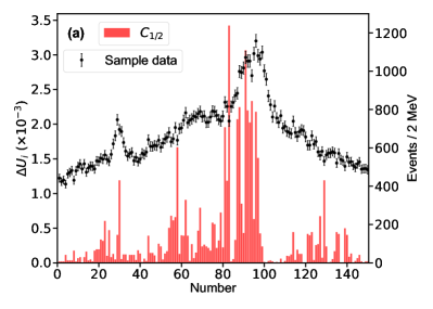
For this purpose, we define the uncertainty for the th parameter of , which is determined with the central values obtained by switching on/off the th bin of in the fitting. The bigger uncertainty observed by excluding a bin means a larger impact power of the bin on a parameter. Fig. 6 illustrates the distributions for two of the eleven parameters. The distributions for other parameters can be found in the Supplementary materials. The bins near the peaks in the mass spectrum do not show stronger constraints on the uncertainties of the parameters and than the others. That is because that the model parameters are correlated to each other and do not reflect the underlying physics directly. In addition, to check the impact of the th experimental point on the pole positions of the channel, the uncertainty
| (20) |
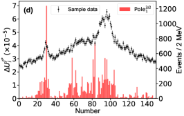
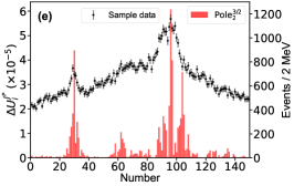
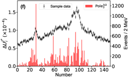
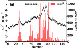
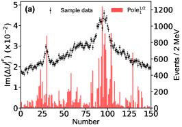
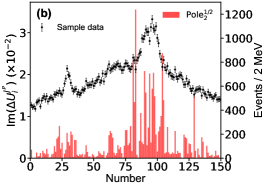
for the real part of the th pole position is defined by switching on/off the th bin of in the fitting. A similar behavior can be found for the imaginary part of the poles, see Supplementary materials. Fig. 7 illustrates the distributions for the and channels, respectively, without considering the correlation among the parameters. Although those values are of the order , one can still see that the experimental data around the , , and thresholds are more important than the others. The reason why the data around the threshold is not important is that the small production amplitude of the channel and the experimental data have little constraint about the corresponding poles [50, 51]. One can also obtain the same conclusion from Fig. 7g, where the experimental data around the dynamic channel do not show any significance. Due to the coupled-channel effect, the experimental data around the coupled channels still have strong constraints on the physics, e.g. the seven poles, around the other coupled channels. Taking the first pole of the channel as an example, e.g. Fig. 7a, the data around the threshold are as significant as those around the threshold. As the sample data of Fig. 7 corresponds to Solution A, the data around () are more important than those around the () in Fig. 7b (Fig. 7e) as expected.
VII Conclusion
We have investigated the nature of the famous hidden charm pentaquarks with a NN-based approach in a pionless EFT, which strongly favors and , i.e. solution A in Refs [49, 50, 51, 58, 59]. From this NN, we find that solution A is systematically preferred over solution B. This conclusion is based on the pionless EFT, which is used to illustrate the difference between the machine learning and the normal fitting approach. Furthermore, we also performed checks on both the NN-based approach and the /ndf-fitting approach. Our conclusion is that both approaches work well on the MC simulation samples. In the NN-based approach, the role of each data bin on the underlying physics is well reflected by the SHAP value. For the /ndf-fitting approach, such a direct relation does not exist. This further explains why the two solutions can be better distinguished in the NN-based approach than in the /ndf-fitting approach. At the same time, the effect of the background fraction on the accuracy of the network is accurately obtained, which provides a paradigm for NNs to study exotic hadrons by first extracting the background fraction from the data, and then analyzing the physics of the possible states from the data with the network trained from the corresponding background fraction data. This study provides more insights about how the NN-based approach predicts the nature of exotic states from the mass spectrum.
Acknowledgements: We are grateful to Meng-Lin Du, Feng Kun Guo and Christoph Hanhart for the helpful discussion. This work is partly supported by the National Natural Science Foundation of China with Grant No. 12035007, Guangdong Provincial funding with Grant No. 2019QN01X172, Guangdong Major Project of Basic and Applied Basic Research No. 2020B0301030008. Q.W. and U.G.M. are also supported by the NSFC and the Deutsche Forschungsgemeinschaft (DFG, German Research Foundation) through the funds provided to the Sino-German Collaborative Research Center TRR110 “Symmetries and the Emergence of Structure in QCD” (NSFC Grant No. 12070131001, DFG Project-ID 196253076-TRR 110). The work of U.G.M. is further supported by the Chinese Academy of Sciences (CAS) President’s International Fellowship Initiative (PIFI) (Grant No. 2018DM0034) and Volkswagen Stiftung (Grant No. 93562).
Author contributions: Zhenyu Zhang and Jiahao Liu did the calculations. Jifeng Hu, Qian Wang and Ulf-G. Meißner focused on how to use machine learning to solve the problems in hadron physics. All the authors made substantial contributions to the physical and technical discussions as well as the editing of the manuscript. All the authors have read and approved the final version of the manuscript.
References
- [1] LHCb Collaboration, Aaij R, et al. Observation of resonances consistent with pentaquark states in decays. Phys Rev Lett 2015;115:072001.
- [2] LHCb Collaboration, Aaij R, et al. Model-independent evidence for contributions to decays. Phys Rev Lett 2016;117:082002.
- [3] LHCb Collaboration, Aaij R, et al. Observation of a narrow pentaquark state, , and of two-peak structure of the . Phys Rev Lett 2019;122:222001.
- [4] LHCb Collaboration, Aaij R, et al. Observation of structure in the -pair mass spectrum. Sci Bull 2020;65:1983–1993.
- [5] CMS Collaboration. Observation of new structures in the mass spectrum in collisions at TeV. 2022, CMS-PAS-BPH-21-003.
- [6] ATLAS Collaboration. Observation of an excess of di-charmonium events in the four-muon final state with the ATLAS detector. 2022, ATLAS-CONF-2022-040.
- [7] LHCb Collaboration, Aaij R, et al. Observation of an exotic narrow doubly charmed tetraquark. Nat Phys 2022;18:751–754.
- [8] LHCb Collaboration, Aaij R, et al. Study of the doubly charmed tetraquark . Nat Commun 2022;13:3351.
- [9] Chen H-X, Chen W, Liu X, et al. A review of the open charm and open bottom systems. Rept Prog Phys 2017;80:076201.
- [10] Chen H-X, Chen W, Liu X, et al. The hidden-charm pentaquark and tetraquark states. Phys Rept 2016;639:1–121.
- [11] Lebed RF, Mitchell RE, Swanson ES. Heavy-quark QCD exotica. Prog Part Nucl Phys 2017;93:143–194.
- [12] Guo F-K, Christoph H, Meiner Ulf-G, et al. Hadronic molecules. Rev Mod Phys 2018;90:015004.
- [13] Dong Y, Faessler A, Lyubovitskij VE. Description of heavy exotic resonances as molecular states using phenomenological lagrangians. Prog Part Nucl Phys 2017;94:282–310.
- [14] Albuquerque RM, Dias JM, Khemchandani KP, et al. QCD sum rules approach to the and states. J Phys G 2019;46:093002.
- [15] Brambilla N, Eidelman S, Hanhart C, et al. The states: experimental and theoretical status and perspectives. Phys Rept 2020;873:1–154.
- [16] Liu Y-R, Chen H-X, Chen W, et al. Pentaquark and tetraquark states. Prog Part Nucl Phys 2019;107:237–320.
- [17] Guo F-K, Liu X-H, Sakai S. Threshold cusps and triangle singularities in hadronic reactions. Prog Part Nucl Phys 2020;112:103757.
- [18] JPAC Collaboration, Albaladejo M, et al. Novel approaches in hadron spectroscopy. Prog Part Nucl Phys 2022;127:103981.
- [19] Zou B-S. Building up the spectrum of pentaquark states as hadronic molecules. Sci Bull 2021;66:1258.
- [20] Mai M, Meiner U-G, Urbach C. Towards a theory of hadron resonances. Phys Rept 2023;1001:1–66.
- [21] Ng L, Bibrzycki L, Nys J, et al. Deep learning exotic hadrons. Phys Rev D 2022;105:L091501.
- [22] Ireland D G, Janssen S, Ryckebusch J. A genetic algorithm analysis of N∗ resonances in reactions. Nucl Phys A 2004;740:147–167.
- [23] Fernández-Ramírez C, de Guerra EM, Udías A, et al. Properties of nucleon resonances by means of a genetic algorithm. Phys Rev C 2008;77:065212.
- [24] The NNPDF collaboration, Ball RD, et al. Parton distributions for the LHC Run II. J High Energy Phys 2015;04:040.
- [25] Forte S, Garrido L, Latorre JI, et al. Neural network parametrization of deep inelastic structure functions. J High Energy Phys 2002;05:062.
- [26] Rojo J, Latorre JI. Neural network parametrization of spectral functions from hadronic tau decays and determination of QCD vacuum condensates. J High Energy Phys 2004;01:055.
- [27] Keeble JWT, Rios A. Machine learning the deuteron. Phys Lett B 2020;809:135743.
- [28] Adams C, Carleo G, Lovato A, et al. Variational Monte Carlo calculations of A4 nuclei with an artificial neural-network correlator ansatz. Phys Rev Lett 2021;127:022502.
- [29] Niu Z-M, Liang H-Z. Nuclear mass predictions based on bayesian neural network approach with pairing and shell effects. Phys Lett B 2018;778:48–53.
- [30] Niu Z-M, Liang H-Z, Sun B-H, et al. Predictions of nuclear -decay half-lives with machine learning and their impact on -process nucleosynthesis. Phys Rev C 2019;99:064307.
- [31] Ma C-W, Peng D, Wei H-L, et al. Isotopic cross-sections in proton induced spallation reactions based on the bayesian neural network method. Chin Phys C 2020;44:014104.
- [32] Kaspschak B, Meiner U-G. How machine learning conquers the unitary limit. Commun Theor Phys 2021;73:035101.
- [33] Kaspschak B, Meiner U-G. Three-body renormalization group limit cycles based on unsupervised feature learning. Mach Learn Sci Tech 2022;3:025003.
- [34] Bedaque P, Boehnlein A, Cromaz M, et al. A.I. for nuclear physics. Eur Phys J A 2021;57:100.
- [35] Dong X-X, An R, Lu J-X, et al. Nuclear charge radii in bayesian neural networks revisited. arXiv:2206.13169, 2022.
- [36] Baldi P, Bauer K, Eng C, et al. Jet substructure classification in high-energy physics with deep neural networks. Phys Rev D 2016;93:094034.
- [37] Baldi P, Sadowski P, Whiteson D. Searching for exotic particles in high-energy physics with deep learning. Nat Commun 2014;5:4308.
- [38] Boehnlein A, Diefenthaler M, Sato N, et al. Colloquium: machine learning in nuclear physics. Rev Mod Phys 2022;94:031003.
- [39] Guest D, Cranmer K, Whiteson D. Deep learning and its application to LHC physics. Annu Rev Nucl Part Sci 2018;68:161–181.
- [40] Whiteson S, Whiteson D. Machine learning for event selection in high energy physics. Eng Appl Artif Intell 2009;22:1203–1217.
- [41] Carleo G, Troyer M, Solving the quantum many-body problem with artificial neural networks. Science 2017;355:602–606.
- [42] Huang H-Y, Kueng R, Torlai G, et al. Provably efficient machine learning for quantum many-body problems. Science 2022;377:eabk3333.
- [43] Lu Y, Wang Y-J, Chen Y, et al. Rediscovery of numerical lüscher’s formula from the neural network. arXiv:2210.02184, 2022.
- [44] Zhang Z, Ma R, Hu J, et al. Approach the gell-mann-okubo formula with machine learning. Chin Phys Lett 2022;39:111201.
- [45] Sombillo DLB, Ikeda Y, Sato T, et al. Model independent analysis of coupled-channel scattering: a deep learning approach. Phys Rev D 2021;104:036001.
- [46] Sombillo DLB, Ikeda Y, Sato T, et al. Unveiling the pole structure of S-matrix using deep learning. Rev Mex Fis Suppl 2022;3:0308067.
- [47] Liu J, Zhang Z, Hu J, et al. Study of exotic hadrons with machine learning. Phys Rev D 2022;105:076013.
- [48] Sombillo DLB, Ikeda Y, Sato T, et al. Classifying the pole of an amplitude using a deep neural network. Phys Rev D 2020;102:016024.
- [49] Liu M-Z, Pan Y-W, Peng F-Z, et al. Emergence of a complete heavy-quark spin symmetry multiplet: seven molecular pentaquarks in light of the latest LHCb analysis. Phys Rev Lett 2019;122:242001.
- [50] Du M-L, Vadim B, Guo F-K, et al. Interpretation of the LHCb states as hadronic molecules and hints of a narrow . Phys Rev Lett 2020;124:072001.
- [51] Du M-L, Vadim B, Guo F-K, et al. Revisiting the nature of the pentaquarks. J High Energy Phys 2021;08:157.
- [52] Voloshin MB. Radiative transitions from to molecular bottomonium. Phys Rev D 2011;84:031502.
- [53] Meiner U-G, Rusetsky A. Effective field theories. Cambridge: Cambridge University Press 2022.
- [54] Brun R, Rademakers F, ROOT: an object oriented data analysis framework. Nucl Instrum Meth A 1997;389:81–86.
- [55] Galassi M, Theiler J, Davies J, et al. GNU scientific library reference manual (3rd Ed.). ISBN 0954612078.
- [56] He K, Zhang X, Ren S, et al. Deep residual learning for image recognition. arXiv:1512.03385, 2015.
- [57] Kingma DP, Ba J. Adam: a method for stochastic optimization. arXiv:1412.6980, 2014.
- [58] Wang B, Meng L, Zhu S-L. Hidden-charm and hidden-bottom molecular pentaquarks in chiral effective field theory. J High Energy Phys 2019;11:108.
- [59] Yang Z-C, Sun Z-F, He J, et al. The possible hidden-charm molecular baryons composed of anti-charmed meson and charmed baryon. Chin Phys C 2012;36:6–13.
- [60] Murtagh F. Multilayer perceptrons for classification and regression. Neurocomputing 1991;2:183.
- [61] Paszke A, Gross S, Massa F, et al. Pytorch: an imperative style, high-performance deep learning library. arXiv:1912.01703, 2019.
- [62] Clavijo JM, Glaysher P, Jitsev J, et al. Adversarial domain adaptation to reduce sample bias of a high energy physics event classifier. Mach learn: sci technol 2021;3:015014.
Supplemental Material for “Revealing the nature of hidden charm pentaquarks with machine learning”
Appendix A Fitting to the Background Distributions
The background, see Fig. 8, is described by sixth-order Chebyshev polynomials (22), with the coefficients listed in Tab. 3, by fitting the experimental background. The template recursive functions (21) for defining the Chebyshev polynomials is,
| (21) | |||
This allows for the implementation of the Chebyshev polynomials as
| (22) | |||
where the are coefficients, as given in Tab. 3 for the problem at hand.
| Coefficients | Value | Error |
|---|---|---|
| 67.96 | 0.18 | |
| 4.13 | 0.18 | |
| 16.60 | 0.15 | |
| 2.55 | 0.15 | |
| 3.27 | 0.14 | |
| 2.88 | 0.14 | |
| 1.66 | 0.14 |
Appendix B Determination of the Background Fraction in Data
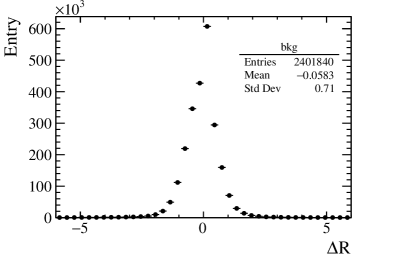
We produce a group of samples for different background fractions from 0% to 90% every 10%, as well as (92%, 94%, 96%). We trained a ResNet-based NN which employs the MSELoss function to measure the Euclidean distance between the predicted background fractions and the truth values. The NN successfully retrieves the background fraction, as illustrated in Fig. 9 (left). The right plot shows the difference between the predicated values and the background values. The bias and uncertainty values are -0.0583 and 0.71, respectively. We then use this NN to determine the background fraction for experimental data. The background fraction for data is determined to be )% in case of training the NN with samples , and is determined to be % in case of training the NN with samples . The background fraction is determined to be % predicted with a different training. In short, the background fraction is taken as their average value .
Appendix C The impact of the energy bins on the model parameters
We define the uncertainty
| (23) |
for the th parameter of , which is determined with the central values obtained by switching on/off the th bin of in the fitting. We use to measure the influence of each data point on a parameter. Figure 10 illustrates distributions w.r.t eleven parameters. The larger points correspond to data points deviating strongly from the interpolation of its neighbour data points.
Appendix D The impact of the energy bins on the imaginary part of the pole positions.
We define the uncertainty
| (24) |
for the imaginary part of the th pole position by switching on/off the th bin of in the fitting. Figs. 11, 12, 13 illustrates the distributions for the channels, respectively, without considering the correlation among the parameters.


Appendix E Detailed Predictions
To reduce the systematic uncertainties arising from the NNs, we trained several NN models with identical structure but different initializations. In particular, for the background fractions , , , and , we train ten NNs, respectively. Their predicted results are presented in Tab. 4 with maximum probabilities in boldface. As shown in the table, the first labels of all the maximum probabilities are “1”, which indicates that all the NNs favor solution A, i.e. and . As these 40 NNs can distinguish solution A from solution B.
| Label | |||||||||||||||
| 0000 | 1000 | 1001 | 1002 | 0100 | 0110 | 0111 | 1111 | 0200 | 1200 | 1210 | 1211 | 1220 | 1221 | 1222 | |
| Prediction of NN trained with samples at a background level 90%. | |||||||||||||||
| NN 1 (77.29%) | 0.69 | 89.13 | 1.42 | 8.75 | 0.00 | 0.00 | 0.00 | 0.00 | 0.00 | 0.00 | 0.00 | 0.00 | 0.00 | 0.01 | 0.00 |
| NN 2 (74.64%) | 0.03 | 5.83 | 38.47 | 55.30 | 0.00 | 0.03 | 0.08 | 0.00 | 0.07 | 0.04 | 0.02 | 0.00 | 0.00 | 0.09 | 0.04 |
| NN 3 (74.97%) | 0.03 | 5.39 | 15.79 | 78.41 | 0.00 | 0.02 | 0.03 | 0.00 | 0.00 | 0.00 | 0.00 | 0.00 | 0.00 | 0.03 | 0.03 |
| NN 4 (75.94%) | 0.01 | 1.90 | 27.01 | 70.95 | 0.00 | 0.01 | 0.01 | 0.00 | 0.00 | 0.01 | 0.00 | 0.00 | 0.01 | 0.03 | 0.06 |
| NN 5 (74.07%) | 2.40 | 94.45 | 0.15 | 2.99 | 0.00 | 0.00 | 0.00 | 0.00 | 0.00 | 0.00 | 0.00 | 0.00 | 0.00 | 0.01 | 0.00 |
| NN 6 (77.56%) | 0.05 | 2.76 | 31.64 | 65.36 | 0.00 | 0.01 | 0.03 | 0.00 | 0.00 | 0.02 | 0.00 | 0.00 | 0.01 | 0.02 | 0.08 |
| NN 7 (76.79%) | 0.11 | 4.16 | 35.17 | 60.23 | 0.00 | 0.04 | 0.06 | 0.00 | 0.01 | 0.04 | 0.00 | 0.00 | 0.00 | 0.04 | 0.13 |
| NN 8 (76.78%) | 0.18 | 4.23 | 16.10 | 79.44 | 0.00 | 0.00 | 0.00 | 0.00 | 0.00 | 0.00 | 0.00 | 0.00 | 0.00 | 0.02 | 0.02 |
| NN 9 (75.22%) | 0.11 | 2.54 | 18.26 | 79.02 | 0.00 | 0.00 | 0.02 | 0.00 | 0.00 | 0.00 | 0.00 | 0.00 | 0.00 | 0.03 | 0.01 |
| NN 10 (75.87%) | 0.00 | 1.24 | 22.85 | 75.77 | 0.00 | 0.00 | 0.02 | 0.00 | 0.00 | 0.00 | 0.00 | 0.00 | 0.00 | 0.00 | 0.09 |
| Prediction of NN trained with samples at a background level 92%. | |||||||||||||||
| NN 1 (72.94%) | 0.00 | 0.15 | 5.37 | 94.47 | 0.00 | 0.00 | 0.00 | 0.00 | 0.00 | 0.00 | 0.00 | 0.00 | 0.00 | 0.00 | 0.00 |
| NN 2 (72.68%) | 0.00 | 0.07 | 4.11 | 95.81 | 0.00 | 0.00 | 0.00 | 0.00 | 0.00 | 0.00 | 0.00 | 0.00 | 0.00 | 0.00 | 0.00 |
| NN 3 (74.58%) | 0.00 | 0.78 | 13.57 | 85.61 | 0.00 | 0.00 | 0.01 | 0.00 | 0.00 | 0.00 | 0.00 | 0.00 | 0.00 | 0.00 | 0.02 |
| NN 4 (71.78%) | 0.00 | 0.81 | 19.02 | 80.16 | 0.00 | 0.00 | 0.00 | 0.00 | 0.00 | 0.00 | 0.00 | 0.00 | 0.00 | 0.00 | 0.00 |
| NN 5 (72.75%) | 0.14 | 15.13 | 16.91 | 67.80 | 0.00 | 0.00 | 0.00 | 0.00 | 0.00 | 0.00 | 0.00 | 0.00 | 0.00 | 0.00 | 0.00 |
| NN 6 (71.72%) | 0.00 | 0.18 | 9.32 | 90.48 | 0.00 | 0.00 | 0.00 | 0.00 | 0.00 | 0.00 | 0.00 | 0.00 | 0.00 | 0.00 | 0.00 |
| NN 7 (72.75%) | 0.00 | 0.32 | 18.44 | 81.24 | 0.00 | 0.00 | 0.00 | 0.00 | 0.00 | 0.00 | 0.00 | 0.00 | 0.00 | 0.00 | 0.00 |
| NN 8 (74.57%) | 0.00 | 0.27 | 6.39 | 93.34 | 0.00 | 0.00 | 0.00 | 0.00 | 0.00 | 0.00 | 0.00 | 0.00 | 0.00 | 0.00 | 0.00 |
| NN 9 (73.24%) | 0.00 | 0.00 | 1.05 | 98.95 | 0.00 | 0.00 | 0.00 | 0.00 | 0.00 | 0.00 | 0.00 | 0.00 | 0.00 | 0.00 | 0.00 |
| NN 10 (74.34%) | 0.00 | 0.02 | 0.85 | 99.12 | 0.00 | 0.00 | 0.00 | 0.00 | 0.00 | 0.00 | 0.00 | 0.00 | 0.00 | 0.00 | 0.00 |
| Prediction of NN trained with samples at a background level 94%. | |||||||||||||||
| NN 1 (65.28%) | 0.00 | 1.20 | 2.26 | 96.53 | 0.00 | 0.00 | 0.00 | 0.00 | 0.00 | 0.00 | 0.00 | 0.00 | 0.00 | 0.00 | 0.00 |
| NN 2 (64.11%) | 0.02 | 2.23 | 11.51 | 86.24 | 0.00 | 0.00 | 0.00 | 0.00 | 0.00 | 0.00 | 0.00 | 0.00 | 0.00 | 0.00 | 0.00 |
| NN 3 (67.83%) | 0.00 | 0.26 | 10.26 | 89.47 | 0.00 | 0.00 | 0.00 | 0.00 | 0.00 | 0.00 | 0.00 | 0.00 | 0.00 | 0.00 | 0.00 |
| NN 4 (65.53%) | 0.15 | 24.05 | 48.79 | 26.89 | 0.00 | 0.04 | 0.02 | 0.00 | 0.01 | 0.03 | 0.00 | 0.00 | 0.00 | 0.02 | 0.01 |
| NN 5 (64.17%) | 0.02 | 4.12 | 72.61 | 23.23 | 0.00 | 0.00 | 0.01 | 0.00 | 0.00 | 0.00 | 0.00 | 0.00 | 0.00 | 0.01 | 0.00 |
| NN 6 (67.44%) | 0.00 | 1.22 | 13.92 | 84.86 | 0.00 | 0.00 | 0.00 | 0.00 | 0.00 | 0.00 | 0.00 | 0.00 | 0.00 | 0.00 | 0.00 |
| NN 7 (61.85%) | 0.00 | 5.07 | 15.90 | 79.01 | 0.00 | 0.00 | 0.00 | 0.00 | 0.00 | 0.00 | 0.00 | 0.00 | 0.00 | 0.00 | 0.00 |
| NN 8 (65.73%) | 0.03 | 1.31 | 58.42 | 40.21 | 0.00 | 0.00 | 0.02 | 0.00 | 0.00 | 0.00 | 0.00 | 0.00 | 0.00 | 0.00 | 0.00 |
| NN 9 (65.34%) | 0.00 | 2.94 | 21.80 | 75.25 | 0.00 | 0.00 | 0.00 | 0.00 | 0.00 | 0.00 | 0.00 | 0.00 | 0.00 | 0.00 | 0.01 |
| NN 10 (65.74%) | 0.00 | 0.08 | 4.56 | 95.34 | 0.00 | 0.00 | 0.00 | 0.00 | 0.00 | 0.00 | 0.00 | 0.00 | 0.00 | 0.00 | 0.00 |
| Prediction of NN trained with samples at a background level 96%. | |||||||||||||||
| NN 1 (55.64%) | 0.00 | 1.29 | 19.79 | 78.92 | 0.00 | 0.00 | 0.00 | 0.00 | 0.00 | 0.00 | 0.00 | 0.00 | 0.00 | 0.00 | 0.00 |
| NN 2 (54.75%) | 0.00 | 3.38 | 25.64 | 70.97 | 0.01 | 0.00 | 0.00 | 0.00 | 0.00 | 0.00 | 0.00 | 0.00 | 0.00 | 0.00 | 0.00 |
| NN 3 (53.44%) | 0.00 | 6.57 | 32.20 | 61.23 | 0.00 | 0.00 | 0.00 | 0.00 | 0.00 | 0.00 | 0.00 | 0.00 | 0.00 | 0.00 | 0.00 |
| NN 4 (51.20%) | 0.60 | 55.77 | 21.65 | 21.96 | 0.00 | 0.00 | 0.00 | 0.00 | 0.00 | 0.00 | 0.00 | 0.00 | 0.00 | 0.00 | 0.00 |
| NN 5 (56.41%) | 0.00 | 0.27 | 3.52 | 96.20 | 0.00 | 0.00 | 0.00 | 0.00 | 0.00 | 0.00 | 0.00 | 0.00 | 0.00 | 0.00 | 0.00 |
| NN 6 (50.72%) | 0.39 | 34.89 | 31.27 | 33.42 | 0.00 | 0.00 | 0.00 | 0.00 | 0.00 | 0.00 | 0.00 | 0.00 | 0.00 | 0.00 | 0.00 |
| NN 7 (54.34%) | 0.00 | 5.16 | 21.02 | 73.82 | 0.00 | 0.00 | 0.00 | 0.00 | 0.00 | 0.00 | 0.00 | 0.00 | 0.00 | 0.00 | 0.00 |
| NN 8 (53.04%) | 0.02 | 5.04 | 33.86 | 61.08 | 0.00 | 0.00 | 0.00 | 0.00 | 0.00 | 0.00 | 0.00 | 0.00 | 0.00 | 0.00 | 0.00 |
| NN 9 (58.18%) | 0.00 | 0.11 | 31.92 | 67.97 | 0.00 | 0.00 | 0.00 | 0.00 | 0.00 | 0.00 | 0.00 | 0.00 | 0.00 | 0.00 | 0.00 |
| NN 10 (55.79%) | 0.05 | 18.82 | 28.80 | 52.32 | 0.00 | 0.00 | 0.00 | 0.00 | 0.00 | 0.00 | 0.00 | 0.00 | 0.00 | 0.00 | 0.00 |
Appendix F Neural Network
We have compared a MLP-based [60] NN to a ResNet-based [56] NN, which are implemented using PyTorch [61]. Both NN models are trained with the samples. The Adam [57] optimizer is used to solve these models with a combination of the momentum algorithm with the RMSProp algorithm [62]. For the activation function, the Relu function compared to the Sigmod function, can effectively avoid the problem of gradient disappearance and alleviate potential overfitting in particular when training a deep neutral network, while the Sigmod function is exponential and computationally expensive. A reasonable solution can be obtained after 500 training epochs using an initial learning rate value of 0.001. A large learning rate makes convergence of the loss function difficult, while a small learning rate makes too slow convergence. Our strategy is to dynamically reduce it. The initial learning rate of 0.001 is successfully tested, and the next interval is reduced to the of the previous one, controlled by the stepLR method. The interval is set to 100 epochs in our case. To avoid the network falling into the local minimum solution during the training process, the weights of the neurons are randomly initialized with a normal distribution, and the biases of neurons are set to zero.
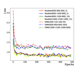
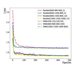
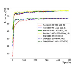
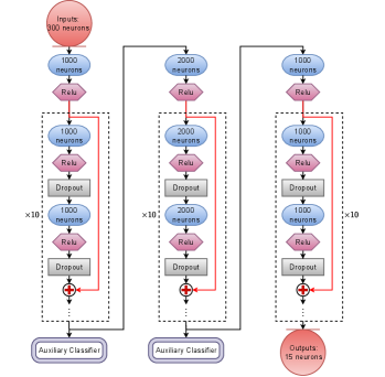
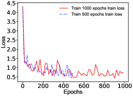
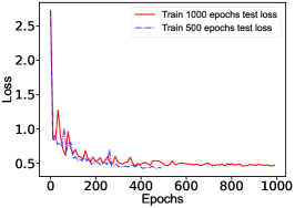
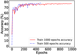
To avoid overfitting in the training, we introduce dropout layers in the network. A large dropout probability tends to activate too few neurons and the loss function will not converge; a small dropout probability tends to reduce generalizability and even occur over-fitting. After training, the dropout probability is chosen to 0.3 for ResNet-based NN and 0.2 for MLP-based NN to optimize performance. In case of overfiting, the obtained NN works well on training datasets while probably does not on testing datasets. Thus the loss function calculated with training datasets should obviously differs from the one calculated with testing datasets. However, one cannot see difference in Fig. 16, which indicates the NN works well both for training and testing datasets. In summary, the CrossEntropyLoss function converges as the training epochs increase, and the predicted accuracy increases as training epochs increase. The ResNet-based NN achieves a better solution, as shown in Fig. 14. A larger number of neurons and hidden layers require more computing resources and result in difficult training and over-fitting; while a smaller number of neurons and hidden layers result in non-convergence of the loss function and under-fitting. We found an architecture ResNet(1000-1000-2000-2000-1000-1000_10) which works well after several attempts without optimizing its architecture. The ResNet-based NN is structured as shown in Fig. 15.
Appendix G What is the reason for the saturation of NN’s accuracy?
The low accuracy is because of two reasons,
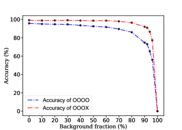
(1) Background fraction. Higher background fractions imply lower prediction accuracy within our expectation. Clearly at an extreme case 100% background fraction will result in a zero accuracy. To make this point clear, we study how the prediction accuracy varies with background fractions, with lots of samples (, , , , , , , , , , , , ), as summarized in the Tab. 5 (1st and 2nd column), and Fig. 17 (left).
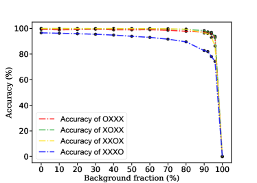
(2) The forth label, since the peak corresponding to the forth label is submerged in background, the NN fails to predict this label. Thus when we count correct predictions including this label “OOOO” (2nd column), the accuracy drops down. In turn, when we count correct predictions excluding this label “OOOX” (3rd column), the accuracy goes up. Please see also Fig. 17. We also show the more results (accuracy of “OXXX”, “XOXX”, “XXOX”, “XXXO”) in Fig. 17 (right), and find that the accuracy of “XXXO” is the lowest.
| Background fraction | Accuracy of “OOOO”(%) | Accuracy of “OOOX”(%) |
|---|---|---|
| 95.70 | 99.14 | |
| 95.03 | 98.80 | |
| 94.73 | 98.86 | |
| 94.56 | 99.10 | |
| 93.52 | 98.74 | |
| 92.49 | 98.60 | |
| 91.70 | 98.70 | |
| 89.52 | 97.91 | |
| 85.99 | 96.45 | |
| 74.70 | 91.93 | |
| 73.11 | 90.90 | |
| 65.30 | 86.62 | |
| 56.02 | 77.30 |
Appendix H SHAP Value
The SHapley Additive exPlanation (SHAP) value is widely used as a feature importance metric for well-established models in machine learning. One of prevailing methods for estimating neural network model features is the DeepLIFT algorithm based DeepExplainer. A positive (negative) SHAP value indicates that a given data point is pushing the NN classification in favor of (against) a given class. A large absolute SHAP value implies a large impact of a given mass bin on the classification. The method requires a dataset as a reference (or denoted as background) for evaluating network features, and we test the SHAP values of 1000 {} samples and the SHAP values of experimental data with our network based on 3000 {} samples as a reference. Fig.18 shows the SHAP values of experimental data corresponding to 15 labels, indicating that data points around the peaks in the mass spectrum have a greater impact. Fig. 19 shows the SHAP values of MC samples corresponding to 15 labels.