Revenue Comparisons of Auctions
with Ambiguity Averse Sellers
Abstract
We study the revenue comparison problem of auctions when the seller has a maxmin expected utility preference. The seller holds a set of priors around some reference belief, interpreted as an approximating model of the true probability law or the focal point distribution. We develop a methodology for comparing the revenue performances of auctions: the seller prefers auction to auction if their transfer functions satisfy a weak form of the single-crossing condition. Intuitively, this condition means that a bidder’s payment is more negatively associated with the competitor’s type in than in . Applying this methodology, we show that when the reference belief is independent and identically distributed (IID) and the bidders are ambiguity neutral, (i) the first-price auction outperforms the second-price and all-pay auctions, and (ii) the second-price and all-pay auctions outperform the war of attrition. Our methodology yields results opposite to those of the Linkage Principle.
keywords:
Auctions; Ambiguity; Revenue comparison. JEL Classification Numbers: D44, D81, D82.1 Introduction
Since the establishment of the Revenue Equivalence Principle (Myerson, 1981), an important problem of auction theory is to compare the revenue performances of different auctions in setups relaxing Myerson’s (1981) standard assumptions. The Linkage Principle (Milgrom and Weber, 1982; Krishna and Morgan, 1997), one of the fundamental results in this direction, states that in the affiliated interdependent values setup, auctions with stronger positive linkages between a bidder’s payment and her own signal yield higher expected revenues. Succeeding works study the effects of the bidders’ risk aversion (Maskin and Riley, 1984), the seller’s risk aversion (Waehrer et al., 1998), the bidders’ financial constraints (Che and Gale, 1998), and asymmetric valuation distributions (Maskin and Riley, 2000).
This paper studies the revenue comparison problem in which the seller’s preference exhibits ambiguity aversion (Ellsberg, 1961). One of our main contributions, Theorem 2, provides a methodology to compare the revenue performances of different auctions. Intuitively, it states that auctions in which a bidder’s payment is more negatively associated with the competitor’s type yield higher revenues. Applying this methodology, we compare the revenues of four commonly studied auctions: the first-price, second-price, all-pay auctions and war of attrition.
Following the maxmin expected utility model (MMEU; Gilboa and Schmeidler, 1989), the seller holds a set of priors around some reference belief and evaluates an auction by the worst-case revenue, the minimum expected revenue over the set of priors. The reference belief can be interpreted as an approximation of the true distribution (Hansen and Sargent, 2001, 2008) or the focal point distribution (Bose et al., 2006; Bose and Daripa, 2009). To present our results clearly, we focus primarily on the case of ambiguity neutral bidders; however, most of our results extend to the case of ambiguity averse bidders (Section 6.1).
To develop our main methodology, we first show that in finding the beliefs that minimize the seller’s expected revenue, we can restrict attention to a special class of beliefs within the set of priors named the decreasing rearrangements (Theorem 1). A rearrangement of a belief reassigns probabilities over the state space; it is called a decreasing rearrangement if it overweights the likelihood of low types and underweights that of high types relative to the reference belief (Definition 1). Since facing low types is an unfavorable event and facing high types is a favorable event for the seller, Theorem 1 is intuitive. To confirm this intuition, for a given belief, we explicitly construct its decreasing rearrangement that yields a lower expected revenue than the original belief. To ensure that this decreasing rearrangement lies in the set of priors, we assume that the set of priors is rearrangement invariant, i.e., it is closed under the rearrangement operation (Assumptions 1A-1B). This assumption is satisfied by a wide range of sets of priors used in the literature—most importantly, the relative entropy neighborhood (Example 1; Hansen and Sargent, 2001, 2008).
Building on Theorem 1, Theorem 2 states that the seller prefers auction to auction if the following two conditions hold. First, each type of bidder’s payment is greater (or smaller) in than in against a competitor with low types (or high types) (Weak Single-Crossing Condition, WSCC; Figure 3). This condition is a weak form of the standard single-crossing condition (SCC) in auction theory (Milgrom, 2004); hence the name WSCC. Intuitively, WSCC means that a bidder’s payment is more negatively associated with the competitor’s type in than in . Second, yields at least as high interim expected revenues as under the reference belief (Reference Revenue Condition, RRC). In applications, the second condition automatically holds as equality by the Revenue Equivalence Principle (Myerson, 1981). Thus, Theorem 2 shows that auctions with stronger negative associations between a bidder’s payment and her competitor’s type yield higher worst-case revenues.
The intuition behind Theorem 2 is as follows. By WSCC, a bidder’s payment is greater (or smaller) in than in against a competitor with low types (or high types). However, a decreasing rearrangement overweights the likelihood of low types and underweights that of high types relative to the reference belief. Hence, it overweights the event that the bidder’s payment is greater in than in , and underweights the opposite event. This, together with RRC, implies that under any decreasing rearrangement, yields a higher expected revenue than . By Theorem 1, the worst-case revenue—the minimum over the decreasing rearrangements within the set of priors—is higher in than in .
Then, applying Theorem 2, we establish the worst-case revenue rankings between the four commonly studied auctions (Theorem 3 and Figures 5-6). We find that when the reference belief is independent and identically distributed (IID) and the bidders are ambiguity neutral, (i) the first-price auction outperforms the second-price and all-pay auctions, and (ii) the second-price and all-pay auctions outperform the war of attrition. The ranking between the second-price and all-pay auctions is indeterminate (Figure 7).
Notably, the worst-case revenue rankings in Theorem 3 are opposite to the expected revenue rankings in the affiliated values setup (Milgrom and Weber, 1982; Krishna and Morgan, 1997). This is because Theorem 2 works in the opposite direction to the Linkage Principle (Proposition 1). Recall that according to Theorem 2, if a bidder’s payment is more negatively associated with the competitor’s type in auction than in auction (WSCC), then outperforms . By contrast, the Linkage Principle states that if a bidder’s payment is more negatively associated with her own type in than in (Linkage Condition, LC; Theorem 4), then outperforms . However, a negative association between a bidder’s payment and her competitor’s type creates a negative association between her payment and her own type in the affiliated values setup. As a result, WSCC and LC hold simultaneously, and thus the two principles predict opposite results. This logic also implies that in the presence of both ambiguity and affiliation, the rankings between the four auctions are indeterminate (Figure 8).
Our paper is related to Che and Gale (1998) in that a version of the single-crossing condition determines the revenue ranking between auctions. Specifically, Che and Gale (1998) study the setup in which each bidder has private information about her valuation and budget. They show that if the iso-bid curves of two auctions in the two-dimensional space of valuation and budget satisfy a single-crossing condition, their revenues can be compared. Waehrer et al. (1998) also analyze the setup where the seller is risk averse, a natural benchmark for our study. They show that the first-price auction outperforms the second-price auction because the winner’s payment is less variable (in the sense of second-order stochastic dominance) in the first-price auction than in the second-price auction. However, their result relies on the assumption that the loser pays nothing, which is violated in the all-pay auction and war of attrition.
The remainder of this paper is organized as follows. Section 2 presents our setup. Section 3 develops our main methodology. As an application, Section 4 compares the four commonly studied auctions. Section 5 discusses the relationship between our methodology and the Linkage Principle. Section 6 provides two extensions: ambiguity averse bidders and ambiguity seeking seller. Section 7 discusses the related literature and concludes the paper.
2 Model
2.1 Agents and preferences
A seller wants to sell an indivisible object to two bidders, denoted by bidders and . Each bidder has a privately known type representing her valuation for the object. There is a commonly known reference belief , a probability measure on . As mentioned in the introduction, can be interpreted as an approximation of the true probability law (Hansen and Sargent, 2001, 2008) or the focal point distribution (Bose et al., 2006; Bose and Daripa, 2009). Assume has a positive probability density.
The seller, being ambiguity averse, takes into account the possibility that the true probability law differs from the reference belief. Specifically, she holds a set of priors about the joint type distribution around the reference belief, where . For technical reasons, assume is weakly compact. As mentioned in the introduction, we focus primarily on the case of ambiguity neutral bidders, in which the bidders believe that types are drawn according to the reference belief . The case of ambiguity averse bidders is discussed in Section 6.1.
For a given auction, let denote bidder ’s payment when her type is and her competitor’s type is . We call the transfer function. Following the MMEU model (Gilboa and Schmeidler, 1989), the seller evaluates an auction by the worst-case revenue , the minimum expected revenue over the set of priors:
2.2 Rearrangement
In this section, we first explain the concepts related to rearrangement, and then describe our assumption on the seller’s set of priors named rearrangement invariance. To this end, consider a probability space . Let be the set of all probability measures over that are absolutely continuous with respect to . We introduce the following definition:
Definition 1.
Let .
(i) We say is a rearrangement of (with respect to ) if
| (1) |
(ii) Suppose is endowed with a partial order . We say is a decreasing rearrangement of (with respect to ) if is a rearrangement of , and
| (2) |
Whenever is a product space, is assumed to be the componentwise order. In this case, condition (2) means that decreases in each argument.222Throughout this paper, “increasing” means “non-decreasing” and “decreasing” means “non-increasing”.
(iii) For , we say is rearrangement invariant relative to (with respect to ) if whenever a belief belongs to , its rearrangements in belong to : i.e.,
In particular, if , we simply say is rearrangement invariant.
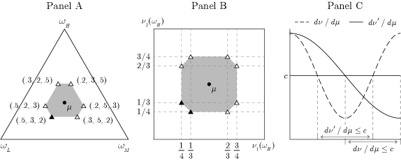
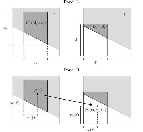
Panel A: Discrete states, the domain of all beliefs. Let (where ), be uniform on , and . A belief is represented by point on the simplex. Each has rearrangements, marked by triangles. Among them, the black triangle is the decreasing rearrangement. The shaded hexagon is rearrangement invariant.
Panel B: Discrete states, the domain of independent beliefs. Let (where ), be uniform on , and be the set of independent beliefs on . A belief is represented by point , where denotes the -th marginal probability measure of . Each has rearrangements; out of these, beliefs marked by triangles are independent, i.e., lie in . Among them, the two black triangles are the decreasing rearrangements. The shaded octagon is rearrangement invariant relative to .
Panel C: Continuous states. Let and be uniform over . Suppose that the Radon-Nikodym derivatives of are given as in the figure. Since the lower contour sets of and have the same length, condition (1) holds. Because is decreasing, is a decreasing rearrangement of .
Figure 1 illustrates Definition 1. To explain Definition 1, consider the simple case of discrete and uniform . Then, the rearrangements are equivalent to the permutations of probabilities over states (Panels A-B, triangles). Among them, the decreasing rearrangements are the permutations that assign high probabilities to low states and low probabilities to high states (Panels A-B, black triangles). Accordingly, rearrangement invariance requires that a set of priors remains unchanged under permutations (Panels A-B, shaded regions). This means that the set of priors—and hence the degree of ambiguity it represents—is independent of the specific ordering of states. Definition 1 extends these concepts to general state spaces (including continuous spaces; Panel C).
One of our main results in Section 3 states that when the set of priors is rearrangement invariant, in finding the beliefs that minimize the seller’s expected revenue, it suffices to focus on the decreasing rearrangements within the set of priors (Theorem 1). To prove this result, for a given belief in the set of priors, we construct its decreasing rearrangement which yields a lower expected revenue than the original belief. The rearrangement invariance property ensures that this decreasing rearrangement lies in the set of priors.
The rearrangement invariance in Definition 1 is also closely related to a property known as probabilistic sophistication (Machina and Schmeidler, 1992; Ghirardato and Marinacci, 2002; Maccheroni et al., 2006; Cerreia-Vioglio et al., 2011, 2012).333This property is also called the neutrality axiom in the literature on probabilistic risk aversion (Yaari, 1987; Safra and Segal, 1998). An MMEU decision maker with a set of priors is said to be probabilistically sophisticated if the following holds: for all bounded measurable functions ,
| (3) | |||
| (4) |
That is, if two acts and have the same outcome distribution under the reference belief , the decision maker is indifferent between them.
Maccheroni et al. (2006, Thm. 14) show that is rearrangement invariant if and only if the decision maker is probabilistically sophisticated. To illustrate the “only if” direction, suppose again that is discrete and is uniform, and let be rearrangement invariant. It can be shown that if two acts and satisfy condition (3), then is a permutation of . This implies that the minimum expectation of over can be expressed as that of over a permutation of . By rearrangement invariance, the permutation of coincides with , establishing equation (4).444More precisely, condition (3) implies that there exists a permutation over satisfying . Then, it can be shown that , where . Rearrangement invariance implies , establishing equation (4). Hence, the decision maker is probabilistically sophisticated.
Now, returning to the auction setup, consider three domains of beliefs :
where denotes the -th marginal probability measure of . Observe that .
Our first assumption on the seller’s set of priors is as follows:
Assumption 1A.
For , the following holds:
(i) .
(ii) is rearrangement invariant with respect to .
This assumption holds for a wide range of sets of priors used in the literature, as shown in Example 1.
Example 1 (Set of priors).
The -divergence is a measure of discrepancy between probability measures used in information theory and statistics (Ali and Silvey, 1966). Given a convex function , the -divergence is defined as follows: for probability measures and on the same state space,
In the special case of , -divergence becomes the popular relative entropy (Kullback and Leibler, 1951).
Now, let be the set of beliefs that are close to the reference belief, where the “closeness” is measured by divergence:
Here, the parameter represents the degree of ambiguity. Maccheroni et al. (2006, Thm. 14 and Lem. 15) show that satisfies Assumption 1A. This is one of the most popular ambiguity sets in the robustness literature (Hansen and Sargent, 2001, 2008; Ben-Tal et al., 2013).
Let be the set of beliefs whose likelihood ratios lie in a given interval:
where represents the degree of ambiguity and . Because the rearrangement operation preserves the range of , satisfies Assumption 1A. In the limiting case of , reduces to the contamination model:
where is normalized to . This model is widely used in the literature on mechanism design with ambiguity (Bose et al., 2006; Bose and Daripa, 2009).
Some studies suppose that the set of priors consists only of independent beliefs or of IID beliefs (e.g., Lo, 1998; Bose et al., 2006). This corresponds to situations in which the seller has additional information that types are independent or IID. In these cases, because a rearrangement of an independent (or IID) belief is not necessarily independent (or IID), Assumption 1A does not hold. To address this issue, we assume that the set of priors is rearrangement invariant relative to the domain of independent beliefs, or to the domain of IID beliefs.
Assumption 1B.
For , the following holds:
(i) .
(ii) is rearrrangement invariant relative to .
We provide two examples that satisfy Assumption 1B.
3 Main results
This section develops a methodology to compare worst-case revenues. Assumption 2 is a common property of most standard auctions:
Assumption 2.
(i) The total transfer increases in each argument.
(ii) The probability measure induced by the total transfer from is atomless: i.e.,
Theorem 1 states that for an auction satisfying Assumption 2, the seller’s worst-case revenue equals the minimum expected revenue over the decreasing rearrangements within the set of priors. Thus, in finding the beliefs that minimize the seller’s expected revenue, we can restrict attention to the decreasing rearrangements.
Theorem 1.
Proof.
See Section 3.1. ∎
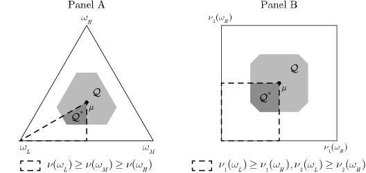
Figure 2 illustrates the set of decreasing rearrangements . Equivalently, can be expressed as the set of beliefs with decreasing likelihood ratios :
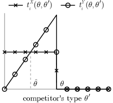
Building on Theorem 1, Theorem 2 states that the seller prefers auction to auction if two conditions hold. First, given and , there exists a threshold such that bidder of type pays a greater (or smaller) amount in than in against a competitor of type (or ) (Weak Single-Crossing Condition, WSCC; Figure 3). This means that a bidder’s payment is more negatively associated with the competitor’s type in than in . Second, under the reference belief, yields at least as high interim expected revenues as (Reference Revenue Condition, RRC). In later applications, this condition automatically holds as an equality by the Revenue Equivalence Principle (Myerson, 1981). Thus, Theorem 2 shows that a negative association between a bidder’s payment and her competitor’s type increases worst-case revenue.
Theorem 2.
Suppose satisfies Assumption 1A or 1B. Let and be auctions whose transfers and satisfy Assumption 2. Assume the following conditions:
(i) Weak Single-Crossing Condition (WSCC). For all and , there exists a threshold such that
(ii) Reference Revenue Condition (RRC). For all and ,
where is the conditional distribution of bidder ’s type given bidder ’s type .555For notational simplicity, we omit the dependence of the conditional distribution on .
Then,
Proof.
See Appendix B. ∎
The intuition of Theorem 2 is as follows. To prove this theorem, we establish the following inequality: for all , and ,
| (5) |
which implies
Then, by Theorem 1, generates a higher worst-case revenue than . To show inequality (5), let be given. By WSCC, bidder of type pays a greater (or smaller) amount in than in against a competitor with low types (or high types). However, a decreasing rearrangement overweights the likelihood of low types and underweights that of high types relative to . Thus, overweights the event that the bidder’s payment is greater in than in , and underweights the opposite event. Because yields at least as high interim expected revenues as under by RRC, yields higher interim expected revenues than under . This establishes the desired inequality (5).
As mentioned in the introduction, WSCC is a weak form of the single-crossing condition familiar from auction theory (Milgrom, 2004, Ch. 4). Recall that and satisfy the single-crossing condition (SCC) if for all , and ,
| (6) |
The first line means that if lies weakly below at some point , then the same holds at every higher point ; the second line is interpreted similarly. Now, WSCC turns out to be equivalent to the following condition (Appendix C): for all , and ,
| (7) |
This means that if lies strictly below at some point , then lies weakly below at every higher point . It is evident that condition (7) is implied by condition (6); hence the name WSCC. Figure 3 illustrates an example that satisfies WSCC but not SCC.666Panels B and C of Figure 6 illustrate examples satisfying SCC. Also, Panel D of Figure 6 illustrates another example satisfying WSCC but not SCC. Like SCC, WSCC requires that crosses at most once and from above (the point ). However, WSCC is weaker than SCC in that it allows the two transfer functions to touch outside the crossing point (the interval ).
3.1 Proof of Theorem 1
This section presents the proof of Theorem 1. We first consider the case of Assumption 1A, and then Assumption 1B.
Case A: satisfies Assumption 1A. To prove Theorem 1, we use Proposition 1, a variant of the Hardy-Littlewood rearrangement inequality (Hardy et al., 1959). Although its proof mostly relies on existing literature (e.g., Luxemburg, 1967; Föllmer and Schied, 2016), we include the proof for completeness.
Proposition 1.
Let be measurable and . Suppose
| (8) |
(i) There exists a rearrangement of such that for all ,
| (9) |
(ii) Moreover, the expectation of is lower under than under :
Proof.
See Appendix A.1. ∎
Panel C of Figure 4 illustrates . Intuitively, rearranges such that varies in exactly the opposite direction to . More precisely, every upper contour set of coincides with some lower contour set of . This means that assigns high probabilities to low values of and low probabilities to high values of . Thus, the expectation of is lower under than under .
Condition (9) is a slightly stronger version of the condition known as anti-comonotonicity (e.g., Ghossoub, 2015), which requires the following:
| (10) |
It is straightforward to verify that the first two lines of condition (9) are equivalent to condition (10); hence, condition (9) implies condition (10).
Proof of Theorem 1 under Assumption 1A.
Let . For a given , define as in Proposition 1 (i) (note that condition (8) holds by Assumption 2 (ii)). Since increases in each argument by Assumption 2 (i), condition (9) implies that decreases in each argument.777In contrast, the standard anti-comonotonicity condition (10) does not imply monotonicity of . For example, if is constant, then condition (10) is trivially satisfied. Hence, is a decreasing rearrangement of , i.e., . Also, by Proposition 1 (ii), the expected revenue under is lower than that under . Thus, the minimum expected revenue over equals that over .
∎
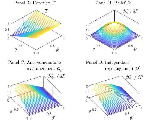
Case B: satisfies Assumption 1B. In this case, Theorem 1 does not follow from Proposition 1. This is because even if is independent (or IID), the anti-comonotone rearrangement in Proposition 1 is not necessarily independent (or IID). However, Proposition 2 shows that given an independent (or IID) belief, we can construct a rearrangement satisfying statements similar to Proposition 1 while preserving the independence (or IID) property.
Proposition 2.
Let be increasing in each argument and .
(i) If and are independent, there exists an independent and decreasing rearrangement of . Furthermore, if and are IID, then is IID.
(ii) Moreover, the expectation of is lower under than under :
Proof.
See Appendix A.2. ∎
Panel D of Figure 4 illustrates . Unlike the anti-comonotone rearrangement in Proposition 1, the upper contour sets of do not coincide with the lower contour sets of . However, the upper contour sets of have greater intersections with the lower contour sets of than the upper contour sets of have. This means that assigns greater probabilities to low values of and smaller probabilities to high values of than does. Hence, the expectation of is lower under than under .
4 Comparison between commonly studied auctions
In this section, assuming that the reference belief is IID, we apply Theorem 2 to compare the worst-case revenues of four commonly studied auctions: the first-price auction (I), second-price auction (II), all-pay auction (A) and (static) war of attrition (W). For simplicity, we assume no reserve price; however, the extension to reserve prices is straightforward.
Since the bidders are assumed to be ambiguity neutral, the equilibrium bidding strategies and transfer functions for the four auctions are given as follows (see, e.g., Milgrom, 2004):
where denotes the marginal cumulative distribution of and denotes its marginal probability density.
Theorem 3, the main result of this section, establishes the worst-case revenue rankings between the four auctions (Figure 5).
Theorem 3.
Suppose satisfies Assumption 1A or 1B. If is IID and the bidders are ambiguity neutral, the following statements hold:
(i) .
(ii) .
(iii) .
(iv) Suppose that
| increases in . | (11) |
Then, .
Proof.
See Appendix D. ∎
Condition (11) is a weak version of the usual assumption that the hazard rate is increasing. This condition guarantees that the equilibrium bidding strategies of the second-price auction and war of attrition, and , intersect exactly once (except at the origin).888Condition (11) can be weakened because Theorem 3 (iv) holds whenever and intersect exactly once (except at the origin). For example, satisfies condition (11), where .
Notably, the worst-case revenue rankings in Theorem 3 are opposite to the expected revenue rankings in the affiliated values setup (Milgrom and Weber, 1982; Krishna and Morgan, 1997). Section 5 discusses the relationship between the two in detail. Also, in the special case of the bounded likelihood ratio model (Example 2 (b-IID)), Lo (1998) shows that the first-price auction outperforms the second-price auction. Theorem 3 (i) generalizes this result.999Lo (1998) also analyzes the case where both the seller and bidders have MMEU preferences, with the sets of priors given by the bounded likelihood ratio model. Likewise, this result is a special case of Corollary 1 (i) in Section 6.1.
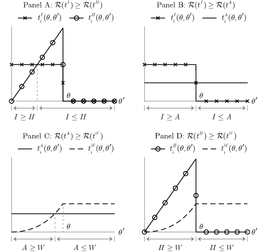
We now outline the proof of Theorem 3. By Theorem 2, to prove Theorem 3, it is sufficient to verify that the pairs satisfy both WSCC and RRC. Figure 6 illustrates that these pairs satisfy WSCC. Also, by the Revenue Equivalence Principle (Myerson, 1981), the four auctions yield the same interim expected revenues under ; hence, RRC holds as an equality. This establishes Theorem 3.
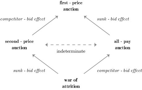
Analogously to Krishna and Morgan (1997), we identify two independent effects driving Theorem 3. To explain this, recall from Theorem 2 that a negative (or positive) association between a bidder’s payment and her competitor’s type increases (or decreases) worst-case revenue. First, auctions in which a bidder pays the competitor’s bid underperform auctions in which a bidder pays her own bid; we name this the competitor-bid effect (Figure 5, arrows with upper-right directions). When a bidder pays the competitor’s bid instead of her bid, a positive association between her payment and the competitor’s type arises. According to Theorem 2, this positive association decreases worst-case revenue. The competitor-bid effect explains why the second-price auction underperforms the first-price auction, and the war of attrition underperforms the all-pay auction.
Second, auctions in which bids are sunk underperform auctions in which payments are contingent on winning; we name this the sunk-bid effect (Figure 5, arrows with upper-left directions). The logic is similar as in the previous paragraph: the fact that a bidder pays even when she loses—in which case the competitor’s type is high—creates a positive association between her payment and the competitor’s type. The sunk-bid effect explains why the all-pay auction underperforms the first-price auction, and the second-price auction underperforms the war of attrition.
The ranking between the second-price and all-pay auctions is indeterminate, as shown in Figure 7. This is because whereas the competitor-bid effect makes the second-price auction inferior to the all-pay auction, the sunk-bid effect offsets this effect.
5 Relation to the Linkage Principle
As mentioned in Section 4, the worst-case revenue rankings between the four auctions in Theorem 3 are opposite to the expected revenue rankings in the affiliated values setup (Milgrom and Weber, 1982; Krishna and Morgan, 1997). By investigating the relationship between Theorem 2 and the Linkage Principle, this section explains why the two results are opposite.
We first introduce some notation and terminology. Let be the probability density of . Recall that is symmetric if , and is affiliated if for all ,
In this section, we focus on symmetric auctions in which the highest bidder wins. Consider an auction with a symmetric and increasing equilibrium. Let and be the unconditional expected payment and the expected payment conditional on winning when bidder with type reports :
Also, denotes the partial derivative with respect to the second argument.
Next, recall the Linkage Principle:
Theorem 4 (Linkage Principle; Krishna, 2002, Ch. 7).
Assume is symmetric and affiliated. Let and be auctions with symmetric and increasing equilibria satisfying . Suppose that either of the following two conditions holds:
(i) Linkage Condition-Version 1 (LC1). For all and ,
(ii) Linkage Condition-Version 2 (LC2). The loser pays nothing in both and . In addition, for all and ,
Then,
According to Theorem 2, when is IID, WSCC implies that yields a higher worst-case revenue than (recall that RRC automatically holds by the Revenue Equivalence Principle). On the contrary, according to the Linkage Principle, when is symmetric and affiliated, LCs imply that yields a higher expected revenue than . Proposition 1 below shows that between the four auctions studied in Section 4, WSCC holds if and only if either of the two LCs holds. Thus, Theorem 2 and the Linkage Principle work in the opposite directions. This explains why the worst-case revenue rankings in Theorem 3 are opposite to the expected revenue rankings with affiliated values.
Proposition 1.
For , the following conditions are equivalent:
(i) Under any IID , satisfies WSCC.
(ii) Under any symmetric and affiliated such that and have symmetric and increasing equilibria,101010The first-price and second-price auctions have equilibria whenever is symmetric and affiliated. Krishna and Morgan (1997) provide sufficient conditions on for equilibrium existence in the all-pay auction and war of attrition, omitted in our paper due to space limitation. satisfies either LC1 or LC2.
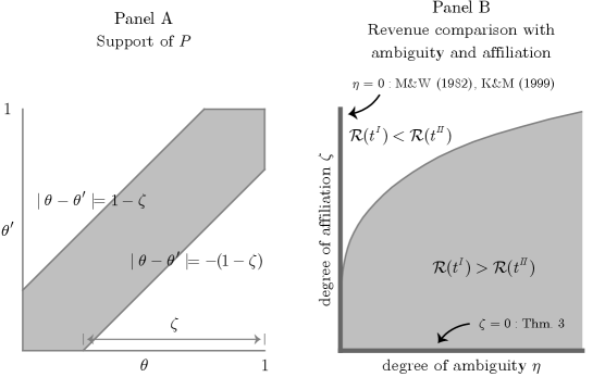
Let be the relative entropy neighborhood (Example 1 (a)): . Also, let be uniform over , illustrated in Panel A. If , types are independent; if , types are perfectly affiliated. The parameters and represent the degrees of ambiguity and affiliation, respectively.
Panel B compares the worst-case revenues of the first-price and second-price auctions for each . In the shaded region where ambiguity dominates affiliation, the ranking is the same as in Theorem 3. By contrast, in the white region where affiliation dominates ambiguity, the ranking is the same as in Milgrom and Weber (1982) and Krishna and Morgan (1997).
Intuitively, WSCC means that a bidder’s payment is more negatively associated with her competitor’s type in than in . On the other hand, the standard interpretation of LCs is that a bidder’s payment is more negatively associated with her own type in than in . However, a negative association between a bidder’s payment and her competitor’s type creates a negative association between her payment and her own type in the affiliated value setup. As a result, WSCC and LCs hold simultaneously.
A direct implication of Proposition 1 is that in the presence of both ambiguity and affiliation, the revenue rankings between the four auctions in Section 4 are indeterminate. When the effect of ambiguity dominates the effect of affiliation, the ranking is the same as in Theorem 3; in the opposite case, the ranking is the same as in Milgrom and Weber (1982) and Krishna and Morgan (1997). Figure 8 illustrates this fact by comparing the first-price and second-price auctions. Comparisons between other pairs of auctions yield similar results.
6 Extensions
This section presents two extensions: ambiguity averse bidders (Section 6.1) and ambiguity seeking seller (Section 6.2).
6.1 Ambiguity averse bidders
Existing studies on auctions with ambiguity mostly focus on the implications of the bidders’ ambiguity aversion (Table 1; see also Section 7.1). This section partially extends our results to the setup in which both the seller and bidders exhibit ambiguity aversion. Specifically, assuming that the reference belief is IID, we show that the worst-case revenue comparison results between the four auctions remain unchanged, except for the case between the second-price auction and war of attrition.
|
|
|
|||||||||||
|
|
|
Section 6.2 | ||||||||||
|
|
|
- |
We represent a bidder’s belief about the competitor’s type by its cumulative distribution function . Also, denote a bidder’s reference belief by . Each bidder holds a set of priors (assumed to be weakly compact) that satisfies the following assumption:
Assumption 3.
(i) .
(ii) is rearrangement invariant with respect to .
Consider a symmetric sealed-bid auction in which a bidder wins the object with probability and pays when she bids and the competitor bids . A bidding strategy is a symmetric equilibrium if
Then, the transfer function is given by .
Existing studies provide closed-form formulas for the equilibria of the first-price, second-price and all-pay auctions (Lo, 1998; Baik and Hwang, 2021). Regarding the war of attrition, although an implicit characterization of equilibrium is available, a sufficient condition for the existence of equilibrium is unknown. As the investigation of this problem is beyond the scope of this paper, we simply assume the existence of equilibrium when necessary.
Now, we compare the worst-case revenues of the four auctions in Section 4. Because Theorem 2 imposes no restrictions on the bidders’ preferences, it is applicable to the current setup. Therefore, to show that the seller prefers auction to auction , it suffices to verify WSCC and RRC. Arguing as in Section 4, it is straightforward to prove that the pairs satisfy WSCC (provided that the war of attrition has an equilibrium). In addition, Proposition 1, proven by Baik and Hwang (2021), shows that these pairs of auctions satisfy RRC:111111Baik and Hwang’s (2021) assumption on the bidders’ sets of priors differs from ours. However, their proofs are valid as long as the following property holds: for any bounded measurable and a -algebra , Cerreia-Vioglio et al. (2012, Thm. 2) show that Assumption 3 implies this property.
Proposition 1 (Baik and Hwang, 2021).
Suppose is IID and satisfies Assumption 3. Then, for all and ,
(i) .
(ii) .
(iii) If the war of attrition has an equilibrium, .
As a result, we obtain Corollary 1, which states that Theorem 3 (i)-(iii) remain valid when the bidders are ambiguity averse.
Corollary 1.
(i) .
(ii) .
(iii) If the war of attrition has an equilibrium, .
The primary difficulty with extending Theorem 3 (iv), which compares the second-price auction and war of attrition, lies in the complexity of the equilibrium characterization of the war of attrition.
Remark 1.
Auster and Kellner (2022) analyze the Dutch auction with ambiguity averse bidders. They find that due to dynamic inconsistency, the strategic equivalence between the Dutch and first-price auctions breaks down, and the equilibrium bidding strategy of the Dutch auction is higher than that of the first-price auction. This result, combined with Corollary 1, implies that when both the seller and bidders exhibit ambiguity aversion, the Dutch auction outperforms the four static auctions studied in this section.
6.2 Ambiguity seeking seller
Experimental evidence shows that there is substantial heterogeneity in individuals’ attitudes toward ambiguity, and some individuals are ambiguity seeking (Ahn et al., 2014; Chandrasekher et al., 2022). This section studies the setup in which the seller displays an ambiguity seeking preference. That is, she evaluates an auction by the best-case revenue , defined as
Proposition 2 states that if auctions and satisfy the opposite condition to WSCC—named the Negative Weak Single-Crossing Condition (NWSCC)—and RRC, then the ambiguity seeking seller prefers to . The name NWSCC is derived from the fact that it requires the negatives of transfer functions to satisfy WSCC: i.e., and satisfy NWSCC if and only if and satisfy WSCC.
Proposition 2.
Suppose satisfies Assumption 1A or 1B. Let and be auctions satisfying Assumption 2. Consider the following condition:
Negative Weak Single-Crossing Condition (NWSCC). For all and , there exists a threshold such that
If satisfies NWSCC and RRC, then .
As an immediate consequence, revenue comparisons between the four auctions yield opposite results to the ambiguity aversion case: when is IID, (i) the war of attrition outperforms the second-price and all-pay auctions, and (ii) the second-price and all-pay auctions outperform the first-price auction. In other words, the best-case revenue rankings between the four auctions reproduce the expected revenue rankings in the affiliated values setup (Milgrom and Weber, 1982; Krishna and Morgan, 1997).
Because the two rankings are identical, unlike the ambiguity aversion case in Section 5, the best-case revenue rankings extend to the case in which is symmetric and affiliated. Specifically, using the equilibrium bidding strategies in the affiliated values setup (Milgrom and Weber, 1982, Thm. 6 and 14; Krishna and Morgan, 1997, Thm. 1-2), it can be shown that the pairs satisfy NWSCC. In addition, the proofs of the expected revenue rankings in the affiliated values setup (Milgrom and Weber, 1982, Thm. 15; Krishna and Morgan, 1997, Thm. 3-5) show that the same rankings also hold for interim expected revenues; this implies that the above pairs of auctions satisfy RRC. Thus, by Proposition 2, the best-case revenue rankings remain valid when is symmetric and affiliated.
7 Discussion
7.1 Related literature
Auctions with ambiguity. This paper is most closely related to the literature on auctions with ambiguity. While existing works mainly focus on the bidders’ ambiguity aversion (Bose and Daripa, 2009; Bodoh-Creed, 2012; Ghosh and Liu, 2021; Auster and Kellner, 2022), Bose et al. (2006, Sec. 6) show that when the seller is ambiguity averse and bidders are ambiguity neutral, the optimal mechanism is a seller-full-insurance auction where the total transfer is constant in the type profile. Bose et al. (2006, Sec. 3) also show that when the seller and bidders are both ambiguity averse but the seller is less averse than the bidders, the optimal mechanism is a bidder-full-insurance auction where a bidder’s payoff is constant with respect to the competitor’s type. However, because these two mechanisms depend on the bidders’ beliefs, they are difficult to implement in practice and hence rarely used in reality (Wilson, 1987). We complement their results by comparing easily implementable auctions. Also, under a specific parametrization of the set of priors (Example 2 (b-IID)), Lo (1998) compares the first-price and second-price auctions. As mentioned in Section 4, our paper includes this result as a special case.
Robust auction design. This paper is also related to the robust auction design literature (Bergemann et al., 2017, 2019; Brooks and Du, 2021; Che, 2022; Suzdaltsev, 2022; He and Li, 2022). Our assumption on the seller’s ambiguity set differs from this literature. Existing works consider the minimum expected revenues over (i) all information structures between valuations and signals with a given valuation distribution (Bergemann et al., 2017, 2019; Brooks and Du, 2021), (ii) all valuation distributions satisfying certain moment conditions (Che, 2022; Suzdaltsev, 2022), or (iii) all correlation structures between valuations with a given marginal valuation distribution (He and Li, 2022). By contrast, our set of priors consists of beliefs that are close to the reference belief, the so-called discrepancy-based model (Rahimian and Mehrotra, 2019). Despite its popularity in other strands of the literature—e.g., the macroeconomics literature on model misspecification (Hansen and Sargent, 2001, 2008) and the operations research literature on robust optimization (Ben-Tal et al., 2013)—the discrepancy-based model has been less frequently used in the literature on auctions where the seller has limited information about the valuation distribution. Our study shows that interesting revenue comparison results—those opposite to the Linkage Principle results—arise for discrepancy-based sets of priors.
7.2 Conclusion
This paper studies the revenue comparison problem of auctions when the seller has an MMEU preference. Assuming rearrangement invariance of the set of priors, we develop a methodology to compare the worst-case revenues. As an application, we compare the worst-case revenues of four commonly studied auctions: the first-price, second-price, all-pay auctions and war of attrition. Our methodology yields results opposite to those of the Linkage Principle.
Although this paper focuses on the four auctions, our methodology applies to a broader range of mechanisms. For instance, Siegel (2010) studies a mechanism in which the winner pays her bid and the loser pays a fixed fraction of her bid, called a simple contest. This mechanism can be regarded as a convex combination of the first-price and all-pay auctions. Applying Theorem 2, it can be shown that the worst-case revenue of a simple contest decreases in the fraction of the bid paid by the loser. In other words, the closer a simple contest is to the first-price auction (equivalently, the farther it is from the all-pay auction), the higher the worst-case revenue it generates. Similar conclusions hold for the convex combinations of the other auction pairs studied in Section 4.
Following most of the literature on auctions with ambiguity, our paper assumes that the seller has an MMEU preference. However, our results carry over to the setup in which the seller has an uncertainty averse preference, a generalization of the MMEU preference axiomatized by Cerreia-Vioglio et al. (2011). Under rearrangement invariance assumptions analogous to Assumptions 1A-1B (see Cerreia-Vioglio et al., 2011, Sec. 4.1), it is straightforward to extend Theorems 1-3. In particular, uncertainty averse preferences include divergence preferences as a special case (Maccheroni et al., 2006), represented by
where is defined in Example 1 (a) and represents the degree of ambiguity. This preference, along with the MMEU preference, is one of the most popular models in the robustness literature (Hansen and Sargent, 2001, 2008).
Appendix
A Rearrangement inequalities
Throughout this section, we repeatedly use the following well-known fact in probability theory. Suppose that is an atomless probability measure on , and is the cumulative distribution of :
Then,
| (12) |
In other words, if is distributed according to , then is uniformly distributed over .
Also, for an increasing function such that and , define its right-continuous inverse as follows (see, e.g., Föllmer and Schied, 2016, Sec. A.3):
A.1 Proof of Proposition 1
(i) Let be the cumulative distributions of and :
| for all , | ||||
| (13) |
Applying equation (12) with and (note that is atomless by condition (8)), we have
| (14) |
That is, if is distributed according to , then is uniformly distributed over .
A.2 Proof of Proposition 2
Proof of Proposition 2 (i).
Let . It is evident from Appendix A.1 that Proposition 1 (i) holds even if we replace with . Applying this result with defined as , there exists a rearrangement of satisfying condition (9) (more precisely, its one-dimensional version). Since is increasing, condition (9) implies that is decreasing. Now, let . Then, is an independent and decreasing rearrangement of . Also, by construction, if and are IID, then is IID.
∎
To prove Proposition 2 (ii), as in the proofs of classical rearrangement inequalities (Lieb and Loss, 2001, Ch. 3), we first consider the simplest case where , and are indicator functions:
| (16) |
Lemma 1.
Assume is independent. Suppose that is an event such that
| (17) |
Let be events with . Also, let be intervals with left endpoint satisfying and . Then,
| (18) |
Panel A of Figure 9 illustrates Lemma 1. As we show later, once Lemma 1 is established, Proposition 2 (ii) follows by a standard argument.
Proof of Lemma 1.
We proceed in three steps.
Step 1. Without loss of generality, we can assume is uniform over .
Let be the uniform probability measure on . Also, for , denote the cumulative distribution of as . Define
By equation (12), if is distributed according to , then is distributed according to . Using this fact, it is straightforward to verify the following:
(i) satisfies condition (17).
(ii) is an interval with left endpoint satisfying .
(iii) Inequality (18) is equivalent to
Hence, by replacing , , and with , , and , respectively, we can always assume .
Panel B of Figure 9 illustrates Step 2. First, since is assumed to be uniform over (Step 1), by definition (16),
| (21) |
Next, by definitions (16) and (19), is the cumulative distribution of . Hence, by equation (12),
| (22) |
Then, equations (21)-(22) imply
If two measures coincide for sets of the form , they must be equal. Hence,
By independence, equation (20) holds.
Step 3. The desired inequality (18) holds.
First, by definition (16),
| (23) |
Next, Step 2 shows that if is distributed according to , then is distributed according to .131313More precisely, is the image measure of induced by . By the change of variables formula for Lebesgue integration (Shiryaev, 1996, Thm. 7 of Sec. II.6),
| (24) |
Now, by definition, . By property (17), whenever , we have . It follows that . Hence
| (25) |
Finally, by the same argument as in equation (A.2),
| (26) |
∎
Proof of Proposition 2 (ii).
By the Layer Cake Representation (see, e.g., Lieb and Loss, 2001, Sec. 1.13 and Sec. 3.4) and Fubini’s theorem,
By the same reason,
Therefore, to prove the desired inequality , it suffices to prove the following: for all ,
| (27) |
To prove inequality (27), fix . Let
If , inequality (27) holds because both sides are zero. Next, suppose . We show that the hypothesis of Lemma 1 holds. First, because is increasing, satisfies condition (17). Also, recall from the proof of Proposition 2 (i) that is a decreasing rearrangement of . This implies that , and is an interval with left endpoint zero. Thus, by Lemma 1, inequality (27) holds.
∎
B Proof of Theorem 2
Let be given. As argued in Section 3, to prove Theorem 2, it suffices to prove the following: for all and such that ,
| (28) |
Note that condition ensures that is well-defined.
Fix and . By WSCC, there exists such that
Let be the Radon-Nikodym derivative of with respect to . Since decreases in each argument, decreases in . Hence,
where . By the same reason,
where . Thus,
where the last inequality holds by RRC. This establishes inequality (28).
C Weak Single-Crossing Condition
In this section, we prove the equivalence between WSCC and condition (7). To show this, it is sufficient to show Proposition 1 below:
Proposition 1.
Let . The following conditions are equivalent:
(i) There exists such that for all ,
(ii) For all ,
Proof.
Without loss of generality, assume .
(i) (ii). Suppose that and . Condition (i) implies that . Since , it follows by condition (i) that .
(ii) (i). We divide into two cases.
Case 1: If . In this case, define . Then, for , we have by definition. Next, suppose . By the property of the infimum, there exists such that . Condition (ii) implies that .
Case 2: If . In this case, for all . Hence, if we let , then condition (i) holds.
∎
D Proof of Theorem 3
By Theorem 2, to prove Theorem 3, it suffices to show that the pairs satisfy WSCC and RRC. By the Revenue Equivalence Principle (Myerson, 1981), RRC holds. It remains to verify WSCC.
(i) . Given and , let . Then, since ,
(ii) . Given and , let . It is straightforward to show that . Hence,
(iii) . Note first that
| (29) |
where the third inequality holds because for .
Now, let and be given. By inequality (D) and continuity, there exists such that . Then,
(iv) . We proceed in three steps.
Step 1. .
Suppose on the contrary that , where the limit exists by condition (11). Condition (11) implies further that for all . Hence, for all with ,
| (30) |
However, if we take the limit , the left-hand side converges to , whereas the right-hand side diverges to infinity. Hence, inequality (30) cannot hold for sufficiently small values of , a contradiction.
Step 2. There exist such that
| (31) |
By definition, . Also, by Step 1, . It follows that for all sufficiently close to , we have . Furthermore, Krishna and Morgan (1997, Prop. 1) show that . Hence, for all sufficiently close to , we have . Hence, there exists an intersection satisfying . Because condition (11) implies that is convex, property (31) holds.
Step 3. satisfies WSCC. Given and , we divide into two cases.
Step 3-Case 1: If . Let . Then,
| for , | |||
| for , |
Step 3-Case 2: If . Let . Then,
| for , | |||
| for , | |||
| for , | |||
| for , |
E Proof of Proposition 1
We claim that satisfy both conditions (i) and (ii), and the others satisfy neither.
Condition (i). In the proof of Theorem 3, we have already shown that satisfy WSCC. Also, a similar argument shows that satisfies WSCC. It straightforward to check that the remaining pairs of auctions do not satisfy WSCC.
Condition (ii). First, Krishna (2002, Sec. 7.1-7.2) shows that satisfies LC2 and satisfies LC1.
Also, to see that satisfies LC1, note that since is constant in , we have . However, since increases in , affiliation implies that . Hence, satisfies LC1.
Next, we show that satisfies LC1. When bidder has type , denote the cumulative distribution and the probability density of the competitor’s type as and . Also, let be the hazard rate:
It is well-known that decreases in (Krishna and Morgan, 1997, Fact 3).
Krishna and Morgan (1997, proof of Thm. 3) show that
Hence, to prove that satisfies LC1, it suffices to show that
| (32) |
To prove inequality (32), note that because decreases in ,
| (33) |
Also, by the same reason, for ,
Taking the limit yields
| (34) |
Finally, satisfies LC1 because satisfy LC1. It is easy to verify that the remaining pairs satisfy neither LC1 nor LC2.
References
- Ahn et al. (2014) Ahn, D., Choi, S., Gale, D., Kariv, S., 2014. Estimating ambiguity aversion in a portfolio choice experiment. Quantitative Economics 5, 195–223.
- Ali and Silvey (1966) Ali, S.M., Silvey, S.D., 1966. A general class of coefficients of divergence of one distribution from another. Journal of the Royal Statistical Society 28, 131–142.
- Auster and Kellner (2022) Auster, S., Kellner, C., 2022. Robust bidding and revenue in descending price auctions. Journal of Economic Theory 199, 105072.
- Baik and Hwang (2021) Baik, S., Hwang, S.H., 2021. Auction design with ambiguity: Optimality of the first-price and all-pay auctions. ArXiv:2110.08563.
- Ben-Tal et al. (2013) Ben-Tal, A., den Hertog, D., Waegenaere, A.D., Melenberg, B., Rennen, G., 2013. Robust solutions of optimization problems affected by uncertain probabilities. Management Science 59, 341–357.
- Bergemann et al. (2017) Bergemann, D., Brooks, B., Morris, S., 2017. First-price auctions with general information structures: Implications for bidding and revenue. Econometrica 85, 107–143.
- Bergemann et al. (2019) Bergemann, D., Brooks, B., Morris, S., 2019. Revenue guarantee equivalence. American Economic Review 109, 1911–1929.
- Bodoh-Creed (2012) Bodoh-Creed, A.L., 2012. Ambiguous beliefs and mechanism design. Games and Economic Behavior 75, 518–537.
- Bose and Daripa (2009) Bose, S., Daripa, A., 2009. A dynamic mechanism and surplus extraction under ambiguity. Journal of Economic Theory 144, 2084–2114.
- Bose et al. (2006) Bose, S., Ozdenoren, E., Andreas, P., 2006. Optimal auctions with ambiguity. Theoretical Economics 1, 411–438.
- Brooks and Du (2021) Brooks, B., Du, S., 2021. Optimal auction design with common values: An informationally robust approach. Econometrica 89, 1313–1360.
- Cerreia-Vioglio et al. (2011) Cerreia-Vioglio, S., Maccheroni, F., Marinacci, M., Montrucchio, L., 2011. Uncertainty averse preferences. Journal of Economic Theory 146, 1275–1330.
- Cerreia-Vioglio et al. (2012) Cerreia-Vioglio, S., Maccheroni, F., Marinacci, M., Montrucchio, L., 2012. Probabilistic sophistication, second order stochastic dominance and uncertainty aversion. Journal of Mathematical Economics 48, 271–283.
- Chandrasekher et al. (2022) Chandrasekher, M., Frick, M., Iijima, R., Yaouanq, Y.L., 2022. Dual-self representations of ambiguity preferences. Econometrica 90, 1029–1061.
- Che (2022) Che, E., 2022. Robustly optimal auction design under mean constraints. Proceedings of the 23rd ACM Conference on Economics and Computation , 153–181.
- Che and Gale (1998) Che, Y.K., Gale, I., 1998. Standard auctions with financially constrained bidders. The Review of Economic Studies 65, 1–21.
- Ellsberg (1961) Ellsberg, D., 1961. Risk, ambiguity, and the Savage axioms. Quarterly Journal of Economics 75, 643–669.
- Föllmer and Schied (2016) Föllmer, H., Schied, A., 2016. Stochastic Finance: An Introduction in Discrete Time. Fourth ed., De Gruyter, Berlin.
- Ghirardato and Marinacci (2002) Ghirardato, P., Marinacci, M., 2002. Ambiguity made precise: A comparative foundation. Journal of Economic Theory 102, 251–289.
- Ghosh and Liu (2021) Ghosh, G., Liu, H., 2021. Sequential auctions with ambiguity. Journal of Economic Theory 197, 105324.
- Ghossoub (2015) Ghossoub, M., 2015. Equimeasurable rearrangements with capacities. Mathematics of Operations Research 40, 429–445.
- Gilboa and Schmeidler (1989) Gilboa, I., Schmeidler, D., 1989. Maxmin expected utility with non-unique prior. Journal of Mathematical Economics 18, 141–153.
- Hansen and Sargent (2001) Hansen, L.P., Sargent, T., 2001. Robust control and model uncertainty. American Economic Review 91, 60–66.
- Hansen and Sargent (2008) Hansen, L.P., Sargent, T., 2008. Robustness. Princeton University Press.
- Hardy et al. (1959) Hardy, G.H., Littlewood, J.E., Pólya, G., 1959. Inequalities. Cambridge University Press.
- He and Li (2022) He, W., Li, J., 2022. Correlation-robust auction design. Journal of Economic Theory 200, 105403.
- Krishna (2002) Krishna, V., 2002. Auction theory. Academic Press.
- Krishna and Morgan (1997) Krishna, V., Morgan, J., 1997. An analysis of the war of attrition and the all-pay auction. Journal of Economic Theory 72, 343–362.
- Kullback and Leibler (1951) Kullback, S., Leibler, R.A., 1951. On information and sufficiency. The Annals of Mathematical Statistics 22, 79–86.
- Lieb and Loss (2001) Lieb, E., Loss, M., 2001. Analysis. volume 14 of Graduate Studies in Mathematics. Second ed., American Mathematical Society, Providence, RI.
- Lo (1998) Lo, K.C., 1998. Sealed bid auctions with uncertainty averse bidders. Economic Theory 12, 1–20.
- Luxemburg (1967) Luxemburg, W.A.J., 1967. Rearrangement-invariant Banach function spaces. Queens Papers in Pure and Applied Mathematics 10, 83–144.
- Maccheroni et al. (2006) Maccheroni, F., Marinacci, M., Rustichini, A., 2006. Ambiguity aversion, robustness, and the variational representation of preferences. Econometrica 74, 1447–1498.
- Machina and Schmeidler (1992) Machina, M.J., Schmeidler, D., 1992. A more robust definition of subjective probability. Econometrica 60, 745–780.
- Maskin and Riley (1984) Maskin, E., Riley, J., 1984. Optimal auctions with risk averse buyers. Econometrica 52, 1473–1518.
- Maskin and Riley (2000) Maskin, E., Riley, J., 2000. Asymmetric auctions. The Review of Economic Studies 67, 413–438.
- Milgrom (2004) Milgrom, P., 2004. Putting Auction Theory to Work. Cambridge University Press, Cambridge, UK.
- Milgrom and Weber (1982) Milgrom, P., Weber, R., 1982. A theory of auctions and competitive bidding. Econometrica 50, 1089–1122.
- Myerson (1981) Myerson, R.B., 1981. Optimal auction design. Mathematics of Operations Research 6, 58–73.
- Rahimian and Mehrotra (2019) Rahimian, H., Mehrotra, S., 2019. Distributionally robust optimization: A review. ArXiv:1908.05659.
- Safra and Segal (1998) Safra, Z., Segal, U., 1998. Constant risk aversion. Journal of Economic Theory 83, 19–42.
- Shaked and Shanthikumar (1994) Shaked, M., Shanthikumar, J., 1994. Stochastic orders and their applications. Academic Press, San Diego, CA.
- Shiryaev (1996) Shiryaev, A.N., 1996. Probability. Second ed., Springer-Verlag, New York.
- Siegel (2010) Siegel, R., 2010. Asymmetric contests with conditional investments. American Economic Review 100, 2230–2260.
- Suzdaltsev (2022) Suzdaltsev, A., 2022. Distributionally robust pricing in independent private value auctions. Journal of Economic Theory (In Press), 105555.
- Waehrer et al. (1998) Waehrer, K., Harstad, R.M., Rothkopf, M.H., 1998. Auction form preferences of risk-averse bid takers. RAND Journal of Economics 29, 179–192.
- Wilson (1987) Wilson, R., 1987. Game-theoretic analyses of trading processes, in: Bewley, T. (Ed.), Advances in Economic Theory: Fifth World Congress. Cambridge University Press, Cambridge. chapter 2, pp. 33–70.
- Yaari (1987) Yaari, M.E., 1987. The dual theory of choice under risk. Econometrica 55, 95–115.