Review on Determining the Number of Communities in Network Data

Network-structured data and network analysis are garnering increasing attention across various fields. Research in this area often focuses on understanding the structure of network data, with significant implications for social sciences, biology, and statistics. The practical applications of this research profoundly impact our daily lives in multiple ways. For example, search engines utilize discoveries and tools from this field to analyze the relationships among various keywords. See Kolaczyk and Csárdi, (2014), Hevey, (2018), Sun and Han, (2013), and Berkowitz, (2013) for further reading.

Community detection is of major interest of network analysis. Given an $n$-node (undirected) graph $(\mathcal{N},E)$, where $\mathcal{N}=\{1,2,...n\}$ is the set of nodes and $E$ is the set of edges. We assume that $\mathcal{N}$ could be partitioned into $K$ disjoint subsets or ”communities”. The community structure is represented by a vector $g=(g_{1},...,g_{n})$ with $g_{i}\in\{1,...,K\}$ being the community that node $i$ belongs to. Nodes tend to have more common characteristics in the same communities. Various algorithms have been proposed to partition these nodes. However, most of them must fixed $K$ as a priori. How to determine $K$ priori is still an open problem.

Bickel and Sarkar, (2016) proposed a testing statistics based on the limiting distribution of the principal eigenvalue of the suitably centred and scaled adjacency matrix. However they only have theoretical results for testing null hypothesis of $H_{0}:K=1$. For testing $H_{0}:K=j$ when $j>1$, they need to iteratively split the network into small sub-networks. It seems that their testing statistics does not work well on the later one. Compared to stochastic block model (SBM), degree corrected block model (DCBM) proposed by Karrer and Newman (2011) is more flexible. Jin, (2015) proposed a so called spectral clustering on ratios-of-eigenvectors (SCORE) method to detect communities for DCBM. The idea is by clustering on entry-wise ratio of eigenvectors of the adjacency matrix. Taking the ratio can eliminate the effect of degree heterogeneity. Further Ji et al., (2016) apply SCORE to a practical problem on detecting potential communities in coauthorship and citation networks for statisticians. However, there are few works on the hypothesis testing of $K$ targetedly for DCBM. Instead of performing hypothesis testing, Chen and Lei, (2018) proposed a specially designed cross-validation method to figure out $K$. In the following, we are going to give a brief review and duplicate the numerical results of some of the aforementioned papers.

In an SBM with $n$ nodes and $K$ communities, Let $A$ be the adjacency matrix. and $g=(g_{1},...,g_{n})$ with $g_{i}\in\{1,...,K\}$ being the community that node $i$ belongs to. Given the membership vector $g$, each edge $A_{ij}(i<j)$ is an independent Bernoulli variable satisfying

where $B$ is a $K\times K$ symmetric matrix representing the community-wise edge probabilities.

Bickel and Sarkar, (2016) proposed a statistics on testing problem with null hypothesis $H_{0}:K=1$ based on some properties of Erdős-Renýi graph. In their paper, they assume that the number of clusters $K$ and the edge probabilities are constant, whereas the number of nodes $n$ is growing to $\infty$. Thus the average degree is growing linearly with $n$. In addition Cragg and Donald, (1993), Cragg and Donald, (1997), Cui et al., 2024b , Cui et al., 2024a Du, (2025) and Cui et al., (2023) discussed about rank inference of a matrix, which can be a generalization work of Bickel and Sarkar, (2016).

Noticing that Erdős-Renýi graph can be viewed as a special case of SBM when there is only one community and one community-wise edge probability $p:=B_{11}$. We can estimate it within $O_{P}(1/n)$ error by computing the proportion of pairs of nodes that forms an edge, denoted by $\widehat{p}$.

Let $\widehat{P}:=n\widehat{p}\mathbf{e}\mathbf{e}^{\mathrm{T}}-\widehat{p}I$, which is an estimate for the mean of adjacency matrix. Bickel and Sarkar, (2016) proved the following theorem:

Example 1. Here we performed a simulation study to see the size performance of the testing statistics. We construct a Erdős-Renýi graph with $n=500$. $p$ ranges from 0.1 to 0.9, increasing with 0.1 in each step.

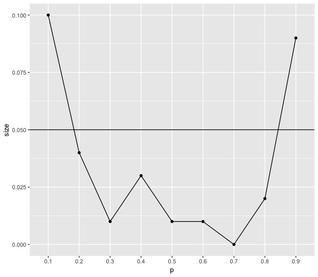
We can see from the simulation study that they cannot control the size. The author proposed a small sample correction on their testing statistics. That is due to the low convergence rate of the eigenvalues, whereas the largest eigenvalues of GOE matrices converge to the Tracy–Widom distribution quite quickly, those of adjacency matrices do not. Based on that, they proposed a small sample correction which suggests that computing the $p$-value by using the empirical distribution of $\lambda_{1}$ generated by using a parametric bootstrap step. The main idea is to compute the mean and the variance of the distributions from a few simulations, and then shift and scale the test statistic to match the first two moments of the limiting TW₁ law. Table 1 shows the whole algorithm for perfoming the hypothesis proposed in Bickel and Sarkar, (2016).

In this section we want to look at a spectral clustering method for and DCBM, the SCORE method proposed by Jin, (2015).

In a DCBM, given membership vector $g$ and community-wise connectivity matrix $B$, Let $\psi$ and $\Psi$ be the $n\times 1$ vector and the $n\times n$ diagonal matrix defined as follows:

The presence of an edge between nodes $i$ and $j$ is represented by a Bernoulli random variable $A_{ij}$ with

The main difference between DCBM and SBM is the appearance of the degree heterogeneity parameter $\psi_{i}>0$. $\psi_{i}$ represents the individual activeness of node $i$. The idea of that is that some individuals in one group could be more outgoing than others, therefore edge probabilities are different for different individuals.

While the traditional spectral clustering method of SBM is simply by performing existing clustering methods on the eigenvectors of adjacency matrix, detecting communities with the DCBM is not an easy problem, where the main challenge lies in the degree heterogeneity.

The main observation of SCORE is that the effect of degree heterogeneity is largely an- cillary, and can be effectively removed by taking entry-wise ratios between eigenvectors. Let’s firstly consider the simple case when there are only two groups. Specifically, let

and denote $\Omega=E(A)$ Theorem 1 is

The key observation is that if we let $r$ be the $n\times 1$ vector of the coordinate- wise ratios between $\eta_{1}$ and $\eta_{2}$. $r_{i}=\dfrac{\eta_{2i}/\left\|\eta_{2}\right\|}{\eta_{1i}/\left\|\eta_{1}\right\|},\quad 1\leq i\leq n$. Then $r$ is independent from the degree heterogeneity parameter $\psi$.

Similar phenomenon also exists when there are $K>2$ groups.

Based on that, the algorithm of clustering on DCBM is proposed as following:

• •

  Let $\widehat{\eta}_{1}$ , $\widehat{\eta}_{2}$ ,…, $\widehat{\eta}_{K}$ be $K$ unit-norm eigenvectors of $A$ associated with the largest K eigenvalues (in magnitude), respectively.

• •

  Let $\widehat{R}$ be the $n\times K-1$ vector of coordinate-wise ratios: $\widehat{R}(i,k)=\widehat{\eta}_{k+1,i}/\widehat{\eta}_{1,i},\quad 1\leq k\leq K-1,1\leq i\leq n$

• •

  Clustering the labels by applying the k-means method to the vector $\widehat{R}$, assuming there are $\leq K$ communities in total.

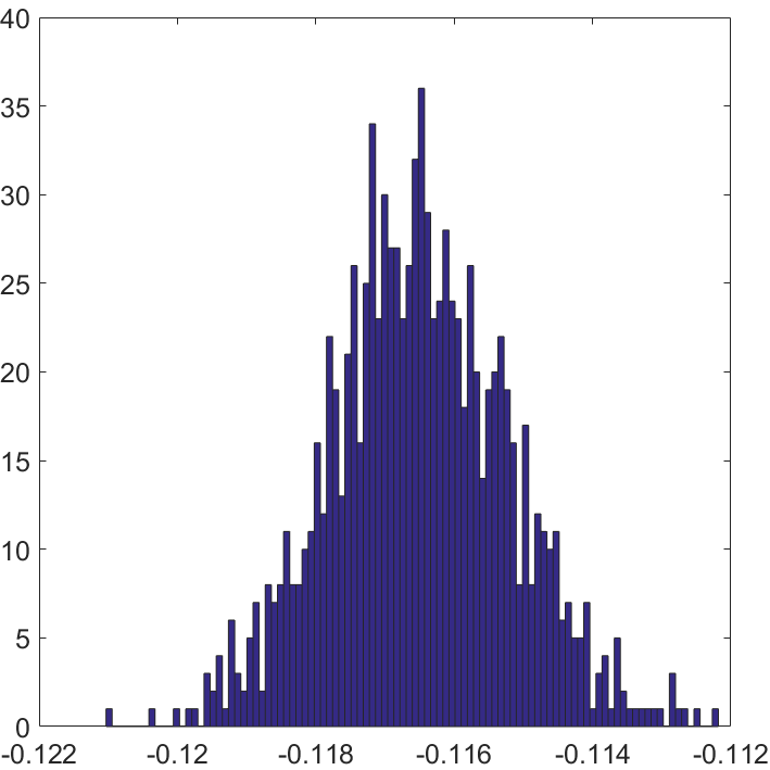
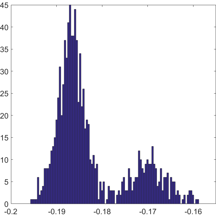
Example 2. Here I performed one simulation study to show the intuition of SCORE. We take $K=1$ and $K=2$ respectively to construct networks. For both we take $n=1000$ and generate $\bm{\psi}$ by $\text{log}(\psi_{i})\overset{i.i.d.}{\sim}N(0,0.2),1\leq i\leq n,$ then normalize $\psi$ by $\psi=0.9\cdot\psi/\psi_{\text{max}}.$ For $K=2$, 250 nodes are in different cluster with others. $B_{11}=B_{22}=1,B_{12}=0.5.$ The coordinate-wise plot is reported in Figure 2. Here when $K=1$, the $\widehat{R}$ is given by computing the coordinate ratio of $\eta_{1}$ and $\eta_{2}$. The patterns between $K=1$ and $K=2$ have significantly difference. If $K=1$, each coordinate of $\widehat{R}$ will gather around one constant as we showed before, while it will on two hierarchies rather than one when $K=2$.

Chen and Lei, (2018) proposed a network cross-validation (NCV) approach to determine the number of communities for both SBM and DCBM. It can automatically determine the number of communities based on a block-wise node-pair splitting technique. The main idea is that firstly, we randomly split the nodes into $V$ equal-sized subsets $\left\{\tilde{\mathcal{N}}_{v}:1\leq v\leq V\right\}$, and then split the adjacency matrix correspondingly into $V\times V$ equal sized blocks.

where $\tilde{A}^{(uv)}$ is the submatrix of $A$ with rows in $\tilde{N}_{u}$ and columns in $\tilde{\mathcal{N}}_{v}$. All the blocks are splitted into fitting sets and validation sets. We can estimate model parameters $\left(\widehat{g}^{(v)},\widehat{B}^{(v)}\right)$ using the rectangular submatrix as fitting set obtained by removing the rows of $A$ in subset $\tilde{N}_{v}$.

Then $\tilde{A}^{(vv)}$ is treated as validation sets and used to calculate the predictive loss. At last, $K$ is selected when the loss is minimized. In general, cross-validation methods are insensitive to the number of folds. The same intuition empirically holds true for the proposed NCV method. Here the author suggest to use $V=3$.

Take $V=2$ for example. We can rearrange adjacency matrix in a collapsed $2\times 2$ block form

Such a splitting puts node pairs in $A^{(11)}$ and $A^{(12)}$ as the fitting sample and those in $A^{(22)}$ as the validating sample. The advantages of that kind of splitting are from three aspects. Firstly, the fitting set carries full information about the network model parameters. We can consistently estimate the membership of all the nodes as well as the community-wise edge probability matrix, using only data in the fitting set. Secondly, given the community membership, the data in the fitting set and in the testing set are independent. Thirdly, it is different from cross validation methods for network data based on a node splitting technique. In the node splitting method, the nodes are usually split into a fitting set and a testing set. Therefore, one typically assumes that the node memberships are generated independently with prior probability $\pi=(\pi_{1},\pi_{2},\cdots,\pi_{K})$. However, it has several drawbacks. The main drawback is that calculating the full likelihood in terms of the prior probability in the presence of a missing membership vector $g$ is computationally demanding.

Algorithm details of their NCV method is shown as following:

• •

  Step 1: Block-wise node-pair splitting as shown in $(\ref{eq1})$

• •

  Step 2: Estimating model parameters from the fitting set.

  Take SBM for example.

  $$\begin{array}[]{l}{\text{ 1. Let }\widehat{U}\text{ be the }n\times d\text{ matrix consisting of the top }d\text{ right singular vectors of }A^{(1)}}\\ {\text{ 2. Output }\widehat{g}\text{ by applying the }k\text{ -means clustering with }\widetilde{K}\text{ clusters to the rows of\ }\widehat{U}.}\end{array}$$

  Once $\widehat{g}$ is obtained, let $\mathcal{N}_{j,k}$ be the nodes in $j$ with estimated membership $k$,and $n_{i,k}=\left|\mathcal{N}_{i,k}\right|(j=1,2,1\leq k\leq\tilde{K})$.Wecan estimate $B$ using a simple plug-in estimator:

  $$\widehat{B}_{k,k^{\prime}}=\left\{\begin{array}[]{ll}{\frac{\sum_{i\in\mathcal{N}_{1,k},j\in\mathcal{N}_{1,k^{\prime}}\cup N_{2,k^{\prime}}}A_{ij}}{n_{1,k}\left(n_{1,k^{+}}+n_{2,k^{\prime}}\right)},}&{k\neq k^{\prime}}\\ {\frac{\sum_{i,j\in\mathcal{N}_{1,k},i<j}A_{ij}+\sum_{i\in\mathcal{N}_{1,k},j\in\mathcal{N}_{2,k}A_{ij}}}{\left(n_{1,k}-1\right)n_{1,k}/2+n_{1,k}n_{2,k}},}&{k=k^{\prime}}\end{array}\right.$$

• •

  Step 3: Validation using the testing set. $\text{Consider the validated predictive loss }\widehat{L}(A,\widetilde{K})=\sum_{i,j\in\mathcal{N}_{2},i\neq j}\ell\left(A_{ij},\widehat{P}_{ij}\right)$, with $\text{ negative log-likelihood }\ell(x,p)=-x\log p-(1-x)\log(1-p)$ or squared error $\ell(x,p)=(x-p)^{2}$.

Algorithm of dealing with DCBM is similar. The only difference is that in step 2, we need to estimate the parameters $(g,B,\psi)$ under the framework of DCBM.

Example 3. I duplicate one of the simulation result in this paper. In the simulation study, the community-wise edge probability matrix $B=rB_{0}$, where the diagonal entries of $B_{0}$ are 3 and off-diagonal entries are 1. $n=1000,K=2$. The sparsity levels are chosen at $r\in\{0.01,0.02,0.05,0.1,0.2\}$. Size of the first community is set to be $n_{1}$ and size of second community is $n-n_{1}$. Figure 3 is the simulation result from 200 simulated data sets.

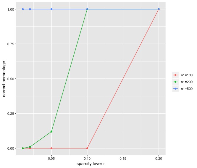
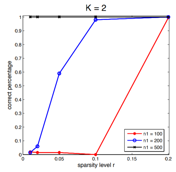
We can see that there is slight difference between my simulation result and that from the paper. The main difference is that when $n_{1}=200$ and sparsity level is $0.05$, I only observed a correct percentage of 0.12 but the author observed the The difference might come from the different choice of clustring method in Step 2 in the algorithm.

The author also gave theoretical properties for their NCV under SBM. They firstly introduce two notions of community recovery consistency. One is exactly consistent recovery. Given a sequence of SBMs with $K$ blocks parameterized by $\left(g^{(n)},B^{(n)}\right)$, we call a community recovery method $\widehat{g}$ exactly consistent if $P(\widehat{g}(A,K))=\left.g^{(n)}\right)\rightarrow 1$ where $A$ is a realization of SBM $\left(g^{(n)},B^{(n)}\right)$ and the equality is up to a possible label permutation. The other is called approximately consistent recovery. For a sequence of SBMs with $K$ blocks parameterized by $\left(g^{(n)},B^{(n)}\right)$ and a sequence $\eta_{n}=o(1)$, we say $\widehat{g}$ is approximately consistent with rate $\eta_{n}$ if,

where Ham($\widehat{g},g$) is the smallest Hamming distance between $\widehat{g}$ and $g$ among all possible label permutations.

NCV is proved to be approximately consistent with rate $(n\rho_{n})^{-1}$, with $\rho_{n}n/log(n)>C$ for some constant $C$. See Theorem 2 in Chen and Lei, (2018). Therefore it also has community recovery consistency property.

In this paper, we first examine the statistical approach proposed by Bickel and Sarkar, (2016) for hypothesis testing under the null hypothesis $H_{0}:K=1$. They derived the asymptotic null distribution of the largest eigenvalue of a suitably scaled and centered adjacency matrix. However, this method exhibits a slow convergence rate, necessitating bootstrap corrections in practical applications. Subsequently, we explore the SCORE method introduced by Jin, (2015), which is designed for clustering on the Degree-Corrected Block Model (DCBM). This method effectively mitigates the impact of degree heterogeneity by utilizing the coordinate ratio of the eigenvectors of the adjacency matrix.Additionally, Chen and Lei, (2018) introduced the Network Cross-Validation (NCV) method to automate the selection of $K$. This method demonstrates robust performance on both the Stochastic Block Model (SBM) and DCBM, offering exact consistency. However, its primary drawback is its time-intensive nature, a challenge common to all methods based on cross-validation. Optimizing this aspect could involve identifying potential patterns in the distribution of each element or the entry-wise ratio of the eigenvectors, which might streamline the process.

References

- Berkowitz, (2013) Berkowitz, S. D. (2013). An introduction to structural analysis: The network approach to social research. Elsevier.
- Bickel and Sarkar, (2016) Bickel, P. J. and Sarkar, P. (2016). Hypothesis testing for automated community detection in networks. Journal of the Royal Statistical Society: Series B (Statistical Methodology), 78(1):253–273.
- Chen and Lei, (2018) Chen, K. and Lei, J. (2018). Network cross-validation for determining the number of communities in network data. Journal of the American Statistical Association, 113(521):241–251.
- Cragg and Donald, (1993) Cragg, J. G. and Donald, S. G. (1993). Testing identifiability and specification in instrumental variable models. Econometric theory, 9(2):222–240.
- Cragg and Donald, (1997) Cragg, J. G. and Donald, S. G. (1997). Inferring the rank of a matrix. Journal of econometrics, 76(1-2):223–250.
- (6) Cui, S., Guo, X., Li, R., Yang, S., and Zhang, Z. (2024a). Double-estimation-friendly inference for high dimensional misspecified measurement error models. arXiv preprint arXiv:2409.16463.
- (7) Cui, S., Li, D., Li, R., and Xue, L. (2024b). Hypothesis testing for high-dimensional matrix-valued data. arXiv preprint arXiv:2412.07987.
- Cui et al., (2023) Cui, S., Sudjianto, A., Zhang, A., and Li, R. (2023). Enhancing robustness of gradient-boosted decision trees through one-hot encoding and regularization. arXiv preprint arXiv:2304.13761.
- Du, (2025) Du, K. (2025). A short note of comparison between convex and non-convex penalized likelihood. arXiv preprint arXiv:2502.07655.
- Hevey, (2018) Hevey, D. (2018). Network analysis: a brief overview and tutorial. Health psychology and behavioral medicine, 6(1):301–328.
- Ji et al., (2016) Ji, P., Jin, J., et al. (2016). Coauthorship and citation networks for statisticians. The Annals of Applied Statistics, 10(4):1779–1812.
- Jin, (2015) Jin, J. (2015). Fast community detection by score. The Annals of Statistics, 43(1):57–89.
- Kolaczyk and Csárdi, (2014) Kolaczyk, E. D. and Csárdi, G. (2014). Statistical analysis of network data with R, volume 65. Springer.
- Sun and Han, (2013) Sun, Y. and Han, J. (2013). Mining heterogeneous information networks: a structural analysis approach. ACM SIGKDD explorations newsletter, 14(2):20–28.