Revisiting -Nearest Neighbor Graph Construction on High-Dimensional Data : Experiments and Analyses
Abstract
The -nearest neighbor graph (KNNG) on high-dimensional data is a data structure widely used in many applications such as similarity search, dimension reduction and clustering. Due to its increasing popularity, several methods under the same framework have been proposed in the past decade. This framework contains two steps, i.e. building an initial KNNG (denoted as INIT) and then refining it by neighborhood propagation (denoted as NBPG). However, there remain several questions to be answered. First, it lacks a comprehensive experimental comparison among representative solutions in the literature. Second, some recently proposed indexing structures, e.g., SW and HNSW, have not been used or tested for building an initial KNNG. Third, the relationship between the data property and the effectiveness of NBPG is still not clear. To address these issues, we comprehensively compare the representative approaches on real-world high-dimensional data sets to provide practical and insightful suggestions for users. As the first attempt, we take SW and HNSW as the alternatives of INIT in our experiments. Moreover, we investigate the effectiveness of NBPG and find the strong correlation between the huness phenomenon and the performance of NBPG.
Index Terms:
-nearest neighbor graph, neighborhood propagation, high-dimensional data, hubness and experimental analysis1 Introduction
The -nearest neighbor graph (KNNG) on high-dimensional data is a useful data structure for many applications in various domains such as computer vision, data mining and machine learning. Given a -dimensional data set and a positive integer , a KNNG on treats each point as a graph node and creates directed edges from to its nearest neighbors (KNNs) in . In this paper, we use point, vector and node exchangeably.
KNNG is widely used as a building brick for several fundamental operations, such as approximate -nearest neighbor (ANN) search, mainfold learning and clustering. The state-of-the-art ANN search methods (e.g., DPG [17] and NSG [10]) first construct an accurate KNNG on and then adjust the neighborhood for each node on top of the KNNG. In order to generate a low-dimensional and compact description of , many manifold learning methods (e.g., LLE [25], Isomap [31], t-SNE [32] and LargeVis [29]) requires its KNNG, which captures the local geometric properties of . Besides, some clustering methods [35, 33, 8] improve their performance following the idea that each point and its KNNs should be assigned into the same cluster.
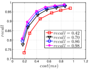
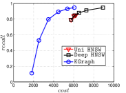
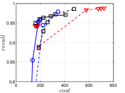
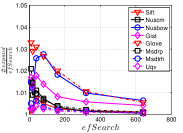
Since computing the exact KNNG requires huge cost in practice, researchers focused on the approximate KNNG to balance efficiency and accuracy. In practice, an accurate KNNG is urgent, because its accuracy will affect the downstream applications. Let us take DPG [17], an ANN search method, as an example. We conduct ANN search with DPG on two widely-used data sets, i.e., Sift and Gist, whose details could be found in Section 3.5, and show the results in Figure 1. As KNNG’s accuracy increases, DPG’s performance is obviously enhanced, where less cost leads to more accurate results.
During the past decade, a few approximate methods [6, 34, 36, 29] have been proposed. In general, they follow the same framework that quickly constructs an initial KNNG with low or moderate accuracy and then refines it by neighborhood propagation. Existing methods usually employ some index structures to construt the initial KNNG, including binary partition tree [6, 34], random projection tree [29] and locality sensitive hashing [36]. For neighborhood propagation, existing methods follow the same principle “a neighbor of my neighbor is also likely to be my neighbor” [9], despite some variations in technical details. In the rest of this paper, we denote the first step of constructing an initial KNNG as INIT and the second step of neighborhood propagation as NBPG.
Given the current research outcomes on KNNG construction in the literature, there remain several questions to be answered. First, it lacks a comprehensive experimental comparison among representative solutions in the literature. This may be caused by the fact that these authors come from different research communities (e.g., data mining, computer vision, machine learning, etc.) and are not familiar with some other works. Second, some related techniques in the literature have not been considered for the purpose of KNNG construction, such as SW graph [21] and HNSW [22], which are the state-of-the-art methods for ANN search. It remains a question whether they are potentially suitable methods for KNNG construction. Third, NBPG methods are effective on some data but not so effective on some other data. The relationship between the effectiveness of NBPG and data property is not clear yet.
To address the above issues, we revisit existing methods and make a comprehensive experimental study for both INIT and NBPG steps, to understand the strengths and limitations of different methods and provide deeper insights for users. In addition to existing methods for the INIT step, we adopt two related techniques for ANN search, i.e., SW and HNSW, as alternative methods for INIT, denoted as SW KNNG and HNSW KNNG respectively. Through our extensive experiments, we first recommend HNSW KNNG for INIT.
We categorize NBPG methods into three categories, i.e., UniProp [6, 36, 29], BiProp [9] and DeepSearch [34]. Both UniProp and BiProp adopt the iterative approach to refine the initial KNNG step by step. But UniProp only considers nearest neighbors in NBPG, while BiProp considers both nearest neighbors and reverse nearest neighbors. In contrast, DeepSearch runs for only one iteration, which conducts ANN search on an online rapidly-built proximity graph, e.g., the initial KNNG in [34] or the HNSW graph as pointed out in this paper. According to our experimental results, there is no dominator in all cases. But, we do not recommend the popular UniProp, because it usually cannot achieve a high-accuracy KNNG and is sensitive to . KGraph 111As an improved implementation of [9], it does not appear in the experiments of several existing works [6, 34, 36, 29], a variant of BiProp, has the best performance to construct a high-accuracy KNNG, but requires much more memory than other methods. Deep HNSW, a new combination under the framework, presents the best balance among efficiency, accuracy and memory requirement in most cases.
Besides the experimental study, we further investigate the effectiveness of NBPG versus data property. We employ the definition of node hubness in [24] to characterize each node, where the node hubness of a node is defined as the number of its exact reverse KNNs. Further, we extend this definition and define the data hubness of a data set as the normalized sum of the largest node hubness of its top nodes up to a specified percentage, in order to characterize the data set. With those two definitions in our analyses, we have two interesting findings. First, a high hub data usually has worse NBPG performance than a low hub data. Second, a high hub node usually has higher accuracy of their KNNs than a low hub ndoe.
We summarize our contributions as follows.
-
•
We revisit the framework of constructing KNNG and introduce new methods or combinations following it.
-
•
We conduct a comprehensive experimental comparison among representative solutions and provide our practical suggestions.
-
•
We investigate the effectiveness of NBPG and discover the strong correlation between its performance and the hubness phenomenon.
The rest of this paper is organized as follows. In Section 2, we define the problem and show the framework. In Section 3, we present INIT methods and conduct experimental evaluations on INIT. In Section 4, we describe various NBPG methods and show our experimental results. In Section 5, we investigate the effectiveness of NBPG mechanism and present our insights. In Section 6, we discuss related work. Finally, we conclude this paper in Section 7.
2 Overview of KNNG Construction
2.1 Problem Definition
Let be a data set that consists of -dimensional real vectors. The KNNG on is defined as follows.
Definition 1
[KNNG]. Given and a positive integer , let be the KNNG of , where is the node set and is the edge set. Each node uniquely represents a vector in . A directed edge exists iff is one of ’s KNNs in .
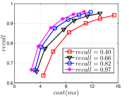
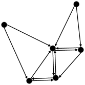
The KNNG of a data set with 6 data points is shown in Figure 2. For each node, it has two out-going edges pointing to its 2NNs. For simplicity, we refer to approximate KNNG as KNNG and approximate KNNs as KNNs in the rest of the paper. When we refer to exact KNNG and exact KNNs, we will mention them explicitly.
In this paper, we focus on in-memory solutions on high-dimensional dense vectors with the Euclidean distance as the distance measure, which is the most popular setting in the literature. This setting makes us focus on the comprehensive comparison on existing works. We would solve this problem with other settings, e.g., disk-based solutions, sparse data and other distance measures, in future works.
2.2 The Framework of KNNG Construction
Algorithm 1 shows the framework of KNNG construction, adopted by many methods in the literature [6, 34, 36, 29]. This framework contains two steps, i.e., INIT and NBPG. The philosophy of this framework is that INIT geneartes an initial KNNG quickly, and then NBPG efficiently refines it, which follows the principle “a neighbor of my neighbor is also likely to be my neighbor” [9]. Note that we do not expect INIT costs a lot for high accuracy, because the refinement will be done in NBPG.
In this paper, we will introduce a few representative approaches for INIT and NBPG respectively. For each method, we also analyze its memory requirement and time complexity. For memory requirement, we only count the auxiliary data structures of each method, ignoring the common structures, i.e., the data and the KNNG .
2.3 KNNG vs Proximity Graph
Proximity graphs (e.g., SW [21], HNSW [22], DPG [17] and NSG [10]) are the state-of-the-art methods for ANN search. Like KNNG, they treat each point as a graph node, but have distinct strategies to define ’s edges. The relationship between KNNG and proximity graph is twisted. On one hand, KNNG could be treated as a special type of proximity graph. Hence, KNNG is used for ANN search in recent benchmarks [2, 1, 17]. In those benchmarks, KNNG is usually denoted as KGraph, which is actually a KNNG construction method [9]. On the other hand, some proximity graphs such as DPG and NSG require an accurate KNNG as the premise, so that their construction cost is higher than KNNG. However, SW and HNSW are not built on top of KNNG and thus may be built faster than KNNG with adequate settings. As a new perspective, we show that SW and HNSW could also be used to build KNNG.
Moreover, we show ANN search on a proximity graph in Algorithm 2, which will be discussed more than once in this paper. Its core idea is similar to NBPG, i.e., “a neighbor of my neighbor is also likely to be my neighbor”. Let be a proximity graph and be a query. The search starts on specified or randomly-selected node(s) , which are first pushed into candidate set (a sorted node list). Let be the size of . In each iteration in Line 4-11, we find the first unexpanded node in and then expand in Lines 6-10, denoted as . This expansion treats each neighbor of on as a candidate to refine in Line 8-10, which is denoted as . Once the first nodes in have been expanded, the search process terminates and returns the first nodes in . Obviously, is key to the search performance. A large increases both the cost and the accuracy.
3 Constructing Initial Graphs
In this section, we introduce several representative methods for INIT. They can be classified into two broad categories: the partition-based approach and the small world based approach. The main idea of the former is to partition the data points into sufficiently small but intra-similar groups. Then each point finds its KNNs in the most promising group(s) and an initial KNNG is generated. The partition-based approach includes Multiple Division [34], LSH KNNG [36], and LargeVis [29]. These methods adopt different partitioning techniques. The main idea of the small world based approach is to create a navigable small world graph among the data points in a greedy manner, the structure of which is helpful for identifying the KNNs of any data point. The small world based approach was proposed to process ANN search in the literature, but not for KNNG construction. But we find it is trivial to extend them for KNNG construction. So we include these techniques in our study, which are denoted as SW KNNG [21] and HNSW KNNG [22]. We conduct extensive experiments to test and compare these methods for INIT.
3.1 Multiple Random Division
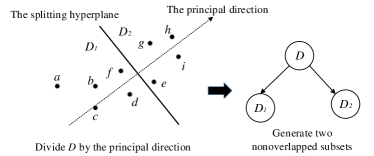
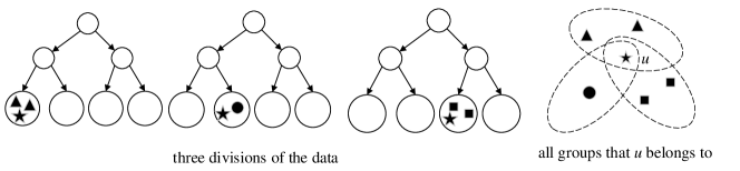
Wang et al. [34] proposed a multiple random divide-and-conquer approach to build base approximate neighborhood graphs and then ensemble them together to obtain an initial KNNG. Their method, which we denote as Multiple Division, recursively partitions the data points in into two disjoint groups. To assign nearby points to the same group, the partitioning is done along the principal direction, which could be rapidly generated [34]. The data set is partitioned into two disjoint groups and (as illustrating in Figure 3), which are further split in a recursive manner until the group to be split contains at most points. Then a neighborhood subgraph for each finally-generated group is built in a brute-force manner, which costs .
A single division as described above yields a base approximate neighborhood graph containing a series of isolated subgraphs, and it is unable to connect a point with its closer neighbors lying in different subgraphs. Thus, Multiple Division uses random divisions. Rather than computing the principal direction from the whole group, Multiple Division computes it over a random sample of the group. For each point , it has a set of KNNs from each division and thus totally sets of KNNs, from which the best KNNs are generated. We illustrate this process in Figure 4.
Cost Analysis: Since those divisions could be generated independently, the memory requirement is to store the current division. For each division, the recursive partition costs and the brute-force procedure on all finally-generated groups requires . With divisions, the cost of Multiple Division is . We can see that and are key to the cost of Multiple Division.
3.2 LSH KNNG
Zhang et al. [36] proposed a method, denoted as LSH KNNG, which uses the locality sensitive hashing (LSH) technique to divide into groups with equal size, and then builds a neighborhood graph on each group using the brute-force method. To enhance the accuracy, similar to Multiple Division, divisions are created to build base approximate neighborhood graphs, which are then combined to generate an initial KNNG of higher accuracy.
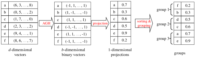
The details of such a division are illustrated in Figure 5. For each -dimensional vector, LSH KNNG uses Anchor Graph Hashing (AGH) [18], an LSH technique, to embed it into a binary vector in . Then, the binary vector is transferred to a one-dimensional projection on a random vector in . All points in are sorted in the ascending order of their one-dimensional projections and then divided into equal-size disjoint groups accordingly. Let be the size of such a group. Then a neighborhood graph is built on each group in the brute-force manner.
Cost Analysis: Like Multiple Division, each LSH division could be built independently. Hence, its memory requirement is caused by the binary codes and the division result. In total, its memory requirement is . In each division, generating binary codes costs and the brute-force procedure on all groups costs . In total, the cost of LSH KNNG is . We can see that the cost of LSH KNNG is sensitive to and , since is usually a fixed value.
3.3 LargeVis
Tang et al. [29] proposed a method, denoted as LargeVis, to construct a KNNG for the purpose of visualizing large-scale and high-dimensional data. Like Multiple Division, LargeVis recursively partitions the data points in into two small groups, but the partitioning is along a random projection (RP) that connects two randomly-sampled points from the group to be split. The partitioning results are organized as a tree called RP tree [7]. Similar to Multiple Division, RP trees will be built to enhance the accuracy. An initial KNNG is thus generated by conducting a KNN search procedure for each point on those trees. Each search process will be terminated after retrieving candidates 222Summarized according to the public codes from the authors https://github.com/lferry007/LargeVis. .
Cost Analysis: Unlike Multiple Division and LSH KNNG, we have to store all RP trees in the memory, since ANN search for each point is done on those trees simultaneously. Each tree requires space, since each inner node stores a random projection vector. Hence, the total memory requirement is . For each query, its main cost is to reach the leaf node from the root node in each tree and then verify candidates. Hence, the total cost of LargeVis is . We can see that and are key to the cost of LargeVis.
3.4 Small World based Approach
SW graph [21] and HNSW graph [22] are the state-of-the-art methods for ANN search [1, 17]. In the literature, neither technique (SW or HNSW) has been used for INIT. According to their working mechanism, it is trivial to extend them for INIT, while it needs a thorough comparison with other INIT methods in the literature.
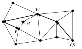
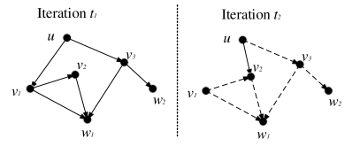
The SW graph construction process starts from an empty graph, and iteratively inserts each data point into . In each insertion, we first treat as a new node and then conduct ANN search as in Algorithm 2, where is the current SW graph and contains only a part of . Afterwards, undirected edges are created between and neighbors in . Figure 6 illustrates the insertion process for a data point . It is easy to generate an initial KNNG during the construction of . Before building , each point’s KNN set is initialized as empty. When inserting , its similar candidates will be retrieved by the search process and a distance is computed between and each candidate . We use (resp. ) to refine the KNN set of (resp. ). Once the SW graph is constructed, an initial KNNG is also generated. For simplicity, this method is denoted as SW KNNG.
Cost Analysis : The main memory requirement of SW KNNG is to store the SW graph, which needs space. Its main cost is to insert nodes. By experiments, we find that each insertion expands nodes, as demonstrated in Appendix A. But, there is no explicit upper bound on the neighborhood size. Let 333 is specific w.r.t. the data set, which is obviously affected by the hubness phenomenon as discussed in Section 5.1 be maximum neighborhood size in . In the worst case, its time complexity is .
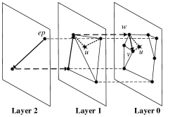
The HNSW garph is a hierarchical structure of multiple layers. A higher layer contains fewer data points and layer 0 contains all data points in . To insert a new point , an integer maximum layer is randomly selected so that will appear in layers 0 to . To insert , the search process starts from the entry point in the highest layer. The nearest node found in the current layer will serve as the entry point of search in the next layer, and this search process repeats in the next layer till layer 0. Note that the search in each layer follows Algorithm 2. After the search, HNSW creates undirected edges between and neighbors selected from returned ones, which is done in layers from to layer 0 respectively. Unlike SW, HNSW imposes a threshold on the neighborhood size. Once the edges of a node exceeds , HNSW prunes them by a link diversification strategy. Figure 7 illustrates an insertion in HNSW. By the same process in SW KNNG, we build the initial KNNG by tracing each pair of distance computation when building the HNSW graph. We denote this method as HNSW KNNG.
Cost Analysis: The main requirement of HNSW KNNG is caused by the HNSW graph, which contains nodes and each node has up to neighbors. Hence, its memory requirement is . The cost of HNSW KNNG mainly contains two parts, i.e., ANN search for each node and pruning operations for oversize nodes. We find that each search expands nodes as demonstrated in Appendix B and thus the total cost for ANN search is . Each pruning operation costs , but the exact number of those operations is unknown in advance. In the worst case, adding each undirected edge will lead to a pruning operation. In this case, there are totally pruning operations. However, the practical number of pruning operations on real data is far smaller than , as shown in Appendix B. Overall, the total cost of HNSW KNNG is in the worst case.
3.5 Experimental Evaluation of INIT
3.5.1 Experimental Settings
We first describe the experimental settings in this paper, for both INIT methods and NBPG methods.
Data Sets. We use 8 real data sets with various sizes and dimensions from different domains, as listed in Table I. Sift444http://corpus-texmex.irisa.fr contains 1,000,000 128-dimensional SIFT vectors. Nuscm555http://lms.comp.nus.edu.sg/research/NUS-WIDE.htm consists of 269,648 225-dimensional block-wise color moments. Nusbow666http://lms.comp.nus.edu.sg/research/NUS-WIDE.htm has 269,648 500-dimensional bag of words based on SIFT descriptors. Gist777http://corpus-texmex.irisa.fr contains 1,000,000 960-dimensional Gist vectors. Glove888http://nlp.stanford.edu/projects/glove/ consists of 1,193,514 100-dimensional word features extracted from Tweets. Msdrp999http://www.ifs.tuwien.ac.at/mir/msd/download.html contains 994,185 1440-dimensional Rhythm Patterns extracted from the same number of contemporary popular music tracks. Msdtrh101010http://www.ifs.tuwien.ac.at/mir/msd/download.html contains 994,185 420-dimensional Temporal Rhythm Histograms extracted from the same number of contemporary popular music tracks. Uqv111111http://staff.itee.uq.edu.au/shenht/UQ_VIDEO/index.htm contains 3,305,525 256-dimensional feature vectors extracted from the keyframes of a video data set.
| Data | Space | Baseline | Domain | ||
| Sift | 1,000,000 | 128 | 488 | 6,115 | Image |
| Nuscm | 269,648 | 225 | 231 | 803 | Image |
| Nusbow | 269,648 | 500 | 514 | 1,850 | Image |
| Gist | 1,000,000 | 960 | 3,662 | 63,430 | Image |
| Glove | 1,193,514 | 100 | 455 | 6,648 | Text |
| Msdrp | 994,185 | 1,440 | 5,461 | 87,630 | Audio |
| Msdrth | 994,185 | 420 | 1,593 | 24,053 | Audio |
| Uqv | 3,305,525 | 256 | 3,228 | 178,089 | Video |
Performance Indicators. We estimate the performance each method in three factors, i.e., cost, accuracy and memory requirement. We use the execution time to measure the construction cost, denoted as . The accuracy is measured by . Given a KNNG , let be the KNNs of from , and be its exact KNNs. Then . The of is averaged over all nodes in . The memory requirement is estimated by the memory space occupied by the auxiliary structures of each method. By default, is set to be 20 in this paper.
Computing Environments. All experiments are conducted on a workstation with Intel(R) Xeon(R) E5-2697 CPU and 512 GB memory. The codes are implemented by C++ and compiled by g++4.8 with -O3 option. We shut down the SIMD instructions to make a fair competition, since some public codes are implemented without opening those instructions. We run those methods in parallel 121212We do this due to two reasons. First, all the methods are easy to be executed in parallel. Second, there are many experiments in this paper. and the number of threads is set to be 16 by default.
3.5.2 Compared Methods and Parameter Selection
We evaluate the five methods described in this section. As listed below, their parameters are carefully selected following the goal, i.e., generating rapidly an initial KNNG with low or moderate accuracy in INIT. Note that the refinement will be done in NBPG.
-
•
Multiple Division : , as in [34], and (10 by default) is varied in .
-
•
LSH KNNG : , optimized by experiments, and is varied in .
-
•
LargeVis : we vary (50 by default) in and use default settings for others.
-
•
SW KNNG : and is varied in .
-
•
HNSW KNNG : , optimized by experiments, and (80 by default) is varied in .
Moreover, we use the brute-force method as the baseline method, which leads to distance computations. We list the cost of the baseline method in Table I.
3.5.3 Experimental Results

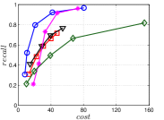
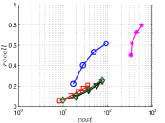
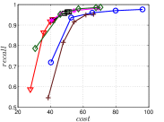
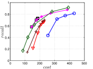
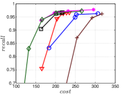
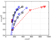
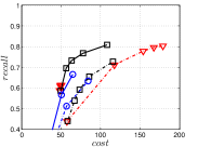
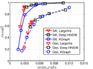
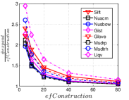
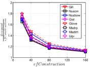
A good INIT method should have a good balance between and . We show the experimental results of vs in Figure 8. We can see that small world based approaches obviously outperform existing methods that employ traditional index structures. Compared with SW KNNG, HNSW KNNG presents stable balance bwetween and . We notice that on data such as Nusbow, Glove and Msdrp, SW KNNG presents high accuracy and high cost. As mentioned previously, this is not the purpose of INIT. By the way, we believe that it is caused by the hubness phenomenon as discussed later in Section 5.1.
Multiple Division performs better than LargeVis and LSH KNNG. This superior performance may be brought by the principal direction based projection, which is more effective than LSH functions and random projections for data partitioning. On Nusbow, Msdtrh and Uqv, LSH KNNG fails to construct a KNNG due to runtime errors in computing the eigenvectors when training the AGH model.
We show the memory requirement of auxiliary data structures of INIT methods with their default settings in Table II. We can see that LargeVis requires the most memory space due to storing 50 RP trees, followed by HNSW KNNG and SW KNNG that need to store an HNSW graph and SW graph repressively. Due to the independence of multiple divisions, Multiple Division and LSH KNNG only store the structures for one division in the memory and thus require obviously less memory.
| Data | Multiple Division | LSH KNNG | Large Vis | SW KNNG | HNSW KNNG |
| Sift | 7.7 | 30.5 | 722 | 164 | 180 |
| Nuscm | 2.3 | 8.2 | 243 | 44 | 49 |
| Nusbow | 3.2 | 8.2 | 329 | 44 | 49 |
| Gist | 11.3 | 30.5 | 874 | 164 | 179 |
| Glvoe | 9.2 | 36.4 | 1,208 | 196 | 215 |
| Msdrp | 16 | 30.3 | 1,013 | 163 | 179 |
| Msdtrh | 8.4 | 30.3 | 881 | 163 | 179 |
| Uqv | 25.6 | 100.9 | 2,488 | 542 | 654 |
Summary. For INIT, we first recommend HNSW KNNG. This is because HNSW KNNG presents consistently superior performance over other competitors. Even though its memory requirement is the second largest, it is still acceptable, especially compared to the data space as shown in Table I. Our second recommendation is Multiple Division, which has good performance and requires little memory space. Without the information of the data hubness, we do not recommend SW KNNG, since the user may encounter huge cost to complete the task.
4 Neighborhood Propagation
In this section, we study the NBPG technique in the framework of KNNG construction, which is used to refine the initial KNNG. In general, all methods in the literature follow the same principle: “a neighbor of my neighbor is also likely to be my neighbor” [9], but differ in the technical details. We categorize them into three categories: UniProp [36, 29], BiProp [9] and DeepSearch [34], and describe their core ideas as follows.
4.1 UniProp
As a popular NBPG method, UniProp stands for uni-directional propagation, which iteratively refines a node’s KNNs from the KNNs of its KNNs [36, 29]. Let be the KNNs of found in iteration . We can obtain from the initial KNNG constructed in the INIT step. Algorithm 3 shows how to iteratively refine the KNNs of each node. In iteration , we initially set as and then conduct (as in Algorithm 2) for each . UniProp repeats for times and terminates.
Cost Analysis: UniProp needs to store the last-iteration KNNG. Hence its space requirement is . Its time complexity is in the worst case.
4.2 BiProp
In contrast to UniProp, another type of method considers both the nearest neighbors and the reverse nearest neighbors of a node for neighborhood propagation [9]. Thus we denote it as BiProp which stands for bi-directional propagation. For each node , BiProp maintains a larger neighborhood with size , which contains ’s nearest neighbors found so far. BiProp also takes an iterative strategy. Let be the nearest neighbors of in iteration , where is a variable and does not necessarily equal to . Note that . We use to denote ’s reverse neighbor set and thus . Then we denote the candidate set for neighborhood propagation as:
We show the procedure of BiProp in Algorithm 4. is initialized randomly, and so is . In iteration , a brute-force search is conducted on for each , as in Lines 4 to 9. At the end of each iteration, BiProp will update and in Lines 10 and 11.
In practice, the reverse neighbor set may have a large cardinality (e.g., tens of thousands or even more) for some . Processing such a super node in one iteration costs as high as . To address this issue, BiProp imposes a threshold on and the oversize sets will be reduced by random shuffle in each iteration.
Both NNDes131313As a well-known KNNG construction method, it is publicly available on https://code.google.com/archive/p/nndes. and KGraph141414It is publicly available on https://github.com/aaalgo/kgraph. It is well known as a method for ANN search, but ignored for KNNG construction. follows the idea of BiProp. Their key difference is how to set and . In NNDes, and for all nodes, which is specified in advance. As in KGraph, is a specified value, but varies with node and the iteration , denoted as . To determine , three rules must be satisfied simultaneously, summarized from the source codes. Let be a small value (e.g., 10).
-
•
Rule 1 : and .
-
•
Rule 2 : .
-
•
Rule 3 : increases, iff such that the brute-force search on refines .
Cost Analysis: In NNDes, we need to store and . Since and , the required memory is . Its time complexity is ) in the worst case. In KGraph, we need to store and for each . is bounded by and thus . Its memory requirement is , which could be large enough since is usually set as a large value (e.g., 100). Its time complexity is in the worst case, but it is very fast in practice due to the filters as discussed in Section 4.4.
4.3 DeepSearch
Wang et al. introduced the initial idea of DeepSearch [34], as shown in Algorithm 5. It follows the idea of ANN search on a proximity graph , created online before neighborhood propagation. For , it refines by conducting ANN search with staring nodes from the initial KNNG. Unlike UniProp and BiProp, DeepSearch runs only for one iteration.
The proximity graph is key to the performance of DeepSearch. An appropriate should satisfy two conditions. First, should be rapidly built, since it is built online. Second, should have good ANN search performance. is the initial KNNG built by Multiple Division in [34], denoted as DeepMdiv, which satisfies the first condition but fails for the second. Among existing proximity graphs, HNSW is a good choice of DeepSearch, which satisfies both conditions. We denote this method as Deep HNSW. Others such as DPG [17] and NSG [10] require an expensive modification on an online-built KNNG, which violates the first condition. Thus they are not suitable for DeepSearch. The construction cost of SW is unstable as shown in Section 3.5 and its ANN search performance is usually worse than other proximity graphs [17]. Hence SW is not suitable.
Cost Analysis: DeepSearch needs to store the proximity graph. Thus DeepMdiv requires and Deep HNSW needs . The cost of DeepSearch is determined by two factors, i.e. the number of expanded nodes and their neighborhood sizes. We find that both DeepMdiv and Deep HNSW expand nodes, as demonstrated in Appendix C. Each node on KNNG has neighbors and thus the cost of DeepMdiv is . Each node on the HNSW graph has at most edges and thus the cost of Deep HNSW is .
4.4 Optimizations
In NBPG, there exist repeated distance calculations for the same pair of points, which increases the computational cost. In this section, we discuss how to reduce such repeated computations which can be categorized into two sources: intra-iteration and inter-iteration.
In the left graph in Figure 9, is a neighbor of both and , which are the neighbors of . In the neighborhood propagation, the pair will be checked twice in the same iteration. Thus we call this case intra-iteration repetition. To avoid the intra-iteration repetition, we use a global filter, a bitmap of size in each iteration. indicates whether has been visited or not. Let us take UniProp as an example. Before line 4 in Algorithm 3, we initialize all elements as . Then we check for candidate before line 6. If is a new candidate, we conduct and mark as . Otherwise, is just ignored. The global filter is also applicable to BiProp and DeepSearch.
Inter-iteration repetitions refer to the repeated computation in different iterations. Consider the two iterations in Figure 9 in which the pair is considered twice. To avoid the inter-iteration repetition, we can use a local filter. Let us take UniProp as an example. For each neighbor , we assign it an attribute , which is set as at start. If is firstly added to as a new neighbor, its is , otherwise it is as an old neighbor. In Figure 9, we use the solid arrows to represent new KNN pairs and the dashed arrows for old KNN pairs. In iteration , is an old neighbor of and is an old neighbor of . Thus the pair has been considered in a previous iteration and should be ignored by . Note that the inter-iteration repetition cannot be completely avoided by the local filter. Consider finds via a new neighbor in iteration , which is a repeated computation from iteration . The local filter can also be used for BiProp, but is not necessary for DeepSearch with only one iteration.
According to our knowledge, the global filter has been widely used in existing studies, while the local filter has not. The filters will accelerate NBPG methods, but will not change the cost analysis in the worst case. On the other hand, they introduce new data structures and require more memory. The space required by the global filter is , while that by the local filter is determined by the neighborhood sizes. To be specific, UniProp and NNDes require , while KGraph needs . Since the local filter is attached to the neighbors, it will not change the final space complexity.
4.5 Experimental Evaluation of NBPG
We use the same experimental settings in Section 3.5.1.

4.5.1 Compared Methods and Parameter Selection
We compare 6 NBPG methods as listed in the following and carefully optimize their parameters for their best performance. Following the framework, NBPG is also combined with our first choice HNSW KNNG in INIT, i.e., where and by default. We just list the settings of key parameters as follows.
-
•
UniProp: LargeVis [29] 151515We improve the codes from the authors by adding the local filter to reduce inter-iteration repeated distance computations in UniProp. and Uni HNSW. LargeVis takes 50 RP trees to build the initial KNNG, while Uni HNSW uses HNSW KNNG. The number of iterations is varied from 0 to 4.
- •
-
•
DeepSearch: DeepMdiv [34] and Deep HNSW. in DeepSearch is set between 0 and 160. The number of random divisions is 10 in DeepMdiv .
4.5.2 Experimental Results
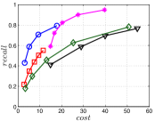
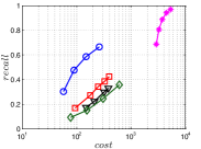
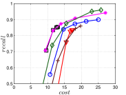
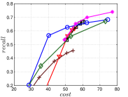
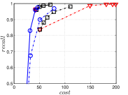
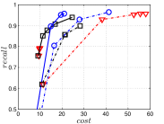
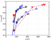
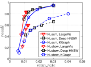
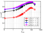
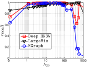
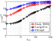
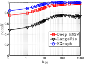
The experimental results of vs are plotted in Figure 10. We first compare the methods within each category. For UniProp, we can see that Uni HNSW obviously outperforms LargeVis in most cases, because Uni HNSW performs UniProp based on a better initial KNNG generated by HNSW KNNG. Notably, both methods have significant improvement in the first two iterations but rapidly converge afterwards. This is because most KNNs have become old neighbors in subsequent iterations and fewer candidates will be found for KNN refinement. For BiProp, KGraph obviously defeats NNDes. This is because NNDes fetches neighbors from a smaller neighbor pool in NBPG than KGraph. Moreover, KGraph carefully determines the neighborhood size and limits the size of for each in each iteration, to balance efficiency and accuracy. For DeepSearch, Deep HNSW is much better than DeepMdiv on all data sets except Nusbow, due to two reasons. First, HNSW KNNG outperforms Multiple Division in INIT. Second, the HNSW graph has much better performance on ANN search than KNNG, as demonstrated in recent benchmarks [1, 2, 17].
We list the memory requirement of auxiliary data structures of NBPG methods in Table III. We can see that KGraph requires the most memory for auxiliary structures, followed by NNDes. On the data with relatively small dimensions, such as Sift, Nuscm and Glove, KGraph even needs more space than the data itself. This is because KGraph maintains a large neighbor pool for each node and stores reverse neighbors. The space requirement of UniProp is mainly caused by the last-iteration KNNG, while Deep HNSW and DeepMdiv are due to their proximity graphs.
| Data | UniProp | NNDes | KGraph | Deep HNSW | Deep Mdiv |
| Sift | 97 | 332 | 1,158 | 181 | 78 |
| Nuscm | 26 | 90 | 309 | 49 | 21 |
| Nusbow | 26 | 90 | 318 | 49 | 21 |
| Gist | 97 | 332 | 1,177 | 180 | 78 |
| Glvoe | 115 | 396 | 1,346 | 216 | 93 |
| Msdrp | 96 | 330 | 1,101 | 180 | 77 |
| Msdtrh | 96 | 330 | 1,116 | 180 | 77 |
| Uqv | 319 | 1,098 | 3,644 | 657 | 256 |
Let us consider and compare all three categories of NBPG together. Overall, There is no denominator in all cases. Even with small memory requirement, UniProp usually cannot achieve high accuracy due to its fast convergence. KGraph is the best choice for a high-recall KNNG, but not for a moderate-recall KNNG. Besides, KGraph requires obviously more memory and thus is not suitable when the memory is not enough. We can see that Deep HNSW is the most balanced method, considering efficiency, accuracy and memory requirement simultaneously.
4.5.3 KGraph with an Initial KNNG
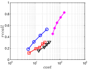
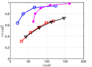
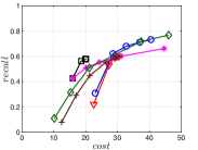
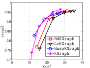
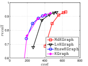
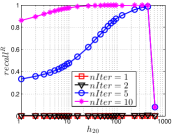
KGraph demonstrates impressive performance in the above experiments, but it starts from a random initial KNNG. Thus it is interesting to study the following question: How well can KGraph perform if we provide a good-quality initial KNNG? To answer this question, we create new combinations, LvKGraph, MdKGraph and HnswKGraph with three different initial KNNGs (i.e., LargeVis, Multiple Division and HNSW KNNG respectively) and then perform KGraph style of neighborhood propagation on top of these initial KNNGs. We show the results in Figure 11.

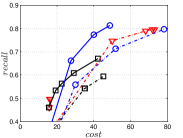
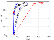
We can see that KGraph with a good-quality initial KNNG does not improve its performance. Even though HnswKGraph seems better than KGraph for a small or moderate , it is close to or even worse than KGraph when reaches a high value. Moreover, MdKGraph and LvKGraph are even worse than KGraph. This is caused by the fact that determining in KGraph is sensitive to the updates of KNNs according to Rule 3 in Section 4.2. When KGraph starts with an accurate KNNG, fewer updates happen in each iteration and thus fewer new neighbors will join in the next iteration. Moreover, there may exist repeated distance computations between INIT and KGraph, since some similar pairs may be computed repeatedly in these two steps.
4.5.4 Influences of
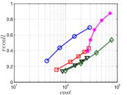
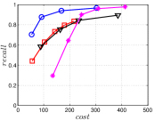
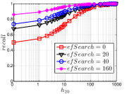
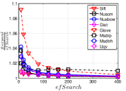
As a key parameter in NBPG, we study the influence of on three representative methods, i.e., Uni HNSW, Deep HNSW and KGraph. Here we select two values, i.e., a small value 5 and a large value 100, for each method. We show the results in Figure 13. We can see that has an obvious influence on Uni HNSW. With a large , its and increase significantly, while keeping almost unchanged with a small . This is because up to candidates will be found for each query in one iteration, which leads to larger and better . In addition, Uni HNSW is worse than its competitors for a large , except on Nusbow and Msdrp. As to Deep HNSW and KGraph, they have to pay more cost to achieve the same for a large , but they are not significantly affected by like Uni HNSW, because the way they find candidates is independent of .
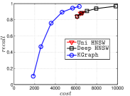
4.5.5 Performance on Large Data
To test the scalability of NBPG methods, we use two large-scale data sets, i.e., Sift100M 161616http://corpus-texmex.irisa.fr/ and Deep100M to evaluate the performance of three representative methods, i.e., Uni HNSW, KGraph and Deep HNSW. Sift100M contains 100 million 128-dimensional SIFT vectors, while Deep100M consists of 100 million 96-dimensional float vectors, which are randomly sampled from the learn set of Deep1B 171717https://yadi.sk/d/11eDCm7Dsn9GA. To deal with such large data, we set the number of threads as 48 for all three methods. We show the results on Figure 12. We can see that KGraph obviously outperforms Uni HNSW and Deep HNSW. This is because the construction of the HNSW graph costs quite a lot time, i.e., around 6,000 seconds for both data sets. Note that KGraph requires much more memory space than its competitors.
4.5.6 Summary
There is no dominator in all cases for KNNG construction. We do not reccommend UniProp, since it cannot achieve high accuracy due to its fast convergence and is pretty sensitive to . If the memory resource is enough and a high-recall KNNG is urgent, KGraph is the first choice. Otherwise, Deep HNSW is our first recommendation due to its superior balance among efficiency, accuracy and memory requirement.
| Low Hub | Moderate Hub | High Hub | ||||||
| Sift | Uqv | Msdtrh | Nuscm | Gist | Glove | Nusbow | Msdrp | |
| 0.007 | 0.014 | 0.012 | 0.036 | 0.039 | 0.075 | 0.066 | 0.259 | |
| 0.047 | 0.063 | 0.07 | 0.157 | 0.164 | 0.243 | 0.269 | 0.407 | |
| 0.285 | 0.319 | 0.355 | 0.531 | 0.549 | 0.647 | 0.694 | 0.740 | |
| 0.929 | 0.967 | 0.929 | 0.835 | 0.673 | 0.619 | 0.599 | 0.865 | |
| 0.992 | 0.982 | 0.991 | 0.942 | 0.874 | 0.786 | 0.661 | 0.879 | |
| 0.986 | 0.972 | 0.990 | 0.968 | 0.943 | 0.779 | 0.867 | 0.926 | |
5 Exploring Neighborhood Propagation
We are interested in the reasons why NBPG is effective. The principle (i.e., “a neighbor of my neighbor is also likely to be my neighbor” [9]) is intuitively correct and works effectively in practice, but it lacks convincing insights on its effectiveness in the literature. This motivates us to explore the NBPG mechanism. To achieve this goal, we employ the node hubness defined in [24] to characterize each node. Further, we develop this concept and propose the data hubness to characterize a data set. With those two definitions, we have two insights. First, the data hubness has a significant effect on the performance of NBPG. Second, the node hubness of a node has an obvious effect on its accuracy during the NBPG process. To present the effect of node hubness on its accuracy, we explore the dynamic process of three representative NBPG methods, i.e., LargeVis, KGraph and Deep HNSW, respectively.
5.1 Hubness and Accuracy of Reverse KNNs
According to [24], a hub node appears in the KNNs of many nodes, making it a popular exact KNN of other nodes. Accordingly, a hub node has a large in-degree in the exact KNNG. We show its definition from [24] as follows.
Definition 2
Node Hubness. Given a node and , we define its hubness, denoted as , as the number of its exact reverse KNNs, i.e., , where and represents the exact KNNs of .
According to [24], a hub node is usually close to the data center or the cluster center, and thus it is naturally attractive to other nodes as one of their exact KNNs. Further, we extend the hubness concept to the whole data set as follows.
Definition 3
Data Hubness. Given , and a percentage , we define the data hubness of at in Equation 1, where is a permutation of nodes in and is the node with the -th largest node hubness.
| (1) |
We can see that is actually the normalized sum of the largest values and thus is between 0 and 1. For the eight data sets, we divide them into three groups according to their data hubness, i.e., low hub, moderate hub and high hub respectively, as shown in Table IV. We can see that Msdrp has the largest data hubness, where the first (995) points have hubness (corresponding to over 5 million edges in the exact KNNG).
In addition, we define the accuracy of reverse KNNs. For a KNNG , we have as ’s reverse KNNs. Then we define the accuracy of ’s reverse KNNs as , where is defined as in Definition 2. reflects the accuracy of a KNNG to some extent, since a node probably has a high value on an accurate KNNG.
5.2 Effect of Data Hubness on NBPG Performance
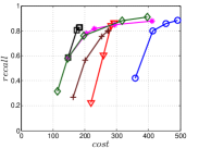
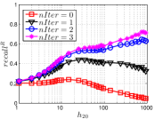
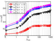
In this part, we present the effect of data hubness on the performance of NBPG. We discuss the performance in two aspects, i.e., (1) computational cost vs accuracy and (2) the converged accuracy. We use to measure the computational cost, where indicates the total number of distance computations during KNNG construction and is the number of all distance computations in the brute-force method. Unlike , is independent of . Here, we show the results on data size in Figure 14. We select data sets with the same size in each subfigure, so that we can focus on the effects of data hubness. We can see that the data hubness has a significant effect on the performance of NBPG methods. With a larger data hubess, each NBPG method has to compute more distances to achieve the same .
The converged is such a value that once an NBPG method reaches it, paying more cost cannot improve the value in a significant scale. We believe that the converged reflects the characteristic of an NBPG method. Here we obtain this value of a method by setting its parameters large enough. To be specific, the parameter settings are in LargeVis, in Deep HNSW and in KGraph. We show the results in Table 3. We can see that a lower hub data usually has a higher converged , while a higher hub data has a lower converged . This indicates that it is computationally expensive to get a high-recall KNNG for a high hub data.
5.3 Exploring UniProp
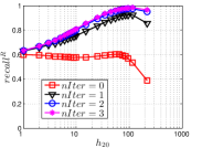
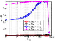
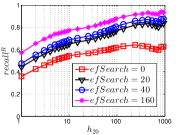
As a representative UniProp method, LargeVis starts from an initial KNNG with low or moderate accuracy and then conducts UniProp for a few iterations. Here we vary the number of iterations from 0 to 3. When , it corresponds to the initial KNNG. Due to the space limit, we only report the results on Sift and Glove in Figure 15. The -axis shows the node hubness of individual nodes and the -axis shows the or . We can see the values of all nodes increases substantially, especially in the first iteration. Notably, those newly found exact KNNs are mostly the hub nodes, as reflected by the significant increase in the values of hub nodes.
Even though the values of high hub nodes are not high in the beginning, as the cardinality of for these high hub nodes is large, there are still a good number of them that have been correctly connected to by many nodes as exact KNNs. Hence each node has a high chance to find those hub nodes via one of its KNNs in UniProp. That is why we observe a significant increase of in the first iteration. Overall, UniProp works well to find hub nodes as exact KNNs, but misses a significant part of non-hub nodes, which are less connected by other nodes and thus not easy to be found in UniProp. That is the reason why its converged recall (as shown in Table IV) is relatively low, especially on high hub data.
5.4 Exploring BiProp
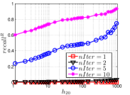
As a representative BiProp method, KGraph starts from a random initial graph and then conducts NBPG for a few iterations. Here we vary the number of iterations from 1 to 10. We show the results on Msdtrh and Nusbow in Figure 16. We can see that both and are pretty low in the first two iterations, due to the random initial graph. As KGraph continues, both and of high hub nodes increase obviously and approach almost the converged values in the fifth iteration. Unlike UniProp, and of moderate and low hub nodes obviously grow in later iterations. This is because KGraph conducts the brute-force search in , where each reverse neighbor (probably a non-hub node) will treat another reverse neighbor as a candidate. In other words, KGraph enhances the communications among non-hub nodes.
Notably, on Msdtrh, and are pretty low for some high hub nodes, whose values are larger than 400. This is caused by the fact that KGraph imposes a threshold on the number of reverse neighbors in order to ensure the efficiency. Hence the reverse neighbors of high hub nodes will be reduced, which has a negative influence on and of high hub nodes. But this loss could be made up by the increase in accuracy of non-hub nodes.
5.5 Exploring DeepSearch
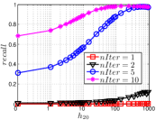
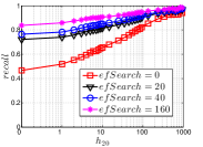
As a representative method of DeepSearch, the results of Deep HNSW are shown in Figure 17, where varies from 0 and 160. When , it corresponds to the initial KNNG, where both and of hub nodes are higher than those of non-hub nodes. Note that this is different from the initial KNNG generated by LargeVis, where hub nodes have even smaller values than non-hub nodes. This is because the construction of HNSW graph also employs the similar idea of NBPG that establishes the advantages of hub nodes in accuracy.
Like KGraph, and of non-hub nodes increase progressively in Deep HNSW as grows. DeepSearch enhances its accuracy by enlarging the expanded neighborhood for each node. As a result, more candidates will be found with a larger , which increases the chance of finding non-hub nodes.
5.6 Comparisons and Discussions
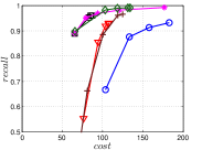
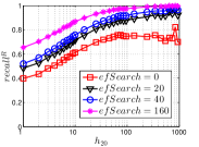
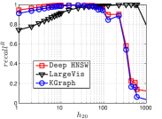
Now let us compare the converged accuracy of the three representative NBPG methods together. We show the results in Figure 18. On the low hub data set Uqv, it is interesting that both KGraph and Deep HNSW have small and for high hub nodes (i.e., ), while LargeVis has much larger values. This is because both KGraph and Deep HNSW limit the neighborhood size for each node . To be more detailed, KGraph limits the size of , while the HNSW graph limits the number of ’s edges. Since low hub data has a small number of hub nodes, it has a small impact on the overall . To some extent, this phenomenon reflects the preference of UniProp on hub nodes.
On the moderate hub data Gist, we can see the full advantages of KGraph in accuracy w.r.t. various hubness, followed by Deep HNSW and LargeVis. As indicated by the converged recall in Table IV, it will be more difficult to get high accuracy as the data hubness increases. The lower accuracy of LargeVis indicates that exploring the KNNs of each KNN does not work well for the low hub nodes of those difficult data, since UniProp obtains the candidates in the fixed neighborhood. To find more exact KNNs, we have to enlarge the neighborhood. Compared with LargeVis, Deep HNSW explores more than neighbors’ neighborhood on a fixed graph (i.e., the HNSW graph), while KGraph enlarges for each promising point iteratively. Moreover, they both use the reverse neighbors in the neighborhood propagation, which enhances the accuracy of non-hub nodes.
5.7 Summary
We find that the hubness phenomenon has a significant effect on NBPG performance in two aspects. First, there is a strong correlation between the data hubness and the performance of an NBPG method. We can expect a good balance between efficiency and accuracy and a good converged recall on a low hub data, while probably the opposite situation on a high hub data. Second, the node hubness significantly affects its accuracy in both and . We can expect a high hub node has a high and value, while a low hub node the opposite situation.
6 Related Work
Similarity search on high-dimensional data is another problem that is closely related to KNNG construction. Various index structures have been designed to accelerate similarity search. Tree structures were popular in early years and thus many trees [12, 5, 15, 26] have been proposed. Locality sensitive hashing (LSH) [14, 11] attracted a lot of attentions during the past decade, due to its good thorectical guarantee. Hence a few methods [20, 30, 19, 28, 13] based on LSH were created. Besides, there are also a few methods [27, 23, 16, 3, 4] based inverted index, which assigns similar points into the same inverted list and only accesses the most promising lists during the search procedure. Recently, proximity graphs [9, 21, 22, 17, 10] become more and more popular, due to their superior performance over other structures.
7 Conclusion
In this paper, we revisit existing studies of constructing KNNG on high-dimensional data. We start from the framework adopted by existing methods, which contains two steps, i.e., INIT and NBPG. We conduct a comprehensive experimental study on representative methods for each step respectively. According to our experimental results, KGraph has the best performance to construct a high-recall KNNG, but requires much more memory space. A new combination called Deep HSNW presents better balance among efficiency, accuracy and memory requirement than its competitors. Notably, the popular NBPG technique, UniProp, is not recommended, since it cannot achieve high-recall KNNG and is pretty sensitive to . Finally, we employ the hubness concepts to investigate the effectiveness of NBPG and have two interesting findings. First, the performance of NBPG is obviously affected by the data hubness. Second, the accuracy of each node is significantly influenced by its node hubness.
References
- [1] https://github.com/searchivarius/nmslib.
- [2] https://github.com/spotify/annoy.
- [3] A. Babenko and V. Lempitsky. The inverted multi-index. In CVPR, pages 3069–2076. IEEE, 2012.
- [4] D. Baranchuk, A. Babenko, and Y. Malkov. Revisiting the inverted indices for billion-scale approximate nearest neighbors. In ECCV, pages 202–216, 2018.
- [5] N. Beckmann, H.-P. Kriegel, R. Schneider, and B. Seeger. The R*-tree: an efficient and robust access method for points and rectangles. SIGMOD Record, 19(2):322–331, 1990.
- [6] J. Chen, H. R. Fang, and Y. Saad. Fast approximate knn graph construction for high dimensional data via recursive lanczos bisection. Journal of Machine Learning Research, 10(9):1989–2012, 2009.
- [7] S. Dasgupta and Y. Freund. Random projection trees and low dimensional manifolds. In STOC, pages 537–546. ACM, 2008.
- [8] C. Deng and W. Zhao. Fast k-means based on k-nn graph. In ICDE, pages 1220–1223. IEEE, 2018.
- [9] W. Dong, C. Moses, and K. Li. Efficient k-nearest neighbor graph construction for generic similarity measures. In WWW, pages 577–586. ACM, 2011.
- [10] C. Fu, C. Xiang, C. Wang, and D. Cai. Fast approximate nearest neighbor search with the navigating spreading-out graph. PVLDB, 12(5):461–474, 2019.
- [11] A. Gionis, P. Indyk, and R. Motwani. Similarity search in high dimensions via hashing. In VLDB, pages 518–529, 1999.
- [12] A. Guttman. R-trees: a dynamic index structure for spatial searching. In SIGMOD, pages 47–57. ACM, 1984.
- [13] Q. Huang, J. Feng, Y. Zhang, Q. Fang, and W. Ng. Query-aware locality-sensitive hashing for approximate nearest neighbor search. PVLDB, 9(1):1–12, 2016.
- [14] P. Indyk and R. Motwani. Approximate nearest neighbors: towards removing the curse of dimensionality. In STOC, pages 604–613. ACM, 1998.
- [15] H. V. Jagadish, B. C. Ooi, K. L. Tan, C. Yu, and R. Zhang. iDistance: an adaptive B+-tree based indexing method for nearest neighbor search. ACM Transactions on Database Systems, 30(2):364–397, 2005.
- [16] H. Jegou, M. Douze, and C. Schmid. Product quantization for nearest neighbor search. IEEE Transactions on Pattern Analysis and Machine Intelligence, 33(1):117–128, 2011.
- [17] W. Li, Y. Zhang, Y. Sun, W. Wang, M. Li, W. Zhang, and X. Lin. Approximate nearest neighbor search on high dimensional data – experiments, analyses, and improvement. IEEE Transactions on Knowledge and Data Engineering, 2019.
- [18] W. Liu, J. Wang, S. Kumar, and S. F. Chang. Hashing with graphs. In ICML, pages 1–8, 2011.
- [19] Y. Liu, J. Cui, Z. Huang, H. Li, and H. shen. SK-LSH : an efficient index structure for approximate nearest neighbor search. PVLDB, 7(9):745–756, 2014.
- [20] Q. Lv, W. Josephson, Z. Wang, M. Charikar, and K. Li. Multi-probe LSH: efficient indexing for high-dimensional similarity search. In VLDB, pages 950–961, 2007.
- [21] Y. Malkov, A. Ponomarenko, A. Logvinov, and V. Krylov. Approximate nearest neighbor algorithm based on navigable small world graphs. Information Systems, 45:61–68, 2014.
- [22] Y. Malkov and D. Yashunin. Efficient and robust approximate nearest neighbor search using hierarchical navigable small world graphs. IEEE Transactions on Pattern Analysis and Machine Intelligence, 2018.
- [23] J. Philbin, M. Isard, J. Sivic, and A. Zisserman. Lost in quantization: Improving particular object retrieval in large scale image databases. In CVPR, pages 1–8, 2008.
- [24] M. Radovanović, A. Nanopoulos, and M. Ivanović. Hubs in space: popular nearest neighbors in high-dimensional data. Journal of Machine Learning Research, 11(Sep):2487–2531, 2010.
- [25] S. T. Roweis and L. K. Saul. Nonlinear dimensionality reduction by locally linear embedding. Science, 290(5500):2323–2326, 2000.
- [26] C. Silpa-Anan and R. Hartley. Optimised KD-trees for fast image descriptor matching. In CVPR, pages 1–8. IEEE, 2008.
- [27] J. Sivic and A. Zisserman. Video google: A text retrieval approach to objects matching in videos. In ICCV, pages 1470–1478. IEEE, 2003.
- [28] Y. Sun, W. Wang, J. Qin, Y. Zhang, and X. Lin. SRS: Solving c-approximate nearest neighbor queries in high dimensional euclidean space with a tiny index. PVLDB, 8(1):1–12, 2015.
- [29] J. Tang, J. Liu, M. Zhang, and Q. Mei. Visualizing large-scale and high-dimensional data. In WWW, pages 287–297, 2016.
- [30] Y. Tao, K. Yi, C. Sheng, and P. Kalnis. Quality and efficiency in high dimensional nearest neighbor search. In SIGMOD, pages 563–576. ACM, 2009.
- [31] J. B. Tenenbaum, V. De Silva, and J. C. Langford. A global geometric framework for nonlinear dimensionality reduction. Science, 290(5500):2319–2323, 2000.
- [32] L. Van Der Maaten. Accelerating t-SNE using tree-based algorithms. The Journal of Machine Learning Research, 15(1):3221–3245, 2014.
- [33] J. Wang, J. Wang, Q. Ke, G. Zeng, and S. Li. Fast approximate k-means via cluster closures. In Multimedia Data Mining and Analytics, pages 373–395. Springer, 2015.
- [34] J. Wang, J. Wang, G. Zeng, Z. Tu, R. Gan, and S. Li. Scalable k-nn graph construction for visual descriptors. In CVPR, pages 1106–1113. IEEE, 2012.
- [35] W. Zhang, X. Wang, D. Zhao, and X. Tang. Graph degree linkage: Agglomerative clustering on a directed graph. In ECCV, pages 428–441, 2012.
- [36] Y. Zhang, K. Huang, G. Geng, and C. Liu. Fast knn graph construction with locality sensitive hashing. In ECML, pages 660–674. Springer, 2013.
![[Uncaptioned image]](https://cdn.awesomepapers.org/papers/ad2f4e6b-deda-4fae-82cc-5647aaf1a41b/x59.png) |
Yingfan Liu is currently a Lecturer in the School of Computer Science and Technology, Xidian University, China. He obtained his PhD degree in the department of Systems Engineering and Engineering Management of Chinese University of Hong Kong in 2019. His research interest contains the management of large-scale complex data and autonomous RDBMS. |
![[Uncaptioned image]](https://cdn.awesomepapers.org/papers/ad2f4e6b-deda-4fae-82cc-5647aaf1a41b/x60.png) |
Hong Cheng is an Associate Professor in the Department of Systems Engineering and Engineering Management at the Chinese University of Hong Kong. She received her Ph.D. degree from University of Illinois at Urbana-Champaign in 2008. Her research interests include data mining, database systems, and machine learning. She received research paper awards at ICDE’07, SIGKDD’06 and SIGKDD’05, and the certificate of recognition for the 2009 SIGKDD Doctoral Dissertation Award. She is a recipient of the 2010 Vice-Chancellor’s Exemplary Teaching Award at the Chinese University of Hong Kong. |
![[Uncaptioned image]](https://cdn.awesomepapers.org/papers/ad2f4e6b-deda-4fae-82cc-5647aaf1a41b/x61.png) |
Jiangtao Cui received the MS and PhD degrees both in computer science from Xidian University, China, in 2001 and 2005, respectively. Between 2007 and 2008, he was with the Data and Knowledge Engineering group working on high-dimensional indexing for large scale image retrieval, in the University of Queensland, Australia. He is currently a professor in the School of Computer Science and Technology, Xidian University, China. His current research interests include data and knowledge engineering, data security, and high-dimensional indexing. |
Appendix A The cost model of SW KNNG
The main cost of SW KNNG is to conduct ANN search for each . For each query , the search iteratively expands ’s close nodes until the termination condition is met. Hence we care about the number of expanded nodes for each query. To investigate it, we conduct experiments on real data. We show the results in Figure 19. We can see that as increases, the ratio decreases and becomes graudally close to 1. On average, we conclude that each query expands nodes. Unfortunately, nodes in an SW graph have various number of neighbors. Hence, we cannot figure out the number of candidates accessed precisely. Let the maximum neighborhood size in the SW graph. In the worst case, the time complexity of SW KNNG is .
Appendix B The cost model of HNSW KNNG
The main cost of HNSW KNNG contains two parts, i.e. ANN search for each node and pruning oversize nodes. Like SW KNNG, we find that the number of expanded nodes for each query is pretty close to . We show the relationship between the ratio and in Figure 20. We can see that the ratio approaches 1 as increases. Hence, we can conclude that each query expands nodes on average. Unlike an SW graph, each node in an HNSW graph has at most neighbors. Moreover, after each search, HNSW selects neighbors from ones, following the link diversification strategy like the pruning operations. Each such selection costs . In total, the part of ANN search for nodes costs .
Like , we investigate the number of pruning operations by experiments. We use the heuristic 2 (i.e., the default setting) in nmslib library as the link diversificaiton strategy, which generates fewer pruning operations. We show the experimental results in Figure 21. We can see that increases obviously as rises. However, we set as a small enough value (e.g., 80) in this paper. This is because we do not expect a pretty accurate KNNG for an INIT method. Hence, the practical will be sufficiently small.
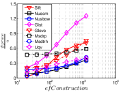
In addition, the data hubness (defined in Section 5.1) also has a positive influence on . Let us take Sift and Gist as an example. With the same value, Gist has an obvious than Sift. Similar phenomena could be found when comparing the pair of Nuscm and Nusbow and the pair of Msdrp and Msdtrh respectively. Moreover, the data size also positively affect . In Figure 22, we show the results on four subsets with sizes 1 million, 2 million, 4 million and 8 million of Sift100M, denoted as Sift1M, Sift2M, Sift4M and Sift8M respectively. The details of Sift100M could be found in Section 4.5.5.
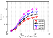
Even affected by a few factors, is pretty close to in practice, especially considering a small value. Hence, the practical values of are far smaller than the worst case , where in our experiments.
Appendix C The cost model of DeepSearch
DeepSearch conducts ANN search on a online-built proximity graph for each query . The search process is controlled by the parameter . The main cost of DeepSearch is to expand similar nodes to each query in . Hence, the number is key to the cost model of DeepSearch. Here, we investigate two variants of DeepSearch, i.e. DeepMdiv and Deep HNSW. We show relationship between and in Figure 23.
We can see that the ratio gradually approaches 1 as increases. We can say that DeepMdiv and Deep HNSW expand nodes for each query. DeepMdiv takes the initial KNNG as the proximity graph, where each node has exactly neighbors. As a result, the cost of DeepMidv is . Deep HNSW uses the HNSW graph as the proximity graph, where each node has up to neighbors. Hence, the cost of Deep HNSW is .