1 Department of Physics, Indian Institute of Technology Bombay, Mumbai, India
\affilTwo2 Department of Physics, University of Wisconsin-Milwaukee, Milwaukee, Wisconsin, USA
Revisiting the Earth’s atmospheric scattering of X-ray/–rays and its effect on space observation: Implication for GRB spectral analysis
Abstract
A considerable fraction of incident high energy photons from astrophysical transients such as Gamma Ray Bursts (GRBs) is Compton scattered by the Earth’s atmosphere. These photons, sometimes referred to as the “reflection component”, contribute to the signal detected by space-borne X-ray/–ray instruments. The effectiveness and reliability of source parameters such as position, flux, spectra and polarization, inferred by these instruments are therefore highly dependent on the accurate estimation of this scattered component. Current missions use dedicated response matrices to account for these effects. However, these databases are not readily adaptable for other missions, including many upcoming transient search and gravitational wave high-energy Electromagnetic counter part detectors. Furthermore, possible systematic effects in these complex simulations have not been thoroughly examined and verified in literature. We are in the process of investigation of the effect with a detailed Monte Carlo simulations in GEANT4 for a Low Earth Orbit (LEO) X-ray detector. Here, we discuss the outcome of our simulation in form of Atmospheric Response Matrix (ARM) and its implications of any systematic errors in the determination of source spectral characteristics. We intend to apply our results in data processing and analysis for AstroSat-CZTI observation of such sources in near future. Our simulation output and source codes will be made publicly available for use by the large number of upcoming high energy transient missions, as well as for scrutiny and systematic comparisons with other missions.
keywords:
GRB, Atmospheric scattering, X-ray, GEANT4souravspace@iitb.ac.in
12.3456/s78910-011-012-3 \artcitid#### \volnum000 0000 \pgrange1– \lpLABEL:LastPage
1 Introduction
X-ray/–ray astrophysical observations are primarily conducted from space-based platforms as the Earth’s atmosphere does not transmit these high energy photons. While most photons are absorbed, a fraction of the X-ray/–ray photons from any extra-terrestrial sources undergoes Compton scattering in the upper layers of the atmosphere. In the Earth’s atmosphere, which has a mass column density of at sea level, some of the scattered photons travel upwards having an appearence of reflection of X-ray/–ray by the atmosphere. Any space borne measurement of those high energy photons from astrophysical sources will be affected by simultaneous detection of the reflected photons.
The topic of interaction of extra-terrestrial high energy photons with the atmosphere is not new. Various studies have been performed to determine the spectrum of reflected Cosmic X-ray Background (CXB)111Alternately termed as Cosmic Diffused Gamma ray Background (CDGRB). photons from the Earth’s atmosphere and their effects on observations by various space-based high-energy instruments (e.g. Churazov ., 2008). Such works are often done in conjugation with studies determining the X-ray/–ray spectrum arising from the interaction of Cosmic ray particles (e.g. Sazonov ., 2007) with the molecules in Earth’s atmosphere. Together these two components constitute the X-ray/–ray albedo contribution and add up to the total background noise in high energy space detectors.
Apart from such studies in the context of Earth’s atmosphere, the main motivation of research related to the Compton reflection of high energy photons has been of purely astrophysical nature. This includes mainly the study of the scattering during the passage and interaction of cool electrons in relatively cooled plasma, such as the corona above a relatively cool, optically thick accretion disk (e.g. Bisnovatyi-Kogan & Blinnikov, 1977). In such studies one usually calculates a Green’s function describing the reflection of monochromatic radiation (White ., 1988), and convolves the incident spectrum with this function to calculate the reflected spectrum.
From the studies of Earth’s atmospheric scattering of high energy photons it is estimated that a moderate fraction of the incoming X-ray/–ray photons is reflected or back-scattered in the upper atmospheric layers of the Earth. Some studies estimate that in the 30 – 300 keV energy range (hereafter referred to as “intermediate energy”) of X-rays/–rays, as many as % of the incident photons can be scattered back (see for instance Churazov ., 2008). The scattered fraction decreases outside this energy range, but remains non-negligible over a much broader X-ray/–ray band.This suggests that Low Earth Orbit (LEO) satellites observing energetic photons from Gamma Ray Bursts (GRBs) and other astrophysical transients detect significant flux reflected from the Earth’s atmosphere as well. The magnitude and spectrum of the contribution should vary largely based on the relative angular position (viewing angle) of the GRB with respect to the instrument, as well as to the line joining the instrument to the geo-center, relative orientation of the instrument with the ground, and the source spectral properties. Whether this is considered as an interpretable addition to the source signal or merely as an addition to the background noise detected by the instrument like the CXB and albedo photons, any analysis of properties of the transients should correctly account for the contribution.
Till date, the contribution of Earth’s reflection of X-rays and –rays in prompt GRB observation has mainly been studied from the standpoint of its application in study of firstly, polarization in those wavelengths (e.g. Willis ., 2005) and secondly in the process of localization of transient source (e.g. Pendleton ., 1999). The fact that the angular distribution of Compton scattered flux from Earth’s atmosphere should be dependent on the direction of polarization of the incoming photon beam from a distant GRB sources, has been exploited to find the polarization characteristics from measurement of the reflected X-ray flux. There has been rigorous investigation (Pendleton ., 1999) for estimating the atmospheric scattering contribution to accurately determine transient source location by CGRO/BATSE and Fermi missions. They mainly concentrate on Monte Carlo simulation studies and some observations with solar flares.
We investigated how various missions have incorporated the Earth reflection effect in their data processing. We have been particularly interested in digging into the CGRO/BATSE and Fermi/GBM spectral data processing and distribution, as these two have been the main workhorses in providing the spectral observation of GRB prompt emission from hard X-rays up to soft –ray part of the spectrum. In case of CGRO/BATSE the atmospheric contribution is evaluated during burst localization using EGS electromagnetic cascade Monte Carlo code with a spherical geometry of concentric shells representing an atmosphere with exponential density. Subsequent iterative minimization technique is followed (Pendleton ., 1999) to differentiate the scattering contribution from the total observed spectra consisting of photons both directly detected from the source and those scattered from atmosphere.
The analyses presented by Pendleton . (1999) show us the extent to which the atmospheric scattering of source photons can contaminate observation of transients. In Figure 3 of the article demonstrating the distribution of number of GRBs detected by the detectors of different viewing angles (with respect to the burst) as function of the ratio of the detected atmospheric scattered flux to that of directly detected flux, it seems that for the detector with large viewing angles for a significant number of cases the detected scattered counts are well above the direct counts (by as much as an order). For moderate viewing angles the scattering rate is between 20% and 50% of that of the direct count rate. Figure 4 of the same article is also significant, depicting how the detected scattered to direct photon ratio can vary with zenith angle (i.e., the angle between the direction from instrument to the geo-center and the direction to the GRB), the viewing angle (w.r.t the burst) of detector and the orientation of the detector normal respective to the ground normal. The bottom-left plot showing the variation of the ratio with the source zenith angle for large viewing angle of the downward-facing detectors demonstrates the highest contribution of atmospheric scattering and its sharp dependence on photon incidence angle.
For Fermi/GBM, according to Meegan . (2009), the atmospheric scattering response estimation has been performed following the same method as described for BATSE in the GEANT4 based GBM Response Simulation System (GRESS; Hoover ., 2005; Kippen ., 2007) and validated with BATSE simulation results. This is then used to form a source-specific total response function for a particular set of earth-spacecraft viewing conditions, to be calculated in the IODA DRMGEN software in stand alone mode. Whereas, Connaughton . (2015) directly use the atmospheric response database established for BATSE (Pendleton ., 1999) in their study.
The problem of unwanted contribution of atmospheric scattering of X-ray/–ray is well addressed and steps have been followed to mitigate it, albeit, seemingly, there has been no quantitative, comprehensive and generalized description on how this should manifest in the estimation of the source characteristics, such as photon spectrum and polarization. These studies have been highly focused on specific instruments, and the final products are often deeply integrated with the instrument response function. Instead, in this work we take a generalized approach by concentrating on the Monte Carlo simulation of the interaction of energetic astrophysical source photon at atmosphere, completely devoid of any specific instrument interactions and characteristics. Thus, our goal is to calculate the distribution of atmospheric Compton scattered photons for a plane–parallel photon beam incident upon the Earth’s atmosphere and how it should manifest on the outcome of the spectral and polarization characteristics of the cumulative photon detection. Here we are presenting our findings only on the spectral front and intend to address the same on polarization elsewhere.
The broader goal of this work is two-fold. The first is to replicate the work that has been performed for other missions, and apply it directly to analysis of sources in AstroSat-CZTI (Singh ., 2014; Bhalerao ., 2017b; Rao ., 2017). Since its launch 5 years ago CZTI has detected more than 400 GRBs (Sharma ., 2020). CZTI has been used for some GRB localization studies (Bhalerao ., 2017a), and has also been very successful in detection of polarization in them (see Chattopadhyay ., 2019). Inclusion of the process of evaluation and deduction of atmospheric scattered contribution from prompt GRB spectra will be a significant step towards accurate analysis of all the above characteristics.
The second goal of the work is to publicly release all source codes and simulation data in a format that will be easy to adapt to any other mission. This goal stems from the plurality of upcoming and proposed missions to study high energy transients and gravitational wave high-energy electromagnetic counterpart detection, such as large instruments like SVOM (Cordier ., 2015), GECAM (Zhang ., 2019); as well as cubesat class instruments like BurstCube (Racusin ., 2017), HERMES (Fuschino ., 2019), BlackCAT (Chattopadhyay ., 2018), and Camelot (Werner ., 2018). There are also proposed missions, which are scientifically oriented towards hard X-ray/gammma ray polarimetry, such as POLAR-2 (Hulsman ., 2020) on-board Chinese space station and a Large Area GRB Polarimeter (LEAP) (McConnell ., 2017) on-board ISS. Rather than each of these missions developing their own atmospheric scattering databases, a single open database will serve the purpose well. It will also make it possible for comparisons between any other atmospheric scattering simulations, thus arriving at a quantitative estimate of systematic errors that may be present in the responses.
The organization of the paper is as follows. In Section 2, we discuss our simulation setup including detector geometry of Earth’s atmosphere and photon collecting detector, the physics of interaction and photon generation and run execution process. In Section 3 we presents our simulation outcome for mono-energetic photons and a hypothetical GRB spectrum, represented by Band function (Band ., 1993). In this section we will also investigate how the scattered photon contribution may change the spectral characteristics and possibly contribute artefacts in the exact evaluation of the spectral slope, if they are not accounted for correctly. We conclude in Section 4 by discussing about the outcome of our study and describing our future plan of work.
2 Monte Carlo simulation with GEANT4
We have used GEometry ANd Tracking 4 (GEANT4) for simulating the Compton reflection of X-rays from Earth’s atmosphere. GEANT4 is a well known Monte Carlo detector simulation package (Agostinelli ., 2003) written in C++, initially developed for the simulation of high energy physics and gradually got enhanced, in order to be applied to lower energies also. Currently, it is used extensively in high energy detector and instrument simulation (mass model) of most of the astronomical missions including AstroSat-CZTI (Mate ., 2021). Below we describe the construction of the simulation geometry including the Earth’s atmosphere, the generic detector at LEO height, the physics models used in the simulation, and the methods for particle generation, data extraction, and analysis.
2.1 Geometry and Earth’s atmosphere
The Monte Carlo code developed for this study primarily imitates the interactions of incident parallel mono-energetic beams of X-ray and –ray photons with Earth’s atmosphere and find the detection responses at an imaginary flat and fully efficient detector placed at LEO, at height of 650 km.
The attenuation of incoming X-ray to –ray photons in the atmosphere occurs predominantly from few 100s of km down to 10 km (see Palit ., 2018). About 99.7% of Compton back-scattering events occur below 125 km (Willis ., 2005), with the majority of the interactions occurring in the 20–50 km range. Considering this, we restrict the atmospheric heights from 10 km to 500 km in the simulation. The lower part of this range is of significantly varying density and concentration of neutral components. Those are mainly Nitrogen molecules (N2), Oxygen molecules (O2) and some other less abundant elements like Helium and Argon, which play an important role in the interaction process of high energy photons. Above km the mass column density of the atmosphere is below and the optical depth is so low that the variation in such concentration has negligible effect. Other than the inhomogeneity along vertical direction, the atmosphere also has inhomogeneities along latitude and longitude, and is dynamic in nature. For example, the atmosphere is thinner over the poles and thicker over the equator. Since our focus is on satellites in Equatorial orbits and we aim to calculate the nominal scattering effect, these are secondary concerns and can be neglected safely. In view of this we incorporated only vertical stratification in the atmosphere with the necessary data on density, and various neutral concentrations.
GEANT4 detector or geometry construction supports only concentric spherical shells. We model the Earth’s atmosphere using multiple layers in the detector construction class. The distribution of layers is as follows: The first ninety layers starting from 10 km above the Earth’s surface have a thickness of 1 km each, followed by 20 layers of 5 km each, and lastly the 12 outermost layers are of 25 km each. They are formed with average molecular densities and other atmospheric parameters at those heights. Corresponding neutral atmospheric data are obtained from NASA-MSISE-90 atmospheric model (Hedin, 1991). This atmospheric structure is directly imported from previous studies (Palit ., 2013, 2018), which already have successfully evaluated the X-ray interaction process though in the context of solar flares and their effect on radio propagation. A NaI detector disc of radius of 100 km and thickness of 10 meter (ensuring 100% absorption of received photons) is placed at a height of 650 km from the Earth’s surface at the zenith (direction, vertically upward from Earth’s centre). A schematic of the simulation geometry along with the photon generation and propagation through atmosphere has been presented in Figure 1.
2.2 Physics of interaction
The main interaction process for energetic photons corresponding to soft to hard X-rays and soft –rays with the atmospheric molecules are the primary photo-ionization and subsequent secondary electron ionization. The ionization can be due to photoelectric effect and Compton scattering. Electron-positron pair creation takes place for photon energies exceeding 1000 keV and has very small contribution in the overall interaction statistics. Due to the presence of a small amount of Helium and few other heavier elements in the Earth’s atmosphere The photoelectric cross section exceeds the scattering one up to energies 30 keV and inelastic (Rayleigh) scattering in atmospheric composition dominates the total scattering cross section at energies below 10–20 keV (Churazov ., 2008).
Each of the Physics processes in GEANT4 uses several models. Models for all electromagnetic processes can be subdivided into four general physics scenario categories: standard, low-energy, polarized and adjoint. For unpolarized low energy photons, most Compton scattering models corresponding to ‘low-energy’ and the ‘standard’ categories use the Klein-Nishina approach Klein & Nishina (1929) for cross-section. The other two efficient models (of ’low-energy’ category), namely, Livermore and Penelope based Compton scattering models use cross section calculation based on the EPDL data library (Cullen, 1995) and Penelope code (Sempau ., 2003). All these models, namely, the G4LivermoreComptonModel, G4PenelopeComptonModel, G4LowEPComptonModel etc. produce very similar outcome for our simulations. In the subsequent sections, we present the results computed with the G4PenelopeComptonModel and corresponding other Penelope low energy physics models.
2.3 Source photons, interactions and simulation steps
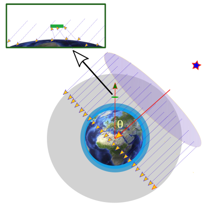
During source photon generation within primary generation class of GEANT4, an imaginary hollow sphere of large radius (7200 km) is assumed concentric to the Earth’s layered atmosphere. The photons are generated randomly on the surface of an imaginary flat disc (Figure 1) of same radius, touching the outer surface of the sphere at a point of intersection of the incoming photon direction with it and placed tangentially. This ensures that the photon incidence corresponds to plane wave coming from virtually infinite distance. During the simulation the detector is always kept at the vertically up-word position (zenith) that is on an imaginary vertical line extending upward from the center of the Earth. The angular position of the source () i.e., the incidence angle is always set with respect to the vertical line (Figure 1). corresponds to normal incidence on the atmosphere, with the detector directly between the source and the Earth. The detector is insensitive to direct source photons. The effect of the small shadow of the detector is corrected for by scaling up the observed counts to the unobstructed cross-section of the Earth.
We run each of our simulations with a mono-energetic photon beam having sufficient number () of photons, so that the detector can collect 10000 scattered photons from the whole of the atmosphere. Each run comprises of primary photons at a single energy. Our simulations span the energy range from 5 keV to 5 MeV as follows: 2 keV intervals from 10 to 50 keV, 5 keV intervals from 50 to 200 keV, 20 keV intervals from 200 to 400 keV, 100 keV intervals from 400 to 1000 keV, and simulations at 2000, 3000, 4000 and 5000 keV. This division is carefully chosen to get a smooth Atmospheric Response Matrix (ARM) (described in §3) by interpolation of the resultant mono-energetic distribution functions over incident energy values. Simulations are carried out for varying incidence angles (), and here we focus on a representative subset of these incidence angles. Details of the simulation steps and subsequent processing and analysis are covered in the §3.
3 Results
As discussed in the previous section, we undertake simulations only for mono-energetic beams with different incidence angles. The outcome, with suitable interpolation can easily be converted into response matrix and the spectrum for any realistic astrophysical source has to be synthesized by using a weighted sum of the simulated mono-energetic responses. The weights are to be determined by the number of source photons expected at that incident energy. The exercise of starting with mono-energetic incident beams has two main advantages. Firstly, it is helpful in better understanding of the exact nature of the atmospheric scattering response and how it varies over the incident photons at different ranges of X-ray/–ray energies. Secondly, this allows us to re-use our simulation results for any incident spectrum, without resorting to computationally expensive runs for each of them.
3.1 Mono-energetic response and Atmospheric Response Matrix (ARM)
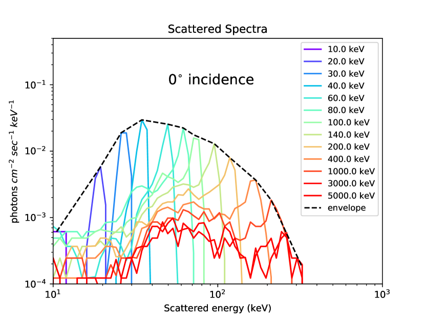
Figure 2 shows the detected (simulated) atmospheric scattered spectra for few of the incident energies, normalized for a single incident photon at that energy. The incidence angle () for this plot is 0∘. Due to inelastic interactions, many source photons get scattered to lower energies, creating a broadband spectrum for each of the mono-energetic incident photons. The maximum energy of scattered photons, as well as the energy at which the scattered spectrum peaks, are both below the incident energy. Both the parameters increase with the incidence beam energy up to few hundreds of keVs, but as incidence energy goes higher and crosses 1 MeV the maximum and peak energies of scattered photons stop increasing. We found that whatever higher the incident energy values are used, the energies of scattered photons remain well below 1 MeV. The maximum value of the scattering response peak occurs for incidence photon energy of 40 keV and lies at detected energy of 35 keV. Note that this maximum refers only to the peak in the observed spectrum, and not the total number of detected photons. The response diminishes as one goes from lower incidence angles to higher ones.
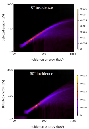
In Figure 3, the detected atmospheric responses to incidence photons of different energies are demonstrated for two different angles of incidence with values represented by the color bars. The -axis corresponds to the energy of the incident photons, while the -axis denotes the energy of scattered photons. The color coding shows the intensity at each energy pair. It is obvious that the detected energy is never greater than the incident energy, leaving the upper left part of these figures blank. These plots represent the ARM for various incidence angles, and the curves shown in Figure 2 correspond to horizontal slices through the plot in top panel of Figure 3. Values for incident energies other than those used in our simulation grid are obtained by suitable interpolation.
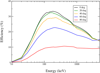
For each energy of incidence, we calculate the area under the scattering response curve (Figure 2) to obtain the atmospheric scattering efficiency, i.e., the total number of scattered photons (at any possible scattered energy) for a single incident photon on Earth’s atmosphere. We converted this in percentage and plot in Figure 4 as function of incidence energy for various incidence angles. The plots show that the scattering efficiency is maximum for 0∘ incidence of photons (black curve) and diminishes as the angle of incidence increases. For normal incidence the highest efficiency is at keV, and as Figure 2 shows, these photons are spread over a broad band of lower energies. The energy at which the atmospheric scattering efficiency is highest tends to gradually increase until the efficiency profile becomes nearly uniform in all energies above 100 keV for large incidence angles.
3.2 Spectral response for GRBs
We now discuss the scattering response of the Earth’s atmosphere to an incident GRB spectrum, approximated by a typical Band function (Band ., 1993). The parameters of the Band function given by Wanderman & Piran (2015) corresponding to a typical short GRB, viz, , , and keV are chosen for the calculation. The scattered component corresponding to the spectrum for 0∘incidence is estimated by the convolution of the spectrum with the corresponding response matrix (ARM representing the atmospheric scattering in top of the Figure 3). We pick the norm for the band function such that the fluence of the GRB is (20-200 keV) over 1 sec interval of prominence.
In order to disentangle the effects of the ARM from any instrument response effects, we assume that the instrument is an ideal omnidirectional detector: it measures the exact energy of each incident photon, but cannot discern photon incidence directions. In actual analysis of course, the direction- and energy-dependent response of the instrument would have to be folded into the calculation.
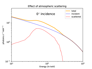
Simulation results for the atmospheric scattering component is shown in the upper panel of Figure 5. The dashed blue curve is the incident band spectrum, that would be detected directly, and the dashed red curve shows the scattered component from the atmosphere. The solid orange curve represents the net detected spectrum by a detector in LEO. We can see that a significant amount of photons scattered by the atmosphere are detected at the intermediate energy range of 30–300 keV. This reflected component produces a broad hump around 60 keV on top of the direct Band spectrum.
| Energy range (keV) | Flux ratio |
|---|---|
| 50 – 100 | 0.66 |
| 100 – 200 | 0.46 |
| 200 – 400 | 0.08 |
| 400 – 1000 | 0.001 |
| 20 – 2000 | 0.25 |
In Table 1 we show the ratio of the detected scattered flux from atmosphere to that of the incident flux integrated over various energy ranges for the Band function corresponding to the GRB used in our study. We see that the number of reflected photons in the 50–100 keV range is as high as 66% of the incident photons, which corresponds to of the total observed photon counts in this energy range.
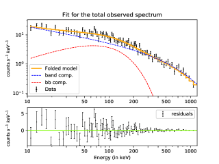
At a glance, the scattered component mimics a blackbody component (Figure 5, Top panel), and would have to be modelled so, if atmospheric scattering effects were not accounted for. As an illustration, we show such a naive analysis where the net observed spectrum can indeed be fit well by a Band + blackbody spectral model (Figure 5: Bottom panel).
To undertake formal fits we simulate an “observed” spectrum consisting of the direct incident and reflected spectra. The GEANT4 output is binned at 1 keV resolution, and multiplied by the effective area of the detector to obtain the expected count rate (in units of counts keV-1) as a function of energy. To account for Poisson noise, we calculate the final observed number of photons in each 1 keV by using a Poisson distribution with rate equal to . The uncertainty for each bin is set to . We note that in practice, the uncertainties will be higher due to the presence of background counts. Both the spectrum and uncertainty are written into a .pha file with 1 keV channels, spanning the energy range from 10 keV – 2 MeV. We assume an ideal detector of 150 cm2 collecting area, comparable to several operational GRB instruments. We assume that the effective area of the detector is independent of energy, and that the detector reports the true energy of each incident photon without any redistribution. The detector response (.rsp file) is then modeled simply as a diagonal matrix, with diagonal elements equal to the effective area.
| Model name | Parameter | Value |
|---|---|---|
| Band | -0.51 0.06 | |
| -2.4 0.5 | ||
| 560 83 | ||
| 40.3 3.6 | ||
| Black Body | 39.7 3.4 | |
| 8.6 1.6 | ||
| (DOF) | 81 (76) | |
We then follow usual X-ray data analysis procedures. We run the grppha FTOOL on the .pha file to create channel bins having at least 30 photons each. We then attempt to fit the grbm spectral model to this simulated data in xspec. As expected, the fits are of poor quality due to the presence of the reflection hump in the data. We then model the data with grbm + bbody, and obtain acceptable fits (Table 2, Figure 5: Bottom panel).
In this naive analysis, where the fitting process ignores the atmospheric scattering effects, we find that the best-fit blackbody temperature is keV. The spectral parameters and are satisfactorily recovered. The xspec grbm model parameterizes the Band function in terms of the characteristic energy , which is related to the peak energy as . Our simulation thus uses keV. We find that the best-fit value is consistent with the simulation, albeit with large error bars. We attribute these uncertainties to small number statistics: with our selected parameter values, we have photons, with only a small fraction of those incident at energies above .
To put these results in perspective by comparing to a real detector, we proceed to measure the possible contribution of both components to the flux in the AstroSat-CZTI 20-200 keV band. The flux of individual components is calculated by using the cflux model in xspec. We find that the best-fit black body contributes about a third of the total flux in the energy range of interest (Table 3).
| 20–200 keV Flux | |||
|---|---|---|---|
| Band | Black body | Total | |
| Flux ( ) | |||
| Fraction of Total | 65% | 35% | 100% |
In practice, of course, analyses of GRB spectra account for the atmospheric contribution – often transparently to the end users. For example BATSE and Fermi have introduced the correction in their analysis step by convolving ARM to the Detector Response Matrix (DRM) (Pendleton ., 1999; Meegan ., 2009). The ARM is obtained primarily by performing extensive Monte Carlo simulation of interaction of incident photons with the atmosphere and then improving on it gradually with some observation of the same for X-rays from solar flares in an iterative manner.
However, It is obvious from above exercise, that the unchecked atmospheric contribution can be misinterpreted as an added thermal component during fitting of observed counts, though the odd of it to actually happen is small, as most, if not all the missions already or will have the provision of mitigating the effect through the inclusion of ARM. the similarity of this effect to blackbody spectra raises the question of the susceptibility of models to errors in the ARM. We explore this further in §3.3 by testing the effects of % errors in the ARM on the spectral analysis.
We note that throughout this work, we consider the ideal detector case. In practice, the effect of such errors on the final fit will depend on the direction-dependent sensitivity of the instrument. In a case where the instrument has higher on-axis sensitivity as compared to off-axis sensitivity, the reflected component will be weaker if the instrument was pointing to the GRB, and stronger if the instrument was pointing towards the Earth. An illustration of the latter case is when the primary target of CZTI is almost occulted by the Earth, when the boresight points straight to the atmosphere. In such “strong reflection” cases, even smaller errors in the ARM can cause large changes in the inferred parameters.
3.3 Effects of imcorrect ARM
In order to demonstrate how systemic errors in the ARM can affect the modelled spectrum, we synthesise three scenarios. In the first one, we show that we can recover the true incident spectrum by accurately accounting for the ARM (100%). In the other two, we introduce a 10% error to the ARM and then use these incorrect response matrices as the atmospheric responses to demonstrate the effect of improper modelling of atmospheric response. We examine the three scenarios for two types of sources (incident at 0∘angle): a GRB without a blackbody component (§3.3.1), and a GRB with an intrinsic blackbody component (§3.3.2). In order to get enough photon statistics, we consider a GRB with 50 s duration. The spectral parameters for the Band component are same as in §3.2.
We simulate observations using the same methods as discussed in §3.2, hence the observed spectrum consists of the incident GRB spectrum as well as the photons scattered from the atmosphere. While analysing the data for both source models, we include the ARM as per the three cases: the exact ARM, an underestimated ARM (corresponding to 90% reflection strength), and an overestimated ARM (corresponding to 110% reflection strength): for simulating the 10% systematic errors.
3.3.1 Band spectral model:
In the “Pure Band” incidence case, the source spectrum is represented by a Band function, with the parameters , , keV ( keV) and norm=0.0427. Analysis results are shown in Figure 6, with best-fit parameters given in Table 4. The topmost panels show the simulated data in gray, along with the folded model in orange. The three columns show the cases where the analysis uses the correct ARM, an underestimated ARM and an overestimated ARM from left to right respectively. In real analysis, a user would not have prior knowledge of the exact nature of the source spectrum. Hence, we fit two models to the data in each case: model m1, the “pure Band” model (“grbm”), and model m2 (“grbm+bb”), which incorrectly assumes the presence of a blackbody component. The second row shows residuals (blue) after fitting the spectrum with model m1, while the third row shows residuals (red) after fitting the spectrum with model m2. The bottom row (green) is the residuals corresponding to the grbm component of m2, obtained after fitting the spectrum with the full model m2, then deleting the bb part (similar to plots used to show line features in X-ray analyses).
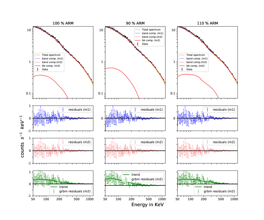
| Model | Parameter | 100% ARM | 90% ARM | 110% ARM | |||
| Best fit values | |||||||
| m1 | m2 | m1 | m2 | m1 | m2 | ||
| Band | alpha | -0.5 0.01 | -0.52 0.02 | -0.54 0.12 | -0.52 0.02 | -0.47 0.01 | -0.53 0.04 |
| beta | -2.27 0.04 | -2.32 0.05 | -2.27 0.04 | -2.32 0.05 | -2.28 0.04 | -2.33 0.06 | |
| 542 12 | 575 28 | 553 12.5 | 572 22 | 531 11 | 601 48 | ||
| norm/ | 42.5 0.25 | 40.3 0.9 | 44.1 0.25 | 41.0 0.8 | 40.9 0.24 | 38.2 1.35 | |
| Black | – | 67.2 15.1 | – | 52.3 7.8 | – | 94.3 13.7 | |
| Body | norm | – | 1.3 0.7 | – | 1.43 0.4 | – | 2.5 1.6 |
| (DOF) | 560 (550) | 554 (548) | 566 (550) | 542 (548) | 560 (550) | 555 (548) | |
It can be seen from Table 4 (and Figure 6) that when 100% ARM is considered, we accurately recover the incident band parameters. Further if we try to include a bb component in this case, the value decreases only marginally by 6 for 2 additional Degrees of Freedom (DOF) from model m1 to model m2. On the other hand, when we use an underestimated ARM, the best-fit (with m1) band component appears softer ( decreases) as compared to the incident pure band spectrum. Addition of a black body component (using model m2) improves the quality of the fit with prominent blackbody component being “detected” in data, though the source model is a pure band spectrum (Figure 6, middle column). In this case, the value decreases by 24 for two additional DOFs. This additive model component is shown by the solid red line in the top panel, and also by the green “grbm residuals (m2)” sub-plot. The error estimate on the blackbody norm indicates a statistically significant fit — arising out of ignored / unknown systematic errors in the ARM. Lastly, when we use overestimated ARM, the best-fit (with m1) band component appears harder ( increases) as compared to the injected source spectrum. If we directly compared this with the source spectrum, we would have seen negative residuals (not shown here) as the ARM used in fitting over-predicts the observed spectrum. Adding a blackbody component to this should imply that we are trying to fit a negative one. Even then, if we try to force-fit such a model to the data, we get a fit with the band component becoming much softer and unrealistic realizations for the blackbody parameters are obtained (evident from the unusually large kT value and large error in the norm of the balckbody in Table 4).
3.3.2 Band and blackbody spectral model:
We now consider a case where the GRB intrinsically has a blackbody component. We simulate a source spectrum with the same band function as before, and an additive blackbody characterised by kT=40 keV and norm=5. The temperature and relative intensity of this component are consistent with typical blackbody components detected in some GRBs.
Since the source has an intrinsic blackbody, fits with a pure band function always give poor results and we do not disucuss those. Instead, we focus our attention on modelling the spectrum with the m2 model comprising of the band spectrum and a blackbody (Figure 7, Table 5). As before, we find that if the ARM is correct, then the parameters are recovered well. However, any errors in the ARM will alter the values: for instance, if the ARM is underestimated, we find a brighter blackbody (see Table 5 and bottom row of the column at the middle of Figure 7), and conversely if the ARM used in the analysis overestimates the Earth reflection component, the inferred blackbody is fainter than the real value (shown by the plot at bottom-right of Figure 7). The best fit values for the model parameters are shown in Table 5. It can be seen from Table 5 that the best-fit values of the band spectrum are apparently the same in all the cases, with the error in ARM reflected mostly in the bb component (can be seen from the norm of the blackbody component).
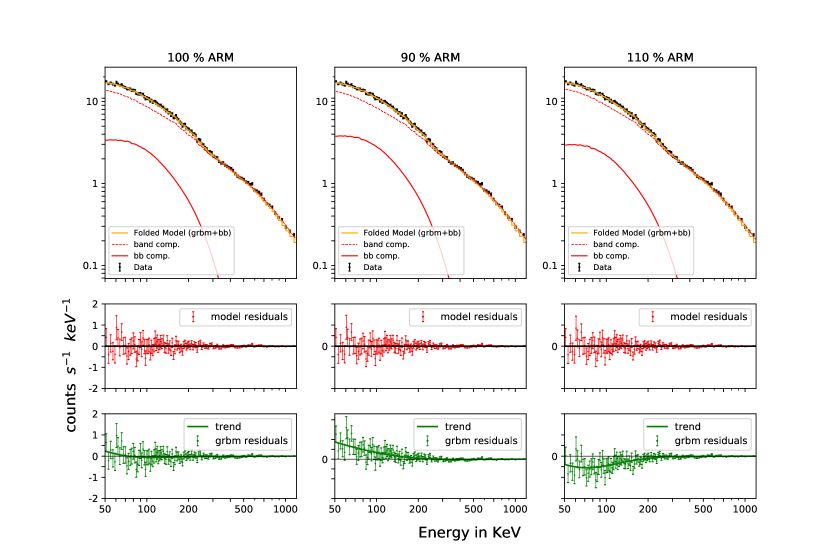
| Model | Parameter | 100% ARM | 90% ARM | 110% ARM | |
| Incident | Best fit values | ||||
| Band | alpha | -0.5 | -0.54 0.04 | -0.55 0.04 | -0.54 0.04 |
| beta | -2.25 | -2.26 0.04 | -2.26 0.05 | -2.26 0.04 | |
| 533 | 562 23 | 567 24 | 557 23 | ||
| norm/ | 42.7 | 43.4 1.1 | 43.6 1.0 | 43.3 1.0 | |
| Black Body | 40 | 40.8 1.5 | 40.2 1.3 | 41.4 1.8 | |
| norm | 5 | 4.7 0.4 | 5.31 0.37 | 4.08 0.37 | |
| (DOF) | – | 528 (548) | 530 (548) | 528 (548) | |
4 Conclusion and future work
In this study, we have presented some of our simulation outcomes helpful in better understanding the nature of the Earth’s atmospheric reflection of X-ray/–ray photons from transient space objects and how can it affect the observation. We are in the process of developing a comprehensive and open-source simulation framework for estimating the atmospheric scattered component to be used in the construction of a publicly available database on Atmospheric Response Matrix (ARM). This particular study concentrates on contemplating the significance of proper evaluation of the atmospheric reflection component in terms of its effect on prompt GRB spectral analysis. In some upcoming studies we intend to perform simulations to find out the influence of Earth’s atmospheric scattering on the determination of polarization of high energy photons from such sources.
We find that the Earth’s atmosphere is quite effective at scattering incident X-rays and –rays, creating an overall reflected spectrum that is usually strong in the 30–300 keV region. The GRB fireball model (Paczynski, 1986; Goodman, 1986; Lundman ., 2012) predicts thermal components in GRB spectra. Such components have been identified in a multitude of GRBs (for instance Ryde, 2005; Guiriec ., 2011, 2013; Iyyani ., 2013, 2015; Axelsson ., 2012; Burgess ., 2014; Nappo, F. ., 2017), and their temperatures are similar to the ones obtained in our fits above. The simplified example in §3.2 demonstrates how Earth’s reflection can mimic such a thermal component. While this component is typically modelled in analysis, §3.3 shows how even small systematic errors in the estimation of atmospheric reflection can alter our interpretations of GRB data.
The problem may be further exacerbated when accounting for the direction-dependent sensitivity of the detector instrument. For instance, the effective area of AstroSat-CZTI varies by more than two orders of magnitude over the entire sky (Mate ., 2021). If the GRB were to be incident from a low-sensitivity direction while the scattered radiation arrives from a high-sensitivity direction for the satellite, the scattered component can be an order of magnitude larger than the incident component — further magnifying the effect of any uncertainties in the scattering model.
For typical observations for which one needs smaller contribution of thermal (blackbody) flux to account for the hump in the intermediate range of prompt GRB spectra, extra care should be taken to exclude any contribution from atmospheric scattering. For example, for GRB110721A (Axelsson ., 2012; Iyyani ., 2013), blackbody is found to contribute maximum of 10% of total flux, for GRB1000724B (Guiriec ., 2011) this is found to be 4%. In these cases a slight over/under estimation of the scattering contribution may impose considerable artefacts in the analysis leading to wrong estimation of the thermal component.
This underscores the need for having robust ARM calculations that can be used in any spectral analysis. Likewise, such calculations are also needed for localisation and polarisation analyses. The calculation of the reflected spectrum from the Earth involves several complexities like creating an accurate description of the atmosphere, accounting for all physical effects, and generating a large number of incident photons to get good statistics. Approximations have to be made at each stage to make the problem tractable, and each approximation may introduce systematic errors in the final answer, which can have significant impacts on the scientific outcomes.
It is not feasible for each mission to dedicate significant resources and undertake simulations to calculate the ARM, nor should it be necessary. Instead, it is important that a few groups independently develop response matrices, and compare their results to quantify accuracy and reliability of the answers. Further, end users should be made aware of these limitations, and inclusion of appropriate systematic errors in analysis may be recommended.
Going further, there are several improvements we intend to undertake. Firstly, there is a direct trade-off between using a large detector for collecting sufficient number of photons, and the resultant large differences in the scattering angles of photons that are incident on opposite ends of the detector. We will explore more simulation geometries, including multiple-detector scenarios, that will allow us to more effectively utilise all data generated in a simulation.
Second, the current simulations were carried out over a relatively coarse energy grid, at a certain incidence angle, with a modest number of photons. We plan to undertake convergence studies to determine the step sizes required in energies and angles to ensure reliable simulation results. We will also quantify the relationship between the number of photons in each monochromatic beam and the statistical uncertainty in the final reflected spectrum. Once these requirements are clearly defined, we will undertake simulations to create a database that can be re-used for all further calculations.
The final source codes and outputs of our simulations will be made available publicly for scrutiny and reuse, in a format that may be easily repurposed for other missions.
Acknowledgements
CZT–Imager is built by a consortium of Institutes across India. The Tata Institute of Fundamental Research, Mumbai, led the effort with instrument design and development. Vikram Sarabhai Space Centre, Thiruvananthapuram provided the electronic design, assembly and testing. ISRO Satellite Centre (ISAC), Bengaluru provided the mechanical design, quality consultation and project management. The Inter University Centre for Astronomy and Astrophysics (IUCAA), Pune did the Coded Mask design, instrument calibration, and Payload Operation Centre. Space Application Centre (SAC) at Ahmedabad provided the analysis software. Physical Research Laboratory (PRL) Ahmedabad, provided the polarisation detection algorithm and ground calibration. A vast number of industries participated in the fabrication and the University sector pitched in by participating in the test and evaluation of the payload.
The Indian Space Research Organisation funded, managed and facilitated the project.
Sourav Palit wants to thank Indian Institute of Technology Bombay (IITB) for providing the scholarship and necessary resources to be able to perform this study.
References
- Agostinelli . (2003) Agostinelli, S., . 2003, Nucl. Instrum. Meth. A, 506, 250
- Axelsson . (2012) Axelsson, M., Baldini, L., Barbiellini, G., . 2012, The Astrophysical Journal, 757, L31
- Band . (1993) Band, D., Matteson, J., Ford, L., . 1993, ApJ, 413, 281
- Bhalerao . (2017a) Bhalerao, V., Kasliwal, M., Bhattacharya, D., . 2017a, Astrophysical Journal, 845, arXiv:1706.00024
- Bhalerao . (2017b) Bhalerao, V., Bhattacharya, D., Vibhute, A., . 2017b, Journal of Astrophysics and Astronomy, 38, 31
- Bisnovatyi-Kogan & Blinnikov (1977) Bisnovatyi-Kogan, G. S., & Blinnikov, S. I. 1977, A&A, 59, 111
- Burgess . (2014) Burgess, J. M., Preece, R. D., Connaughton, V., . 2014, The Astrophysical Journal, 784, 17
- Chattopadhyay . (2018) Chattopadhyay, T., Falcone, A. D., Burrows, D. N., Fox, D. B., & Palmer, D. 2018, arXiv:1807.03333
- Chattopadhyay . (2019) Chattopadhyay, T., Vadawale, S. V., Aarthy, E., . 2019, ApJ, 884, 123
- Churazov . (2008) Churazov, E., Sazonov, S., Sunyaev, R., & Revnivtsev, M. 2008, Monthly Notices of the Royal Astronomical Society, 385, 719
- Connaughton . (2015) Connaughton, V., Briggs, M. S., Goldstein, A., . 2015, The Astrophysical Journal Supplement Series, 216, 32
- Cordier . (2015) Cordier, B., Wei, J., Atteia, J. L., . 2015, arXiv e-prints, arXiv:1512.03323
- Cullen (1995) Cullen, D. E. 1995, Nuclear Instruments and Methods in Physics Research Section B: Beam Interactions with Materials and Atoms, 101, 499
- Fuschino . (2019) Fuschino, F., Campana, R., Labanti, C., . 2019, Nuclear Instruments and Methods in Physics Research A, 936, 199
- Goodman (1986) Goodman, J. 1986, ApJ, 308, L47
- Guiriec . (2011) Guiriec, S., Connaughton, V., Briggs, M. S., . 2011, The Astrophysical Journal, 727, L33
- Guiriec . (2013) Guiriec, S., Daigne, F., Hascoët, R., . 2013, The Astrophysical Journal, 770, 32
- Hedin (1991) Hedin, A. E. 1991, Journal of Geophysical Research: Space Physics, 96, 1159
- Hoover . (2005) Hoover, A. S., Kippen, R. M., Meegan, C. A., . 2005, Nuovo Cimento C Geophysics Space Physics C, 28, 797
- Hulsman . (2020) Hulsman, J., . 2020, Proc. SPIE Int. Soc. Opt. Eng., 11444, 1
- Iyyani . (2013) Iyyani, S., Ryde, F., Axelsson, M., . 2013, Monthly Notices of the Royal Astronomical Society, 433, 2739
- Iyyani . (2015) Iyyani, S., Ryde, F., Ahlgren, B., . 2015, Monthly Notices of the Royal Astronomical Society, 450, 1651
- Kippen . (2007) Kippen, R. M., Hoover, A. S., Wallace, M. S., . 2007, AIP Conference Proceedings, 921, 590
- Klein & Nishina (1929) Klein, O., & Nishina, T. 1929, Zeitschrift fur Physik, 52, 853
- Lundman . (2012) Lundman, C., Pe’er, A., & Ryde, F. 2012, Monthly Notices of the Royal Astronomical Society, 428, 2430
- Mate . (2021) Mate, S., Chattopadhyay, T., Bhalerao, V., . 2021, Journal of Astrophysics and Astronomy accepted for publication
- McConnell . (2017) McConnell, M. L., Baring, M. G., Bloser, P. F., . 2017, in AAS/High Energy Astrophysics Division, Vol. 16, AAS/High Energy Astrophysics Division #16, 103.20
- Meegan . (2009) Meegan, C., Lichti, G., Bhat, P. N., . 2009, The Astrophysical Journal, 702, 791
- Nappo, F. . (2017) Nappo, F., Pescalli, A., Oganesyan, G., . 2017, A&A, 598, A23
- Paczynski (1986) Paczynski, B. 1986, ApJ, 308, L43
- Palit . (2013) Palit, S., Basak, T., Mondal, S. K., Pal, S., & Chakrabarti, S. K. 2013, Atmospheric Chemistry and Physics, 13, 9159
- Palit . (2018) Palit, S., Raulin, J., & Szpigel, S. 2018, Journal of Geophysical Research: Space Physics, 123, 10,224
- Pendleton . (1999) Pendleton, G. N., Briggs, M. S., Kippen, R. M., . 1999, ApJ, 512, 362
- Racusin . (2017) Racusin, J., Perkins, J. S., Briggs, M. S., . 2017, arXiv e-prints, arXiv:1708.09292
- Rao . (2017) Rao, A., Bhattacharya, D., Bhalerao, V., Vadawale, S., & Sreekumar, S. 2017, Current Science, 113, doi:10.18520/cs/v113/i04/595-598
- Ryde (2005) Ryde, F. 2005, The Astrophysical Journal, 625, L95–L98
- Sazonov . (2007) Sazonov, S., Churazov, E., Sunyaev, R., & Revnivtsev, M. 2007, Monthly Notices of the Royal Astronomical Society, 377, 1726
- Sempau . (2003) Sempau, J., Fernández-Varea, J., Acosta, E., & Salvat, F. 2003, Nuclear Instruments and Methods in Physics Research Section B: Beam Interactions with Materials and Atoms, 207, 107
- Sharma . (2020) Sharma, Y., Marathe, A., Bhalerao, V., . 2020, arXiv e-prints, arXiv:2011.07067
- Singh . (2014) Singh, K. P., Tandon, S. N., Agrawal, P. C., . 2014, in Proc. SPIE, Vol. 9144, Space Telescopes and Instrumentation 2014: Ultraviolet to Gamma Ray, 91441S
- Wanderman & Piran (2015) Wanderman, D., & Piran, T. 2015, MNRAS, 448, 3026
- Werner . (2018) Werner, N., Pál, A., Ohno, M., . 2018, in Space Telescopes and Instrumentation 2018: Ultraviolet to Gamma Ray, ed. J.-W. A. den Herder, K. Nakazawa, & S. Nikzad (SPIE), 96
- White . (1988) White, T. R., Lightman, A. P., & Zdziarski, A. A. 1988, ApJ, 331, 939
- Willis . (2005) Willis, D. R., Barlow, E. J., Bird, A. J., . 2005, A&A, 439, 245
- Zhang . (2019) Zhang, D., Li, X., Xiong, S., . 2019, Nuclear Instruments and Methods in Physics Research, Section A: Accelerators, Spectrometers, Detectors and Associated Equipment, 921, 8