Rhombic Tilings and Primordia Fronts of Phyllotaxis
Abstract
We introduce and study properties of phyllotactic and rhombic tilings on the cylinder. These are discrete sets of points that generalize cylindrical lattices. Rhombic tilings appear as periodic orbits of a discrete dynamical system that models plant pattern formation by stacking disks of equal radius on the cylinder. This system has the advantage of allowing several disks at the same level, and thus multi-jugate configurations. We provide partial results toward proving that the attractor for is entirely composed of rhombic tilings and is a strongly normally attracting branched manifold and conjecture that this attractor persists topologically in nearby systems. A key tool in understanding the geometry of tilings and the dynamics of is the concept of primordia front, which is a closed ring of tangent disks around the cylinder. We show how fronts determine the dynamics, including transitions of parastichy numbers, and might explain the Fibonacci number of petals often encountered in compositae.
1 Introduction
Phyllotaxis is the study of arrangements of plant organs. These originate at the growing tip (apex meristem) of a plant as protuberances of cells, called primordia. The geometric classification of phyllotactic patterns has often been reduced to that of cylindrical lattices, where the helices joining nearest primordia - called parastichies - form two families winding in opposite directions. Counting parastichies in each family gives rise to the pair of parastichy numbers that are used to classify phyllotactic patterns. The striking phenomenon central to phyllotaxis is the predominance of pairs of successive Fibonacci numbers as parastichy numbers.
However, Fibonacci patterns and transitions among these are not the only ones observed in nature. A very common transition can be seen on stems of sunflowers, for instance: after a few pairs of aligned leaves alternating at a angle leaves suddenly grow in spirals yielding Fibonacci numbers. In terms of parastichy numbers classification, the pattern with parastichy numbers , (decussate), transitions to . This transition is usually absent from the analysis of dynamical models of phyllotaxis, even when they can reproduce it. More generally, transitions to and from multijugate phyllotaxis, where parastichy numbers have a common divisor , and where organs appear at the same level (whorl), is not often discussed ([douadycouder], Parts II & III being a notable exception). Part of the difficulty lied in the absence, in the literature, of a continuum of patterns encompassing lattices of all jugacies, and of more local geometric tools to follow the transitions as they unfold one primordium at a time.
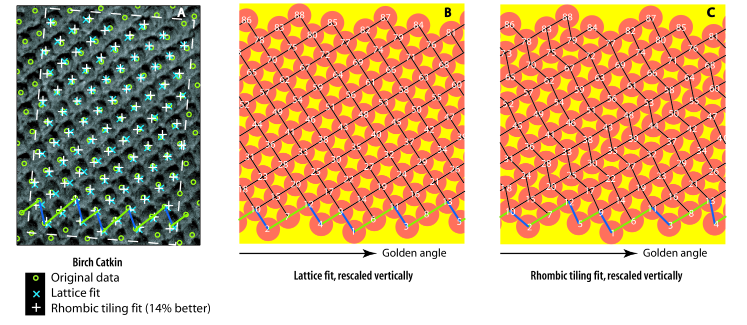
We introduce the geometric concept of phyllotactic and rhombic tilings, which do encompass lattices of all jugacies, as well as patterns hitherto considered as transient. These tilings can be seen as deformations of cylindrical lattices. In contrast with lattices, they can account for the marked undulations of parastichies often observed in nature (Fig. 1).
We also reintroduce van Iterson’s century old concept of “zickzacklinie” [vaniterson], that we call here primordia fronts (Fig. 1). These zig-zaging fronts and their parastichy numbers offer a practical and theoretical tool to understand not only the steady state tilings but also transitions from one to another, in a way that may be less confusing than the divergence angles often used in experiments (see e.g. Section 2.2). The concept of primordia front might also offer an explanation as to the statistical predominance of Fibonacci numbers of ray petals in many asteracea ([battjes]): the number of primordia in a front is the sum of its Fibonacci (likely) parastichy numbers, hence itself a (likely) Fibonacci number.
We root the concepts of tilings and fronts within a simple discrete dynamical model that more or less explicitly exists since the 19th century ([weisse], [vaniterson], [williams], [douady]). This system, that we call the Snow map after [douadycouder] and denote by , represents primordia formation as the stacking of disks on a cylinder, according to the simple rules: the new disk appears at the lowest level above the older ones, without overlap. As we fix the circumference of the cylinder, the diameter of the of the primordia is the fundamental parameter of this model.
Theorem LABEL:thm:attractor, brings together the geometry and dynamics of this paper, by showing that, for each parastichy number pair and for in an appropriate range, there exists a manifold of rhombic tilings, each of which is a periodic orbit of period for . This manifold is of dimension , and contains the -lattice of the fixed point bifurcation diagram for that (see Section LABEL:subsec:fp.po). We also show that this manifold is a local attractor for , and that the attraction occurs in finite time.
We conjecture that the entire set of dynamically sustainable rhombic tilings forms a normally attracting set. This should imply the persistence of an invariant set with comparable topology in nearby models ([fenichel]) and would confer the Snow model and rhombic tilings some universality in phyllotaxis.
Although we do not study phyllotactic transitions in great detail here (see Sections 2.2 and LABEL:subsec:frontdyn), we hope that this paper will serve as foundation for further research in that direction. Later work will explore the topological structure of the set of dynamically sustainable tilings, and of the dynamical transitions it allows, as well as generalizations of these tilings to other geometries. Experimental applications of some of the concepts discussed here, such as using fronts derived from plant data as initial conditions for growth modeling using a similar model, appeared in [jpgr].
Recent experimental and modeling work points to the active transport of the hormone auxin [auxinbern], [auxintraas],[auxinmjolsness], [auxinprunsi] as the underlying mechanism of primordia formation, although some authors still advocate for a buckling explanation [shipman]. Although the type of models based on auxin transport should eventually prove invaluable in testing the validity of proposed biological mechanisms, to date they can’t easily and stably reproduce Fibonacci phyllotaxis, and neither could they form the proper context for a geometrical explanation of its prominence. Our approach is grounded in the tradition of dynamical/geometric models ([weisse],[vaniterson], [williams], [adler], [douadycouder], [douady], [leelevitov], [kunzthesis], [jns]), often based on the botanical observations of Hofmeister [hofmeister] and Snow & Snow [snow]. The model we study is also compatible with the general assumptions of [auxinbern] and [shipman]. Our goal is to distill to their simplest and most rigorous form the geometric mechanisms that could be at play in Phyllotactic pattern formation. The concepts we develop are general enough that they may adapt to other situations, such as the assembly of the HIV-1 CA protein [HIVnature].
To motivate this otherwise rather theoretical paper, we start in Section 2 by reporting on some numerical experiments, showing how phenomena encountered by iterating on a computer naturally lead to rhombic tilings and primordia fronts. We then review the classical geometry of the cylindrical lattices and of their parastichies (Section 3). In Section 4.1, we establish the notion, for general configurations of primordia, of chains and fronts of primordia as sets of tangent primordia encircling the meristem. The parastichy numbers of chains and fronts are just the number of up and down segments as one travels around the chain. The definition of phyllotactic and rhombic tiling as cyclic sums of up and down vectors follows in Section 4.2, followed by the analysis of their periodicity and properties of parastichies. In Section LABEL:subsec:parastnum, we show the equality of parastichy numbers of a tiling and of any of its fronts - thus validating the usage of the front parastichy numbers.
We then give a rigorous definition of the Snow map , followed by a study of its domain of differentiability (Section LABEL:sec:snow).
Section LABEL:sec:dyngeom brings the dynamics of and the geometry of fronts and tilings together. In Section LABEL:subsec:frontdyn, we show that the top primordia front of a configuration determines its dynamical future, and that changes in parastichy numbers can be simply read from the number of sides of the polygonal tile between a new primordium and the top front. We show that the fixed points of the map induced on the shape space of configurations are the same rhombic cylindrical lattices as in the Hofmeister map of [jns] and conjecture that periodic orbits all form rhombic tilings (Section LABEL:subsec:fp.po). In Section LABEL:subsec:attractor, we prove Theorem LABEL:thm:attractor on the existence of attracting sets of rhombic tilings mentioned above. Returning to experimental results, Section LABEL:subsec:rp2 shows numerically how tilings whose parastichy numbers sum up to 4 coexist in the shape space of chains of four primordia. We show that the latter set, for the chosen parameter, has the topology of the projective plane.
2 Numerical Explorations
Before formally studying the concepts of rhombic tilings, primordia front, and their relation to the dynamics of the Snow map , we present some numerical observations that motivated our theoretical inquiry.
2.1 Asymptotic Behavior of
In our numerical simulations, we consistently observed that, under iterations of , all configurations converge to of “fat rhombic tilings”: lattice-like sets of points of the cylinder that are vertices of tilings with rhombic tiles that are not too thin (See Section 4.2). The tilings have, like the classical lattices of phyllotaxis, parastichies: strings of tangent primordia winding up and down the cylinder in somewhat irregular helices. And as with lattices, these parastichies come in two families winding in opposite directions (Fig 2).
Interestingly, we observed two distinct types of convergence to rhombic tilings: a finite time convergence and an asymptotic (infinite time) convergence. In our experiments, asymptotic convergence always involves at least one pair of pentagonal and triangular tiles, repeating along a parastichy (Fig. 2). One can see from the figure (see Proposition LABEL:prop:frontperiod for a proof) that when an orbit goes through segments of a given rhombic tiling of parastichy numbers its shape repeats periodically, with period . Hence, orbits that we have observed are either periodic (in the shape space), preperiodic or asymptotically periodic (with triangle and pentagon pairs). Moreover we observed large continua of tiling segments that are periodic orbits. In Theorem LABEL:thm:attractor, we prove the existence of such continua and of the preperiodicity of all orbits near steady state lattices. We will leave the analysis of the asymptotic convergence to a later work.
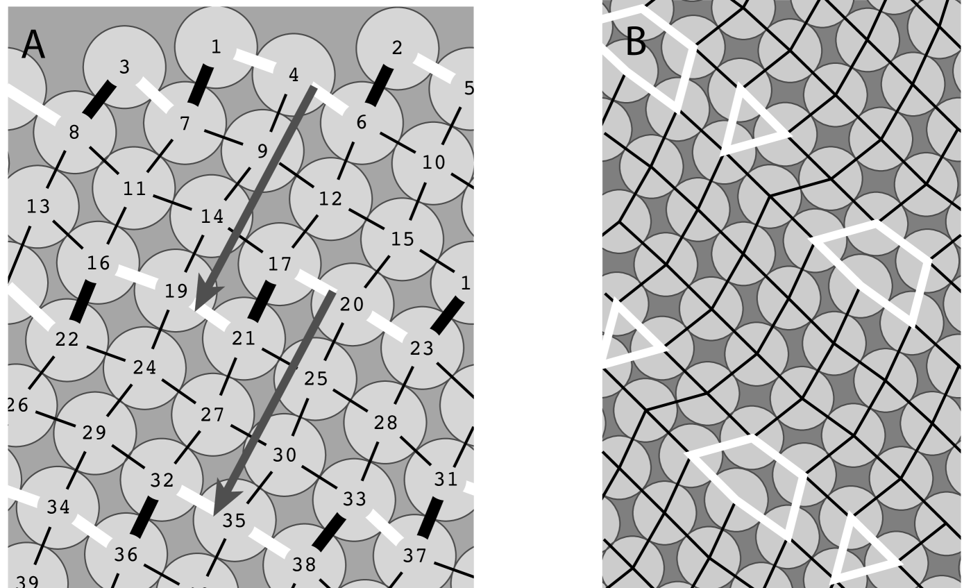
It is intuitively clear that, at a given time step. of the iteration, the top connected layer of primordia holds the key to the dynamics and the geometry of the orbits. We call such a layer a primordia front (Section 4.1). The number of “up” and “down” vectors forming the zigzagging curve as one travels from left to right on a front corresponds to parastichy numbers in the case of lattices and tilings (Proposition LABEL:prop:parastnum). We call them front parastichy numbers (Section 4.1). We contend that counting front parastichy numbers at each step of the iteration - which can be programmed in either simulations or data analysis - may be less misleading than the divergence angles commonly used in this type of experiment (See Figures 1 and 3 and the next section).
2.2 The Fibonacci Path
The litmus test for a model of phyllotaxis is its ability to reproduce aspects of the bifurcation diagram - or fixed point set - of Section LABEL:subsec:fp.po, and especially of its Fibonacci branch.
This diagram is formed by the generators (see Section 3) of the “good” lattices of phyllotaxis, that are steady states of the given model (in this case presented, of both and the Hofmeister map of [jns]). Each (dark) curve segment of the diagram corresponds to lattices with a given pair of parastichy numbers whose shapes are fixed under . The coordinate of a generator corresponds to the so-called divergence angle between two consecutive points in the vertical ordering of the lattice. It also corresponds to the difference of coordinate of the new primordium and the next in an iteration process. The divergence angle, and its connection to parastichy numbers in lattices, has been widely used to explain and detect in models the Fibonacci phenomenon [douadycouder]. The Fibonacci branch of the bifurcation diagram is the largest in the diagram, and starts at lattices of parastichy numbers (1,1), corresponding to the beginning of the growth of most monocotyledonous plants. In our work on the Hofmeister map [jns], we showed that the steady state lattices are attractors, accounting for the fact that once near the Fibonacci branch, a configuration remains near it as the parameter (in that case the internodal distance) was decreased.
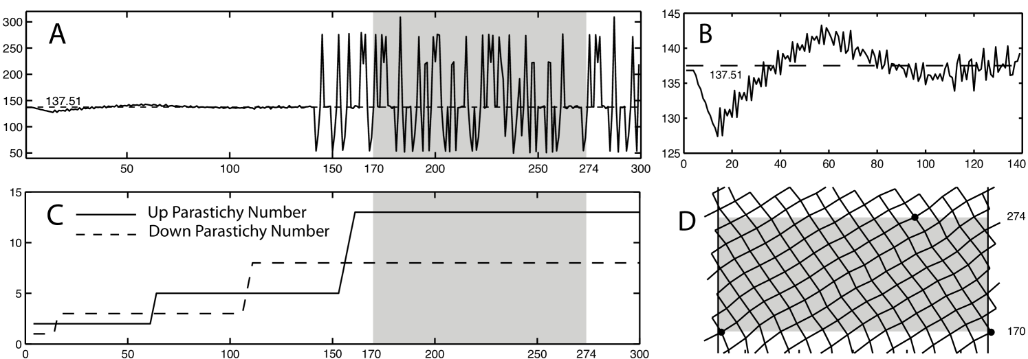
We were originally pessimistic about yielding Fibonacci transitions as the parameter varies. Indeed, we had observed numerically that a steady state lattice for is part of an attracting manifold of periodic orbits and the eigenvalues of the differential are either 0 or on the unit circle (A consequence of Theorem LABEL:thm:attractor). Hence the steady states for can at best be neutrally stable. However, our experiments (Fig. 3 (A & B)) show that, as we lower the diameter of the primordia while iterating , the Fibonacci phenomenon, as measured by front parastichy numbers, is in fact much more robust in our model than the divergence angle measurements indicates: while the divergence angle can vary wildly even in an orbit close to a lattice, the parastichy numbers stay constant. Orbits do not have to stay too close to lattices to follow the Fibonacci route: It is sufficient that they stay in a neighborhood the substantially larger and attracting set of rhombic tilings. This flexibility allows for much faster transitions than previously thought, in a time scale observed in plants, as we will show in future work. Last but not least, the strong attraction of orbits to the set of rhombic tilings should make this set persist topologically in nearby systems.
3 Classical Geometry of Phyllotaxis
3.1 Underlying Geometry
In this paper, we concentrate on cylindrical phyllotaxis. We normalize the cylinder to have circumference 1. Mathematically, is the cartesian product of the unit circle with the reals. Note that fixing the circumference of the cylinder does not mean that we preclude lateral plant growth in our modeling. We make this convenient normalization choice without loss of generality since, in the patterns we study, the important parameters (such as the ratio of the size of primordia relative to the diameter of the meristem) are independent of scale. Both botanists and mathematicians often unroll cylindrical patterns on the plane , which can also be seen as the complex plane . This is the covering space of the cylinder (see Section 3.2). We will use the same notation for points and vectors in and . By a configuration, we mean a finite set of points in ordered by height. These points represent centers of primordia along the stem.
3.2 Covering Space Notions and Notation
We often describe objects in the cylinder via their covers and lifts in the plane. The intuitive notion of cover of a set, in the case of the cylinder is simple: mark each point of the set with ink, and use the cylinder as a rolling press. As you roll the cylinder indefinitely on the plane, the points printed form the cover of the original set. Each piece of the cylindrical pattern is repeated at integer intervals along the -direction. The cover of a helix, for example, is a collection of parallel lines. The lift of a helix at a point is the choice of one of these lines.
Here is a more rigorous description of these classical concepts [munkres] and notation that we will be using. The natural projection which maps a point to is a covering map and the plane is a covering space of the cylinder . This means that is surjective, and that around any point of , there exists an open neighborhood such that (the inverse image of ) is a disjoint union of open sets of the plane each homeomorphic to . One says that is a local homeomorphism and that is evenly covered. In the case of the cylinder, is also a local isometry, for the metric induced by on the cylinder. A subset of is a fundamental domain if is a bijection. Any region of of the form is a fundamental domain.
The cover of a subset of is the inverse image of . A set of the plane is a cover of its projection if and only if The “tilde” notation as above is often used to denote covering spaces. In this paper, we also use the underline notation to denote the projection of a set in the plane to the cylinder: .
As with all covering maps, has the lifting property: if is a path in and is a point “lying over” (i.e. ), then there exists a unique path lying over (i.e. ) and with . The curve is called the lift of at .The lift of a path is only a connected part of its cover: for instance the lift at of the line of equation of the cylinder is the line in the plane, whereas its cover is the union of all the lines
3.3 Cylindrical Lattices, Helical Lattices, Multijugate Configurations
A cylindrical lattice is a set of points in whose cover is a lattice of :
where are independent generating vectors. Note that a discrete subgroup of isomorphic to . Since is a cover, it must be invariant under translation by . Changing bases if necessary, one can assume that for some positive integer , called the jugacy of the lattice.
If , we say that is monojugate or that it is a helical lattice. In this case and has the unique generator . If , is called a multijugate configuration or specifically a jugate configuration (or -jugate lattice). A cylindrical lattice is a discrete subgroup of isomorphic to (simply in the case of a helical lattice). In a -jugate lattice, each point is part of a set of points, called a whorl, evenly spread around a horizontal circumference of .
Parastichies of a helical lattice are helixes joining each point of to its nearest neighbors. We now make this more precise. In general, there are two points of nearest to in the positive half plane. Say and nearest to 0, where . Also assume that makes a larger angle with the horizontal than , so in particular and are not colinear. The line through 0 and lifts a helix in that contains all the points . The set of these points is called a parastichy, and the helix connecting them a connected parastichy. There are helixes, also called parastichies, parallel to this one. Each goes through a set of points , for a fixed . To prove this, one shows that when , one obtains another lift of the original parastichy, using
| (1) |
This is a consequence of being closest to 0 ([jns], Proposition 4.2) and it implies that and are co-prime (). Thus there are parastichies and they correspond to a cosets of the subgroup of . Likewise, there are parallel parastichies joining the second closest neighbors.
If is a -jugate lattice, we can trace parastichies through nearest neighbors in a similar fashion. This time the parastichy numbers and must have the common divisor . An intuitive way to see this is that, rescaling the cover of by , one obtains the cover of a helical lattice, call it . Build the parastichies through nearest neighbors for as before. Then rescale back by - the rescaled parastichies are parastichies of . Since you need copies of the rescaled to go around the cylinder, you need rescaled copies of each parastichy of , crossing the -axis at intervals of , to get all the parastichies of .
Thus, all cylindrical lattices can be classified by their parastichy numbers where is the number of primordia in a whorl. Helical lattices are the special case where . Whorled configurations, where primordia in a new whorl are placed midway between those of the previous whorl, is another notable case, which corresponds to .
3.4 Limitations of Cylindrical Lattices in Phyllotaxis.
In Section 2.2, we presented a numerical simulation showing Fibonacci transitions along orbits of when the parameter is decreased. We argued briefly that the dynamical transitions observed mirrored the continuous geometric deformation of helical lattices along the main Fibonacci branch of the bifurcation diagram. The existence of the (connected) Fibonacci branch has been the basis of many explanations of the phenomenon since the century111This neat geometric fact has often been a source of confusion between the global deformation of a pattern and its transitions via a dynamical process with varying parameter. ([weisse], [vaniterson]). Unfortunately, this kind of argument, made rigorous for the Hofmeister model in [jns], cannot work for transitions involving a change of jugacy in the pattern. One of these transitions, from (decussate) to (Fibonacci spiral) is the norm in the vast majority of dycotyledonous plants such as the sunflower, where after a few whorls of two leaves at angle, symmetry is broken and a spiral pattern emerges. This transition cannot be attributed to the proximity of iterated patterns to a continuous path within the set of lattices between lattices of parastichy numbers and . Indeed, no such continuous path exists, since it would have to involve the continuous deformation of the vector into within the discrete set of rational vectors of the form , which is clearly absurd.
Even in a Fibonacci transition, the global geometric deformation of lattices (orthostichies becoming parastichies when decreases) does not translate easily into a dynamical understanding of the transitional region. In short, we need more flexible and local geometrical tools to better describe dynamical transitions.
4 New Geometry for Phyllotaxis
In this section, we introduce primordia fronts and phyllotactic tilings. They address the limitations noted in the previous paragraph. Fronts are local in nature and are well defined in the setting of general configurations of points of the cylinder. We will show that fronts are key in understanding transitions. Phyllotactic tilings and more specifically rhombic tilings allow many more deformations than cylindrical lattices while still featuring parastichies. We give an algebraic definition of these tilings as a set of points obtained by cyclically adding “up” and “down” vectors. In later sections, we derive the geometric and periodicity properties of these tilings and of the tiles they bound.
4.1 Parents, Ontogenetic Graphs, Fronts, Local Parastichy Numbers
This subsection gives definitions regarding very general configurations of points of the cylinder. They can naturally be adapted to other geometries (cone or disk) as well (see [jpgr]). We consider general configurations of a number of disks of a given diameter in the cylinder. These configurations are given by their centers and they form the set , Cartesian product of copies of the cylinder. Occasionally, we need to consider countably infinite configurations as well.
The ontogenetic order for a configuration in is a choice of indices for the points which corresponds to the following order of the points coordinates:
where we choose the fundamental domain .
Often, such as with lattices, we consider finite configurations that are pieces of infinite ones. A configuration comprising all the points of an infinite configuration between some and in the ontogenetic order of is called a segment of of length .
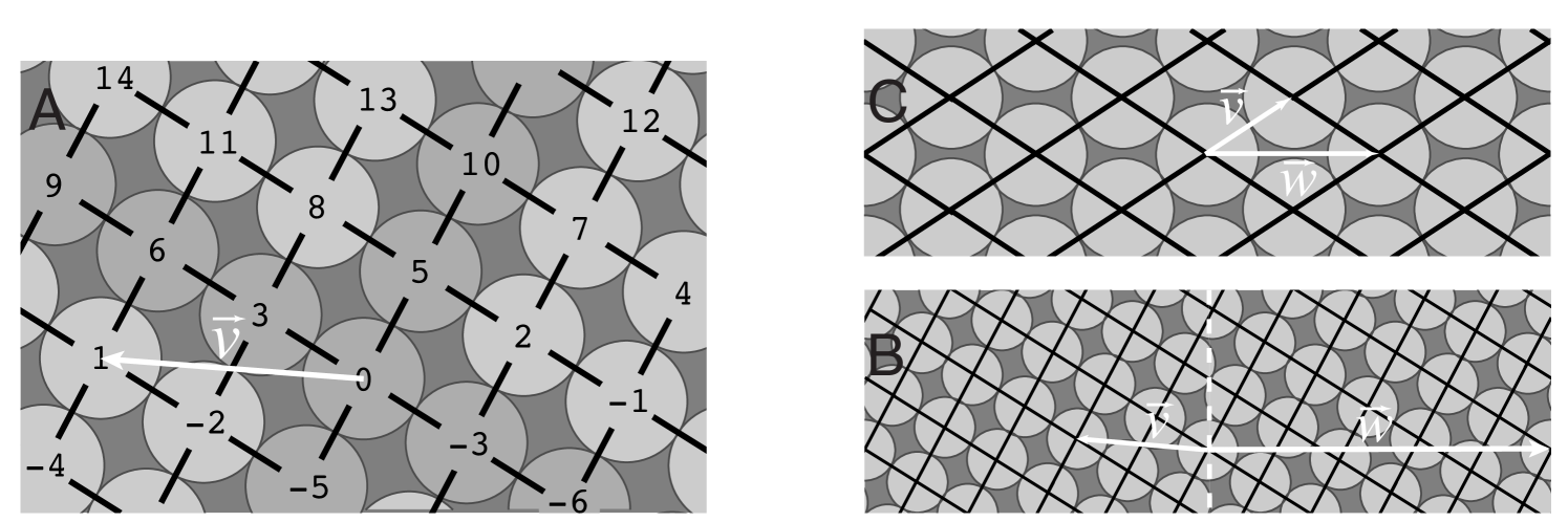
A primordium is a left (resp. right) parent of if it is tangent below and to the left (resp. right) of . More precisely, we adopt the convention that, for to be left parent of , the coordinates of the vector must satisfy and , and for to be right parent of . In the obvious fashion, is a right (resp. left) child of if is a left (resp. right) parent of .
The ontogenetic graph of a primordia configuration is the directed graph embedded in whose vertices are the centers of the primordia and where oriented edges are drawn between primordia and their parents (if they have any).
Given an ontogenetically ordered configuration of , we call parents data the information about which primordia are parents of which primordia. One way to represent this data is by a parents data matrix, whose entry is if is left parent of , if is right parent of and 0 if is not a parent of . Note that the absolute value of this matrix is just the adjacency matrix of the (directed) ontogenetic graph.
A primordia chain for a configuration is a subset of distinct points in the configuration such that:
-
•
The chain is connected by tangencies: for all , primordium is either a right parent or right child of . A chain can thus be represented by a piecewise linear curve through the centers of its primordia, which can be lifted to .
-
•
The chain is closed and does not fold over itself: the point is either a left parent or left child of and any lift at a point with of the chain is the graph of a piecewise linear function over the axis in joining to its translate .
The vector is an up vector of the chain if is a right child of .
The vector is a down vector if is a right parent of .
We call the number of up (resp.down) vectors in a chain its right (resp.left) parastichy number.
If is always parent of for and then always a child for , we call the chain a necklace.
Given a configuration ordered ontogenetically, a front at is a chain with primordia of indices greater or equal to , such that any primordium (not necessarily in the configuration) which is the child of a primordium in the chain, without overlapping any other primordium in the chain, is necessarily at a height greater or equal to that of . The parastichy numbers of a front are called front parastichy numbers.
Remark 4.1.
Most of the notions defined above are applicable to plant data by relaxing the definition of left (resp. right) parent to that of “closest primordia below to the left (resp. to the right)” with some tolerance level. In the case of configurations on the disk, “below” translates to “farther away from the meristem” (see [jpgr]). Algorithms using these notions were also used to produce Fig. 1 and [fig:divVSparast].
4.2 Phyllotactic Tilings
A Phyllotactic tiling is a set of points of that can be obtained by summing to a base point cyclically ordered sums of “up” and “down” vectors. More precisely, a tiling is determined by a base point , down vectors where each has components , and up vectors , each with components . Moreover, we ask that
| (2) |
We then define
where with:
and where
| (3) |
and we use the periodicity convention . The function is a cyclical sum of up vectors defined similarly, with the convention that . The numbers of down and up vectors are called the parastichy numbers of the tiling, a terminology justified by Proposition LABEL:prop:paras.
The phyllotactic tiling is rhombic if all the up and down vectors have same length , and we call the length of the tiling. A fat tiling is a phyllotactic tiling such that the angles between any two down and up vectors are in the interval . It is not hard to see that the ontogenetic graph of a rhombic tiling is the embedded graph in the cylinder whose vertices are the points of the tiling and the edges are the down and negative up vectors connecting them. For general phyllotactic tiling, we call this graph the graph of the tiling. We call the connected components of the complement of the graph its tiles.