Rigidity, tensegrity and reconstruction of polytopes under metric constraints

Martin Winter Mathematics Institute, University of Warwick, Coventry CV4 7AL, United Kingdom martin.h.winter@warwick.ac.uk

(Date: October 1, 2025)

Abstract.

We conjecture that a convex polytope is uniquely determined up to isometry by its edge-graph, edge lengths and the collection of distances of its vertices to some arbitrary interior point, across all dimensions and all combinatorial types. We conjecture even stronger that for two polytopes $P\subset\mathbb{R}^{d}$ and $Q\subset\mathbb{R}^{e}$ with the same edge-graph it is not possible that $Q$ has longer edges than $P$ while also having smaller vertex-point distances.

We develop techniques to attack these questions and we verify them in three relevant special cases: $P$ and $Q$ are centrally symmetric, $Q$ is a slight perturbation of $P$ , and $P$ and $Q$ are combinatorially equivalent. In the first two cases the statements stay true if we replace $Q$ by some graph embedding $q\colon V(G_{P})\to\mathbb{R}^{e}$ of the edge-graph $G_{P}$ of $P$ , which can be interpreted as local resp. universal rigidity of certain tensegrity frameworks. We also establish that a polytope is uniquely determined up to affine equivalence by its edge-graph, edge lengths and the Wachspress coordinates of an arbitrary interior point.

We close with a broad overview of related and subsequent questions.

Key words and phrases:

convex polytopes, reconstruction from the edge-graph, Wachspress coordinates, rigidity and tensegrity of frameworks

2010 Mathematics Subject Classification:

51M20, 52B11, 52C25

1. Introduction

In how far can a convex polytope be reconstructed from partial combinatorial and geometric data, such as its edge-graph, edge lengths, dihedral angles, etc., optionally up to combinatorial type, affine equivalence, or even isometry? Questions of this nature have a long history and are intimately linked to the various notions of rigidity.

In this article we address the reconstruction from the edge-graph and some “graph-compatible” distance data, such as edge lengths. It is well-understood that the edge-graph alone carries very little information about the polytope’s full combinatorics, and trying to fix this by supplementing additional metric data reveals two opposing effects at play.

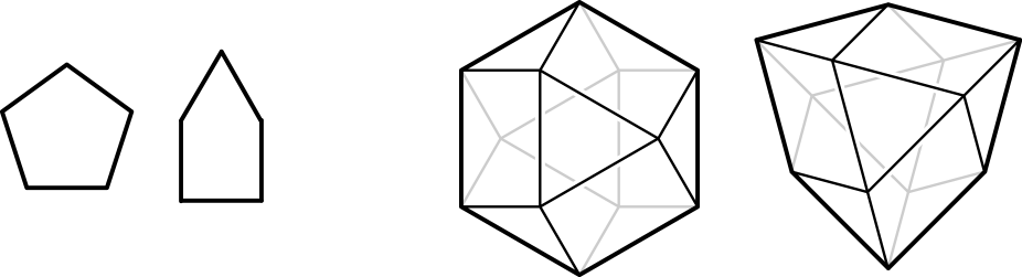
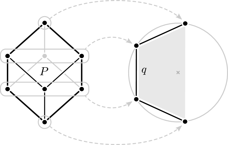
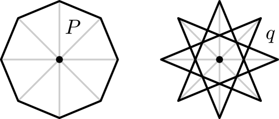
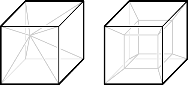
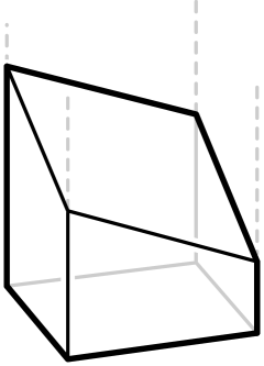
First and foremost, we need to reconstruct the full combinatorics. As a general rule of thumb, reconstruction from the edge-graph appears more tractable for polytope that have relatively few edges (such as simple polytopes as proven by Blind & Mani [2] and later by Kalai [19])¹¹1Though “few edges” is not the best way to capture this in general, see [8] or [17].. At the same time however such polytopes often have too few edges to encode sufficient metric data for reconstructing the geometry. This is most evident for polygons, but happens non-trivially in higher dimensions and with non-simple polytopes as well (see Figure˜1).

Refer to caption — Figure 1. Non-isometric realizations with the same edge lenghts.

In contrast, simplicial polytopes have many edges and it follows from Cauchy’s rigidity theorem that such are determined up to isometry from their edge lengths; if we assume knowledge of the full combinatorics. For simplicial polytopes however, the edge-graph alone is usually not enough to reconstruct the combinatorics in the first place (as evidenced by the abundance of neighborly polytopes).

This leads to the following question: how much and what kind of data do we need to supplement to the edge-graph to permit

()

unique reconstruction of the combinatorics, also for polytopes with many edges (such as simplicial polytopes), and at the same time,
()

unique reconstruction of the geometry, also for polytopes with few edges (such as simple polytopes).

Also, ideally the supplemented data fits into the structural framework provided by the edge-graph, that is, contains on the order of $\#\text{edges}+\#\text{vertices}$ datums.

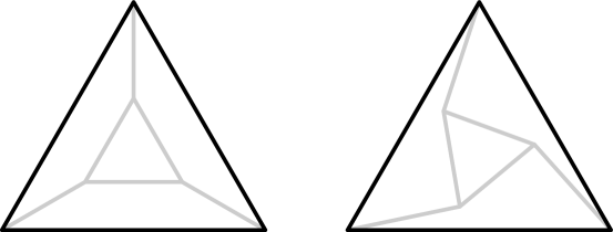
We propose the following: besides the edge-graph and edge lengths, we also fix a point in the interior of the polytope $P$ , and we record its distance to each vertex of $P$ (cf. Figure˜2). We believe that this is sufficient data to reconstruct the polytope up to isometry across all dimensions and all combinatorial types.

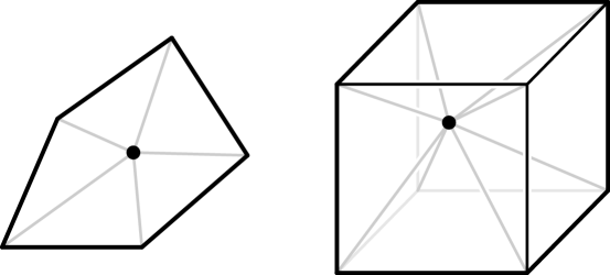
Here and in the following we can assume that the polytopes are suitably translated so that the chosen point is the origin $0\in\operatorname{int}(P)$ .

Conjecture 1.1.

Given polytopes $P\subset\mathbb{R}^{d}$ and $Q\subset\mathbb{R}^{e}$ with the origin in their respective interiors, and so that $P$ and $Q$ have isomorphic edge-graphs, corresponding edges are of the same length, and corresponding vertices have the same distance to the origin. Then $P\simeq Q$ (i.e., $P$ and $Q$ are isometric via an orthogonal transformation).

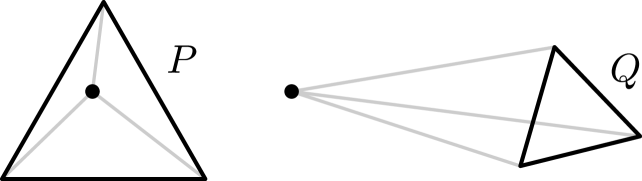
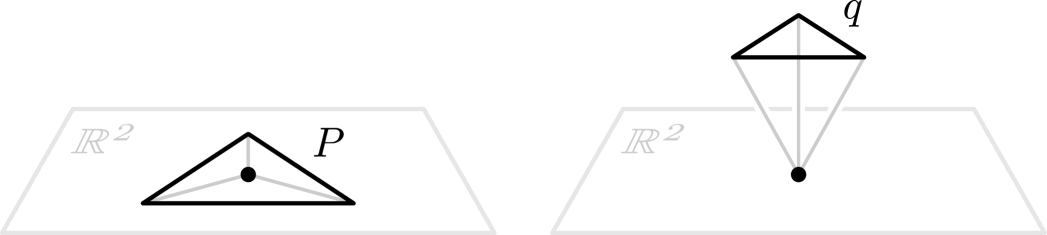
Requiring the origin to lie in the interior is necessary to prevent counterexamples such as the one shown in Figure˜3. This conjecture vastly generalizes several known reconstruction results, such as for matroid base polytopes or highly symmetric polytopes (see Section˜5.1).

We also make the following stronger conjecture:

Conjecture 1.2.

Given two polytopes $P\subset\mathbb{R}^{d}$ and $Q\subset\mathbb{R}^{e}$ with isomorphic edge-graphs, and so that

()

$0\in\operatorname{int}(Q)$ ,
()

edges in $Q$ are at most as long as their counterparts in $P$ , and
()

vertex-origin distances in $Q$ are at least as large as their counterparts in $P$ ,

then $P\simeq Q$ ( $P$ and $Q$ are isometric via an orthogonal transformations).

Intuitively, ˜1.2 states that a polytope cannot become larger (or “more expanded” as measured in vertex-origin distances) while its edges are getting shorter. It is clear that ˜1.1 is a consequence of ˜1.2, and we shall call the former the “unique reconstruction version” of the latter. Here, the necessity of the precondition $0\in\operatorname{int}(Q)$ can be seen even quicker: vertex-origin distances can be increased arbitrarily by translating the polytope just far enough away from the origin (see also Figure˜4).

In this article we develop techniques that we feel confident point us the right way towards a resolution of the conjectures. We then verify the conjectures in the following three relevant special cases:

•

$P$ and $Q$ are centrally symmetric (Theorem˜4.4),
•

$Q$ is a slight perturbation of $P$ (Theorem˜4.5),
•

$P$ and $Q$ are combinatorially equivalent (Theorem˜4.7).

The last special case clarifies, in particular, the case of 3-dimensional polytopes. Also, our eventual formulations of the first two special cases will in fact be more general, replacing $Q$ by some embedding $q\colon V(G_{P})\to\mathbb{R}^{e}$ of the edge-graph $G_{P}$ , where $q$ is no longer assumed to be the skeleton of any polytope. These results can then also be interpreted as claiming rigidity, local or universal, of certain bar-joint or tensegrity frameworks.

1.1. Notation and terminology

Throughout the article, all polytopes are convex and bounded, in particular, can be written as the convex hull of their vertices:

P=\operatorname{conv}\{p_{1},...,p_{n}\}:=\Big{\{}\smash{\sum_{i}\alpha_{i}p_{i}\mid\alpha\in\Delta_{n}}\Big{\}},

where $\Delta_{n}:=\{x\in\mathbb{R}^{n}_{\geq 0}\mid x_{1}+\cdots+x_{n}=1\}$ denotes the set of convex coefficients.

If not stated otherwise, $P\subset\mathbb{R}^{d}$ will denote a polytope in $d$ -dimensional space for $d\geq 2$ , though its affine hull $\operatorname{aff}(P)$ might be a proper subspace of $\mathbb{R}^{d}$ . If $\dim\operatorname{aff}(P)=d$ we say that $P$ is full-dimensional. Our polytopes are often pointed, that is, they come with a special point $x\in\operatorname{int}(P)$ (sometimes also on $\partial P$ or outside); but we usually translate $P$ so that $x$ is the origin. So, instead of distances from the vertices to $x$ , we just speak of vertex-origin distances.

By $\mathcal{F}(P)$ we denote the face-lattice of $P$ , and by $\mathcal{F}_{\delta}(P)$ the subset of $\delta$ -dimensional faces. We shall assume a fixed enumeration $\mathcal{F}_{0}(P)=\{p_{1},...,p_{n}\}$ of the polytope’s vertices (i.e., our polytopes are labelled), in particular, the number of vertices will be denoted by $n$ . We also often use a polytope $Q\subset\mathbb{R}^{e}$ whose vertices are denoted $\mathcal{F}_{0}(Q)=\{q_{1},...,q_{n}\}$ .

The edge-graph of $P$ is the finite simple graph $G_{P}=(V,E)$ , where $V=\{1,...,n\}$ is compatible with the vertex labelling, that is, $i\in V$ corresponds to $p_{i}\in\mathcal{F}_{0}(P)$ and $ij\in E$ if and only if $\operatorname{conv}\{p_{i},p_{j}\}\in\mathcal{F}_{1}(P)$ . The graph embedding given by $i\mapsto p_{i}$ (with edges embedded as line segments) is called (1-)skeleton $\operatorname{sk}(P)$ of $P$ .

When speaking of combinatorially equivalent polytopes $P$ and $Q$ , we shall implicitly fix a face-lattice isomorphism $\phi\colon\mathcal{F}(P)\xrightarrow{\sim}\mathcal{F}(Q)$ compatible with the vertex labels, i.e., $\phi(p_{i})=q_{i}$ . This also allows us to implicitly associate faces of $P$ to faces of $Q$ , for example, for a face $\sigma\in\mathcal{F}(P)$ we can write $\sigma_{Q}$ for the corresponding face in $\mathcal{F}(Q)$ . Likewise, if $P$ and $Q$ are said to have isomorphic edge-graphs, we implicitly assume a graph isomorphism $G_{P}\xrightarrow{\sim}G_{Q}$ sending $p_{i}$ onto $q_{i}$ . We will then often say that $P$ and $Q$ have a common edge-graph, say, $G_{P}$ .

We write $P\simeq Q$ to denote that $P$ and $Q$ are isometric. Since our polytopes are usually suitably translated, if not stated otherwise, this isometry can be assumed as realized by an orthogonal transformation.

Let us repeat ˜1.2 using our terminology:

Conjecture 1.2.

Given polytopes $P\subset\mathbb{R}^{d}$ and $Q\subset\mathbb{R}^{e}$ with the same edge-graph $G_{P}=(V,E)$ , so that

()

$0\in\operatorname{int}(Q)$ ,
()

edges in $Q$ as most as long as in $P$ , i.e.,

$\|q_{i}-q_{j}\|\leq\|p_{i}-p_{j}\|,\quad\text{for all $ij\in E$},$
()

vertex-origin distances in $Q$ are at least as larger as in $P$ , i.e.,

$\|q_{i}\|\geq\|p_{i}\|,\quad\text{for all $i\in V$},$

then $P\simeq Q$ .

1.2. Structure of the article

In Section˜2 we prove the instructive special case of ˜1.2 where both $P$ and $Q$ are simplices. While comparatively straightforward, the proof helps us to identify a quantity – we call it the expansion of a polytope – that is at the core of a more general approach.

The goal of Section˜3 is to show that the “expansion” of a polytope is monotone in its edge lengths, that is, decreases when the edge lengths shrink. In fact, we verify this in the more general context that replaces $Q$ by a general embedding $q\colon V(G_{P})\to\mathbb{R}^{d}$ of $P$ ’s edge-graph. As a main tool we introduce the Wachspress coordinates (a special class of generalized barycentric coordinates) and discuss a theorem of Ivan Izmestiev.

In Section˜4 we apply these results to prove ˜1.2 for the three special cases: centrally symmetric, close-by and combinatorially equivalent polytopes. We also discuss the special case of inscribed polytopes. We elaborate how our tools can potentially be used to attack ˜1.2.

In Section˜5 we conclude our investigation with further thoughts on our results, notes on connections to the literature, as well as many questions and future research directions. Despite being a conclusion section, it is quite rich in content, as we found it more appropriate to gather many notes there rather than to repeatedly interrupt the flow of the main text.

2. Warmup: a proof for simplices

To get acquainted with the task we discuss the instructive special case of ˜1.2 where both $P$ and $Q$ are simplices. The proof is reasonably short but contains already central ideas for the general case.

Theorem 2.1.

Let $P,Q\subset\mathbb{R}^{d}$ be two simplices so that

()

$0\in\operatorname{int}(Q)$ ,
()

edges in $Q$ are at most as long as in $P$ , and
()

vertex-origin distances in $Q$ are at least as large as in $P$ ,

then $P\simeq Q$ .

Proof.

By (i) we can choose barycentric coordinates $\alpha\in\operatorname{int}\Delta_{n}$ for the origin in $Q$ , that is, $0=\sum_{i}\alpha_{i}q_{i}$ . Consider the following system of equalities and inequalities:

	$\displaystyle\sum_{i}\alpha_{i}\\|p_{i}\\|^{2}$	$\displaystyle=\Big{\\|}\sum_{i}\alpha_{i}p_{i}\Big{\\|}^{2}\!+\tfrac{1}{2}\sum_{i,j}\alpha_{i}\alpha_{j}\\|p_{i}-p_{j}\\|^{2}$
(2.1)
	$\displaystyle\sum_{i}\alpha_{i}\\|q_{i}\\|^{2}$	$\displaystyle=\Big{\\|}\sum_{i}\alpha_{i}q_{i}\Big{\\|}^{2}\!+\tfrac{1}{2}\sum_{i,j}\alpha_{i}\alpha_{j}\\|q_{i}-q_{j}\\|^{2}$

The equalities of the first and second row can be verified by rewriting the norms as inner products followed by a straightforward computation. The vertical inequalities follow, from left to right, using (iii), the definition of $\alpha$ , and (ii) respectively.

But considering this system of (in)equalities, we must conclude that all inequalities are actually satisfied with equality. In particular, equality in the right-most terms yields $\|p_{i}-p_{j}\|=\|q_{i}-q_{j}\|$ for all $i,j\in V(G_{P})$ (here we are using $\alpha_{i}>0$ ). But sets of points with pairwise identical distances are isometric. ∎

Why can’t we apply this proof to general polytopes? The right-most sum in \tagform@2.1 iterates over all vertex pairs and measures, if you will, a weighted average of pairwise vertex distances in $P$ . In simplices each vertex pair forms an edge, and hence, if all edges decrease in length, this average decreases as well. In general polytopes however, when edge become shorter, some “non-edge vertex distances” might still increase, and so the right-most inequality cannot be obtained in the same term-wise fashion. In fact, there is no reason to expect that the inequality holds at all.

It should then be surprising to learn that it actually does hold, at least in some controllable circumstances that we explore in the next section. This will allow us to generalize Theorem˜2.1 beyond simplices.

3. $\alpha$ -expansion, Wachspress coordinates and the Izmestiev matrix

Motivated by the proof of the simplex case (Theorem˜2.1) we define the following measure of size for a polytope (or graph embedding $p\colon V(G_{P})\to\mathbb{R}^{d}$ ):

Definition 3.1.

For $\alpha\in\Delta_{n}$ the $\alpha$ -expansion of $P$ is

\|P\|_{\alpha}^{2}:=\tfrac{1}{2}\sum_{i,j}\alpha_{i}\alpha_{j}\|p_{i}-p_{j}\|^{2}.

The sum in the definition iterates over all pairs of vertices and so the $\alpha$ -expansion measures a weighted average of vertex distances, in particular, $\|P\|_{\alpha}$ is a translation invariant measure. If all pairwise distances between vertices decrease, so does the $\alpha$ -expansion.

The surprising fact, and main result of this section (Theorem˜3.2), is that for a carefully chosen $\alpha\in\Delta_{n}$ the $\alpha$ -expansion decreases already if only the edge lengths decrease, independent of what happens to other vertex distances.

In fact, this statement holds true in much greater generality and we state it already here (it mentions Wachspress coordinates which we define in the next section; one should read this as “there exist $\alpha\in\Delta_{n}$ so that …”):

Theorem 3.2.

Let $P\subset\mathbb{R}^{d}$ be a polytope with edge-graph $G_{P}=(V,E)$ and let $\alpha\in\Delta_{n}$ be the Wachspress coordinates of some interior point $x\in\operatorname{int}(P)$ . If $q\colon V$ $\to\mathbb{R}^{e}$ is some embedding of $G_{P}$ whose edges are at most as long as in $P$ , then

\|P\|_{\alpha}\geq\|q\|_{\alpha},

with equality if and only if $q$ is an affine transformation of the skeleton $\operatorname{sk}(P)$ , all edges of which are of the same length as in $P$ .

Indeed, Theorem˜3.2 is not so much about comparing $P$ with another polytope, but actually about comparing the skeleton $\operatorname{sk}(P)$ with some other graph embedding $q$ that might not be the skeleton of any polytope and might even be embedded in a lower- or higher-dimensional Euclidean space. Morally, Theorem˜3.2 says: polytope skeleta are maximally expanded for their edge lengths, where “expansion” here measures an average of vertex distances with carefully chosen weights.

The result clearly hinges on the existence of these so-called Wachspress coordinates, which we introduce now.

3.1. Wachspress coordinates

In a simplex $P\subset\mathbb{R}^{d}$ each point $x\in P$ can be expressed as a convex combination of the simplex’s vertices in a unique way:

x=\sum_{i}\alpha_{i}p_{i}.

The coefficients $\alpha\in\Delta_{n}$ are called the barycentric coordinates of $x$ in $P$ .

In a general polytope $P\subset\mathbb{R}^{d}$ there are usually many ways to express a point $x\in P$ as a convex combination of the polytope’s vertices. In many applications however it is desirable to have a canonical choice, so to say “generalized barycentric coordinates”. Various such coordinates have been defined (see [9] for an overview), one of them being the so-called Wachspress coordinates. Those were initially defined by Wachspress for polygons [28], and later generalized to general polytopes by Warren et al. [30, 32]. A construction, with a geometric interpretation due to [18], is given in Section˜3.3 below.

The relevance of the Wachspress coordinates for our purpose is however not so much in their precise definition, but rather in their relation to a polytope invariant of “higher rank” that we introduced next.

3.2. The Izmestiev matrix

At the core of our proof of Theorem˜3.2 is the observation that the Wachspress coordinates are merely a shadow of a “higher rank” object that we call the Izmestiev matrix of $P$ ; an $(n\times n)$ -matrix associated to an $n$ -vertex polytope with $0\in\operatorname{int}(P)$ , whose existence and properties in connection with graph skeleta were established by Lovász in dimension three [21], and by Izmestiev in general dimension [15]. We summarize the findings:

Theorem 3.3.

Given a polytope $P\subset\mathbb{R}^{d}$ with $0\in\operatorname{int}(P)$ and edge-graph $G_{P}=(V,$ $E)$ , there exists a symmetric matrix $M\in\mathbb{R}^{n\times n}$ (the Izmestiev matrix of $P$ ) with the following properties:

()

$M_{ij}>0$ if $ij\in E$ ,
()

$M_{ij}=0$ if $i\not=j$ and $ij\not\in E$ ,
()

$\dim\ker M=d$ ,
()

$MX_{P}=0$ , where $X_{P}^{\top}=(p_{1},...,p_{n})\in\mathbb{R}^{d\times n}$ , and
()

$M$ has a unique positive eigenvalue (of multiplicity one).

Izmestiev provided an explicit construction of this matrix that we discuss in Section˜3.3 below. Another concise proof of the spectral properties of the Izmestiev matrix can be found in the appendix of [22].

Observation 3.4.

Each of the properties (i) to (v) of the Izmestiev matrix will be crucial for proving Theorem˜3.2 and we shall elaborate on each point below:

()

Theorem˜3.3 (i) and (ii) state that $M$ is some form of generalized adjacency matrix, having non-zero off-diagonal entries if and only if the polytope has an edge between the corresponding vertices. Note however that the theorem tells nothing directly about the diagonal entries of $M$ .
()

Theorem˜3.3 (iii) and (iv) tell us precisely how the kernel of $M$ looks like, namely, $\ker M=\operatorname{span}X_{P}$ . The inclusion $\ker M\supseteq\operatorname{span}X_{P}$ follows directly from (iv). But since $P$ has at least one interior point (the origin) it must be a full-dimensional polytope, meaning that $\operatorname{rank}X_{P}=d$ . Comparison of dimensions (via (iii)) yields the claimed equality.
()

let $\{\theta_{1}>\theta_{2}>\cdots>\theta_{m}\}$ be the spectrum of $M$ . Theorem˜3.3 (v) then tells us that $\theta_{1}>0$ , $\theta_{2}=0$ and $\theta_{k}<0$ for all $k\geq 3$ .
()

$M^{\prime}:=M+\gamma\operatorname{Id}$ is a non-negative matrix if $\gamma>0$ is sufficiently large, and is then subject to the Perron-Frobenius theorem (see Theorem˜A.1). Since the edge-graph $G_{P}$ is connected, the matrix $M^{\prime}$ is irreducible. The crucial information provided by the Perron-Frobenius theorem is that $M^{\prime}$ has an eigenvector $z\in\mathbb{R}^{n}$ to its largest eigenvalue (that is, $\theta_{1}+\gamma$ ), all entries of which are positive. By an appropriate scaling we can assume $z\in\operatorname{int}(\Delta_{n})$ , which is a $\theta_{1}$ -eigenvector to the Izmestiev matrix $M$ , and in fact, spans its $\theta_{1}$ -eigenspace.

Note that the properties (i) to (v) in Theorem˜3.3 are invariant under scaling of $M$ by a positive factor. As we verify in Section˜3.3 below, $\smash{\sum_{i,j}M_{ij}>0}$ , and so we can fix the convenient normalization $\smash{\sum_{i,j}M_{ij}=1}$ . In fact, with this normalization in place we can now reveal that the Wachspress coordinates emerge simply as the row sums of $M$ :

(3.1)

\alpha_{i}:=\sum_{j}M_{ij},\quad\text{for all $i\in\{1,...,n\}$}.

This connection has previously been observed in [18, Section 4.2] for 3-dimensional polytopes, and we shall verify the general case in the next section (Corollary˜3.6).

3.3. The relation between Wachspress and Izmestiev

The Wachspress coordinates and the Izmestiev matrix can be defined simultaneously in a rather elegant fashion: given a polytope $P\subset\mathbb{R}^{d}$ with $d\geq 2$ and $0\in\operatorname{int}(P)$ , as well as a vector $\mathbf{c}=$ $(c_{1},...,c_{n})\in\mathbb{R}^{n}$ , consider the generalized polar dual

P^{\circ}(\mathbf{c}):=\big{\{}x\in\mathbb{R}^{d}\mid\langle x,p_{i}\rangle\leq c_{i}\text{ for all $i\in V(G_{P})$}\big{\}}.

We have that $P^{\circ}(\mathbf{1})$ with $\mathbf{1}=(1,...,1)$ is the usual polar dual. The (unnormalized) Wachspress coordinates $\tilde{\alpha}\in\mathbb{R}^{n}$ of the origin and the (unnormalized) Izmestiev matrix $\tilde{M}$ $\in$ $\mathbb{R}^{n\times n}$ emerge as the coefficients in the Taylor expansion of the volume of $P^{\circ}(\mathbf{c})$ at $\mathbf{c}=\mathbf{1}$ :

(3.2)

\operatorname{vol}\!\big{(}P^{\circ}(\mathbf{c})\big{)}=\operatorname{vol}(P^{\circ})+\langle\mathbf{c}-\mathbf{1},\tilde{\alpha}\rangle+\tfrac{1}{2}(\mathbf{c}-\mathbf{1})^{\top}\!\tilde{M}(\mathbf{c}-\mathbf{1})+\cdots.

In other words,

(3.3)

\tilde{\alpha}_{i}:=\frac{\partial\operatorname{vol}(P^{\circ}(\mathbf{c}))}{\partial c_{i}}\Big{|}_{\mathbf{c}=\mathbf{1}}\quad\text{and}\quad\tilde{M}_{ij}:=\frac{\partial^{2}\operatorname{vol}(P^{\circ}(\mathbf{c}))}{\partial c_{i}\partial c_{j}}\Big{|}_{\mathbf{c}=\mathbf{1}}.

In this form, one might recognize the (unnormalized) Izmestiev matrix of $P$ as the Alexandrov matrix of the polar dual $P^{\circ}$ .

Geometric interpretations for \tagform@3.3 were given in [18, Section 3.3] and [15, proof of Lemma 2.3]: for a vertex $p_{i}\in\mathcal{F}_{0}(P)$ let $F_{i}\in\mathcal{F}_{d-1}(P^{\circ})$ be the corresponding dual facet. Likewise, for an edge $e_{ij}\in\mathcal{F}_{1}(P)$ let $\sigma_{ij}\in\mathcal{F}_{d-2}(P^{\circ})$ be the corresponding dual face of codimension 2. Then

(3.4)

\tilde{\alpha}_{i}=\frac{\operatorname{vol}(F_{i})}{\|p_{i}\|}\quad\text{and}\quad\tilde{M}_{ij}=\frac{\operatorname{vol}(\sigma_{ij})}{\|p_{i}\|\|p_{j}\|\sin\sphericalangle(p_{i},p_{j})},

where $\operatorname{vol}(F_{i})$ and $\operatorname{vol}(\sigma_{ij})$ are to be understood as relative volume. The expression for $\tilde{\alpha}$ is (up to a constant factor) the cone volume of $F_{i}$ in $P^{\circ}$ , i.e., the volume of the cone with base face $F_{i}$ and apex at the origin. As such it is positive, which confirms again that we can normalize to $\alpha\in\Delta_{n}$ , and we see that $\alpha_{i}$ measures the fraction of the cone volume at $F_{i}$ in the total volume of $P^{\circ}$ . That $\smash{\tilde{M}}$ can be normalized follows from the next statement, which is a precursor to \tagform@3.1:

Proposition 3.5.

$\sum_{j}\tilde{M}_{ij}=(d-1)\tilde{\alpha}_{i}$ .

Proof.

Observe first that $\operatorname{vol}(P^{\circ}(\mathbf{c}))$ is a homogeneous function of degree $d$ , i.e.,

\operatorname{vol}(P^{\circ}(t\mathbf{c}))=\operatorname{vol}(tP^{\circ}(\mathbf{c}))=t^{d}\operatorname{vol}(P^{\circ}(\mathbf{c}))

for all $t\geq 0$ . Each derivative $\partial\operatorname{vol}(P^{\circ}(\mathbf{c}))/\partial c_{i}$ is then homogeneous of degree $d-1$ . Euler’s homogeneous function theorem (Theorem˜E.1) yields

\sum_{j}c_{j}\frac{\partial^{2}\operatorname{vol}(P^{\circ}(\mathbf{c}))}{\partial c_{i}\partial c_{j}}=(d-1)\frac{\partial\operatorname{vol}(P^{\circ}(\mathbf{c}))}{\partial c_{i}}.

Evaluating at $\mathbf{c}=1$ and using \tagform@3.3 yields the claim. ∎

We immediately see that $\sum_{i,j}\tilde{M}_{ij}>0$ and that we can normalize to $\sum_{i,j}M_{ij}=1$ . For the normalized quantities then indeed holds \tagform@3.1:

Corollary 3.6.

$\sum_{i}M_{ij}=\alpha_{j}$ for all $j\in\{1,...,n\}$ .

Lastly, the following properties of the Wachspress coordinates and the Izmestiev matrix will be relevant and can be inferred from the above.

Remark 3.7.

()

The Wachspress coordinates of the origin and the Izmestiev matrix depend continuously on the translation of $P$ , and their normalized variants can be continuously extended to $0\in\partial P$ . If the origin lies in the relative interior of a face $\sigma\in\mathcal{F}(P)$ , then $\alpha_{i}>0$ if and only if $p_{i}\in\sigma$ . In particular, if $0\in$ $\operatorname{int}(P)$ , then $\alpha\in\operatorname{int}\Delta_{n}$ .
()

The Wachspress coordinates of the origin and the Izmestiev matrix are invariant under linear transformation of $P$ . This can be inferred from \tagform@3.4 via an elementary computation, as was done for the Izmestiev matrix in [35, Proposition 4.6.].

3.4. Proof of Theorem˜3.2

Recall the main theorem.

Theorem 3.2.

\|P\|_{\alpha}\geq\|q\|_{\alpha},

with equality if and only if $q$ is an affine transformation of the skeleton $\operatorname{sk}(P)$ , all edges of which are of the same length as in $P$ .

The proof presented below is completely elementary, using little more than linear algebra. In Appendix˜F the reader can find a second shorter proof based on the duality theory of semi-definite programming.

Proof.

At the core of this proof is rewriting the $\alpha$ -expansions $\|P\|_{\alpha}$ and $\|q\|_{\alpha}$ as a sum of terms, each of which is non-increasing when transitioning from $P$ to $q$ :

(3.5)	$\displaystyle\\|P\\|_{\alpha}^{2}\,$	$\displaystyle=\sum_{ij\in E}M_{ij}\\|p_{i}-p_{j}\\|^{2}-\Big{\\|}\sum_{i}\alpha_{i}p_{i}\Big{\\|}^{2}+\operatorname{tr}(MX_{P}X_{P}^{\top})$

	$\displaystyle\;\,\phantom{\geq}\sum_{ij\in E}M_{ij}\\|q_{i}-q_{j}\\|^{2}\,-\Big{\\|}\sum_{i}\alpha_{i}q_{i}\Big{\\|}^{2}+\operatorname{tr}(MX_{q}X_{q}^{\top})=\,\\|q\\|_{\alpha}^{2}.$

Of course, neither the decomposition nor the monotonicity of the terms is obvious; yet their proofs use little more than linear algebra. We elaborate on this now.

For the setup, we recall that the $\alpha$ -expansion is a translation invariant measure of size. We can therefore translate $P$ and $q$ to suit our needs:

()

translate $P$ so that $x=0$ , that is, $\sum_{i}\alpha_{i}p_{i}=0$ .
()

since then $0\in\operatorname{int}(P)$ , Theorem˜3.3 ensures the existence of the Izmestiev matrix $M\in\mathbb{R}^{n\times n}$ .
()

Let $\theta_{1}>\theta_{2}>\cdots>\theta_{m}$ be the eigenvalues of $M$ , where $\theta_{1}>0$ and $\theta_{2}=0$ . By Observation˜3.4 (iv) there exists a unique $\theta_{1}$ -eigenvector $z\in\operatorname{int}(\Delta_{n})$ .
()

translate $q$ so that $\sum_{i}z_{i}q_{i}=0$ .

We are ready to derive the decompositions shown in \tagform@3.5: the following equality can be verified straightforwardly by rewriting the square norms as inner products:

\displaystyle\tfrac{1}{2}\sum_{i,j}M_{ij}\|p_{i}-p_{j}\|^{2}

\displaystyle=\sum_{i}\Big{(}\sum_{j}M_{ij}\Big{)}\|p_{i}\|^{2}-\sum_{i,j}M_{ij}\langle p_{i},p_{j}\rangle,

We continue rewriting each of the three terms:

•

on the left: $M_{ij}\|p_{i}-p_{j}\|^{2}$ is only non-zero for $ij\in E$ (using Theorem˜3.3 (ii)). The sum can therefore be rewritten to iterate over the edges of $G_{P}$ (where we consider $ij,ji\in E$ the same and so we can drop the factor $\nicefrac{{1}}{{2}}$ )
•

in the middle: the row sums of the Izmestiev matrix are exactly the Wachspress coordinates of the origin, that is, $\smash{\sum_{j}M_{ij}=\alpha_{i}}$ .
•

on the right: recall the matrix $X_{P}\in\mathbb{R}^{d\times n}$ whose rows are the vertex coordinates of $P$ . The corresponding Gram matrix $X_{P}X_{P}^{\top}$ has entries $(X_{P}X_{P}^{\top})_{ij}=\langle p_{i},p_{j}\rangle$ .

By this we reach the following equivalent identity:

\displaystyle\sum_{ij\in E}M_{ij}\|p_{i}-p_{j}\|^{2}

\displaystyle=\sum_{i}\alpha_{i}\|p_{i}\|^{2}-\sum_{i,j}M_{ij}(X_{P}X_{P}^{\top})_{ij},

We continue rewriting the terms on the right side of the equation:

•

in the middle: the following transformation was previously used in the simplex case (Theorem˜2.1) and can be verified by straightforward expansion of the squared norms:

\sum_{i}\alpha_{i}\|p_{i}\|^{2}=\tfrac{1}{2}\sum_{i,j}\alpha_{i}\alpha_{j}\|p_{i}-p_{j}\|^{2}+\Big{\|}\sum_{i}\alpha_{i}p_{i}\Big{\|}^{2}.

Note that the middle term is just the $\alpha$ -expansion $\|P\|_{\alpha}^{2}$ .

•

on the right: the sum iterates over entry-wise products of the two matrices $M$ and $X_{P}X_{P}^{\top}$ , which can be rewritten as $\operatorname{tr}(MX_{P}X_{P}^{\top})$ .

Thus, we arrive at

\displaystyle\sum_{ij\in E}M_{ij}\|p_{i}-p_{j}\|^{2}

\displaystyle=\|P\|_{\alpha}^{2}+\Big{\|}\sum_{i}\alpha_{i}p_{i}\Big{\|}^{2}\!-\operatorname{tr}(MX_{P}X_{P}^{\top}).

This clearly rearranges to the first line of \tagform@3.5. An analogous sequence of transformations works for $q$ (we replace $p_{i}$ by $q_{i}$ and $X_{P}$ by $X_{q}$ , but we keep the Izmestiev matrix of $P$ ). This yields the second line of \tagform@3.5. It remains to verify the term-wise inequalities.

For the first term we have

\sum_{ij\in E}M_{ij}\|p_{i}-p_{j}\|^{2}\geq\sum_{ij\in E}M_{ij}\|q_{i}-q_{j}\|^{2}

by term-wise comparison: we use that the sum is only over edges, that $M_{ij}>0$ for $ij\in E$ (by Theorem˜3.3 (i)), and that edges in $q$ are not longer than in $P$ .

Next, by the wisely chosen translation in setup (i) we have $\sum_{i}\alpha_{i}p_{i}=0$ , thus

-\Big{\|}\sum_{i}\alpha_{i}p_{i}\Big{\|}^{2}\!=0\geq-\Big{\|}\sum_{i}\alpha_{i}q_{i}\Big{\|}^{2}.

The final term requires the most elaboration. By Theorem˜3.3 (iv) the Izmestiev matrix satisfies $MX_{P}=0$ . So it suffices to show that $\operatorname{tr}(MX_{q}X_{q}^{\top})$ is non-positive, as then already follows

(3.6)

\operatorname{tr}(MX_{P}X_{P}^{\top})=0\overset{?}{\geq}\operatorname{tr}(MX_{q}X_{q}^{\top}).

To prove $\smash{\operatorname{tr}(MX_{q}X_{q}^{\top})\leq 0}$ consider the decomposition $\smash{X_{q}=X_{q}^{1}+\cdots}$ $\smash{+\,X_{q}^{m}}$ where $MX_{q}^{k}=\theta_{k}X_{q}^{k}$ (since $M$ is symmetric, its eigenspaces are orthogonal and $X_{q}^{k}$ is the column-wise orthogonal projecting of $X_{q}$ onto the $\theta_{k}$ -eigenspace). We compute

$\displaystyle\operatorname{tr}(MX_{q}X_{q}^{\top})$	$\displaystyle=\sum_{k,\ell}\operatorname{tr}(MX_{q}^{k}(X_{q}^{\ell})^{\top})$
	$\displaystyle=\sum_{k,\ell}\theta_{k}\operatorname{tr}(X_{q}^{k}(X_{q}^{\ell})^{\top})$	$\displaystyle\|\;\text{by $MX_{q}^{k}=\theta_{k}X_{q}^{k}$}$
	$\displaystyle=\sum_{k,\ell}\theta_{k}\operatorname{tr}((X_{q}^{\ell})^{\top}X_{q}^{k})$	$\displaystyle\|\;\text{by $\operatorname{tr}(AB)=\operatorname{tr}(BA)$}$
	$\displaystyle=\sum_{k}\theta_{k}\operatorname{tr}((X_{q}^{k})^{\top}X_{q}^{k}).$	$\displaystyle\|\;\text{since $(X_{q}^{\ell})^{\top}X_{q}^{k}=0$ when $k\not=\ell$}$

Again, we have been wise in our choice of translation of $q$ in setup (iv): $\sum_{i}z_{i}q_{i}=0$ can be written as $z^{\top}X_{q}=0$ . Since $z$ spans the $\theta_{1}$ -eigenspace, the columns of $X_{q}$ are therefore orthogonal to the $\theta_{1}$ -eigenspace, hence $X_{q}^{1}=0$ . We conclude

(3.7)

\displaystyle\operatorname{tr}(MX_{q}X_{q}^{\top})

\displaystyle=\sum_{k\geq 2}\theta_{k}\operatorname{tr}((X_{q}^{k})^{\top}X_{q}^{k})\leq 0,

where the final inequality follows from two observations: first, the Izmestiev matrix $M$ has a unique positive eigenvalue $\theta_{1}$ , thus $\theta_{k}\leq 0$ for all $k\geq 2$ (Theorem˜3.3 (v)); second $(X_{q}^{k})^{\top}X_{q}^{k}$ is a Gram matrix, hence is positive semi-definite and has a non-negative trace.

This finalizes the term-wise comparison and established the inequality \tagform@3.5. It remains to discuss the equality case. By now we see that the equality $\|P\|_{\alpha}=\|q\|_{\alpha}$ is equivalent to term-wise equality in \tagform@3.5; and so we proceed term-wise.

To enforce equality in the first term

\sum_{ij\in E}M_{ij}\|p_{i}-p_{j}\|^{2}\overset{!}{=}\sum_{ij\in E}M_{ij}\|q_{i}-q_{j}\|^{2}

we recall again that $M_{ij}>0$ whenever $ij\in E$ by Theorem˜3.3 (i). Thus, we require equality $\|p_{i}-p_{j}\|=\|q_{i}-q_{j}\|$ for all edges $ij\in E$ . And so edges in $q$ must be of the same length as in $P$ .

We skip the second term for now and enforce equality in the last term:

0=\operatorname{tr}(MX_{P}X_{P}^{\top})\overset{!}{=}\operatorname{tr}(MX_{q}X_{q}^{\top})\overset{\hyperref@@ii[eq:tr_final_step]{\textup{\tagform@{\ref*{eq:tr_final_step}}}}}{=}\sum_{k\geq 2}\theta_{k}\operatorname{tr}((X_{q}^{k})^{\top}X_{q}^{k}).

Since $\theta_{k}<0$ for all $k\geq 3$ (cf. Observation˜3.4 (iii)), for the sum on the right to vanish we necessarily have

\operatorname{tr}((X_{q}^{k})^{\top}X_{q}^{k})=0\;\text{ for all $k\geq 3$}\quad\implies\quad X_{q}^{k}=0\;\text{ for all $k\geq 3$}.

Since we also already know $X_{q}^{1}=0$ , we are left with $\smash{X_{q}=X_{q}^{2}}$ , that is, the columns of $X_{q}$ are in the $\theta_{2}$ -eigenspace (aka. the kernel) of $M$ . In particular, $\operatorname{span}X_{q}\subseteq\ker M$ $=\operatorname{span}X_{P}$ , where the last equality follows by Observation˜3.4 (ii). It is well-known that if two matrices satisfy $\operatorname{span}X_{q}\subseteq\operatorname{span}X_{P}$ , then the rows of $X_{q}$ are linear transformations of the rows of $X_{P}$ , that is, $TX_{P}^{\top}=X_{q}^{\top}$ for some linear map $T\colon\mathbb{R}^{d}\to\mathbb{R}^{e}$ , or equivalently, $q_{i}=Tp_{i}$ for all $i\in V$ (see Theorem˜C.1 in the appendix for a short reminder of the proof). Therefore, $q$ (considered with its original translation prior to the setup) must have been an affine transformation of $\operatorname{sk}(P)$ .

Lastly we note that equality in the middle term of \tagform@3.5 yields no new constraints. In fact, by $\operatorname{span}X_{q}\subseteq\ker M$ we have $MX_{q}=0$ and

\sum_{i}\alpha_{i}q_{i}=\sum_{i}\Big{(}\sum_{j}M_{ij}\Big{)}q_{i}=\sum_{j}\Big{(}\sum_{i}M_{ij}q_{i}\Big{)}=0=\sum_{i}\alpha_{i}p_{i}.

Thus, identity in the middle term follows already from identity in the last term.

For the other direction of the identity case assume that $q$ is an affine transformation of $\operatorname{sk}(P)$ with the same edge lengths. Instead of setup (iv) assume a translation of $q$ for which it is a linear transformation of $\operatorname{sk}(P)$ , i.e., $\smash{X_{q}^{\top}=TX_{P}^{\top}}$ for some linear map $T\colon\mathbb{R}^{d}\to\mathbb{R}^{e}$ . Hence $\smash{\sum_{i}\alpha_{i}p_{i}=\sum_{i}\alpha_{i}q_{i}=0}$ and $MX_{P}=MX_{q}=0$ , and \tagform@3.5 reduces to

\|P\|_{\alpha}^{2}=\sum_{ij\in E}M_{ij}\|p_{i}-p_{j}\|^{2}-0+0=\sum_{ij\in E}M_{ij}\|q_{i}-q_{j}\|^{2}-0+0=\|q\|_{\alpha}^{2}.

∎

As an immediate consequence we have the following:

Corollary 3.8.

A polytope is uniquely determined (up to affine equivalence) by its edge-graph, its edge lengths and the Wachspress coordinates of some interior point.

Proof.

Given polytopes $P_{1}$ and $P_{2}$ with the same edge-graph and edge lengths as well as points $x_{i}\in\operatorname{int}(P_{i})$ with the same Wachspress coordinates $\alpha\in\Delta_{n}$ . By Theorem˜3.2 we have $\|P_{1}\|_{\alpha}\geq\|P_{2}\|_{\alpha}\geq\|P_{1}\|_{\alpha}$ , thus $\|P_{1}\|_{\alpha}=\|P_{2}\|_{\alpha}$ . Then $P_{1}$ and $P_{2}$ are affinely equivalent by the equality case of Theorem˜3.2. ∎

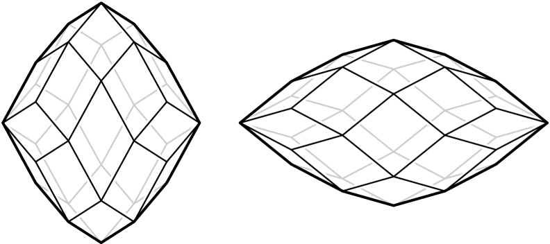
Remarkably, this reconstruction works across all combinatorial types and dimensions. That the reconstruction is only up to affine equivalence rather than isometry is due to examples such as rhombi and the zonotope in Figure˜5. In general, such flexibility via an affine transformation happens exactly if “the edge directions lie on a conic at infinity” (see [3, Proposition 4.2] or [5, Proposition 1.4]).

Lastly, the reconstruction permitted by Corollary˜3.8 is feasible in practice. This follows from a reformulation of Theorem˜3.2 as a semi-definite program, which can be solved in polynomial time. This is elaborated on in the alternative proof given in Appendix˜F.

4. Rigidity, tensegrity and reconstruction

Our reason for pursuing Theorem˜3.2 in Section˜3 was to transfer the proof of the simplex case (Theorem˜2.1) to general polytopes with the eventual goal of verifying the main conjecture and its corresponding “unique reconstruction version”:

Conjecture 1.2.

Given polytopes $P\subset\mathbb{R}^{d}$ and $Q\subset\mathbb{R}^{e}$ with common edge-graph. If

()

$0\in\operatorname{int}(Q)$ ,
()

edges in $Q$ are at most as long as in $P$ , and
()

vertex-origin distances in $Q$ are at least as large as in $P$ ,

then $P\simeq Q$ .

Conjecture 1.1.

A polytope $P$ with $0\in\operatorname{int}(P)$ is uniquely determined (up to isometry) by its edge-graph, edge lengths and vertex-origin distances.

In contrast to our formulation of Theorem˜3.2, both of the above conjectures are false when stated for a general graph embedding $q\colon V(G_{P})\to\mathbb{R}^{e}$ instead of $Q$ , even if we require $0\in\operatorname{int}\operatorname{conv}(q)$ . The following counterexample was provided by Joseph Doolittle [7]:

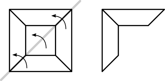
Example 4.1.

The 3-cube $P:=[-1,1]^{3}\subset\mathbb{R}^{3}$ is inscribed in a sphere of radius $\smash{\sqrt{3}}$ . Figure˜6 shows an inscribed embedding $q\colon V(G_{P})\to\mathbb{R}^{2}$ with the same circumradius and edge lengths, collapsing $G_{P}$ onto a path. In the circumcircle each edge spans an arc of length

2\sin^{-1}(1/\sqrt{3})\approx 70.5287^{\circ}>60^{\circ}.

The three edges therefore suffice to reach more than half around the circle. In other words, the convex hull of $q$ contains the circumcenter in its interior.

A full-dimensional counterexample in $\mathbb{R}^{3}$ can be obtained by interpreting $q$ as embedded in $\mathbb{R}^{2}\times\{0\}$ follows by a slight perturbation.

Potential fixes to the “graph embedding versions” of ˜1.1 and ˜1.2 are discussed in Section˜5.2.

While the general ˜1.2 will stay open, we are confident that our methods point the right way and highlight the essential difficulties. We overcome them in three relevant special cases, for some of which we actually can replace $Q$ with a graph embedding $q\colon V(G_{P})\to\mathbb{R}^{e}$ . Those are

()

$P$ and $q$ are centrally symmetric (Theorem˜4.4).
()

$q$ is a sufficiently small perturbation of $\operatorname{sk}(P)$ (Theorem˜4.5).
()

$P$ and $Q$ are combinatorially equivalent (Theorem˜4.7).

4.1. The remaining difficulty

On trying to generalize the proof of Theorem˜2.1 beyond simplices using Theorem˜3.2 we face the following difficulty: Theorem˜3.2 requires the $\alpha\in\Delta_{n}$ to be Wachspress coordinates of an interior point $x\in\operatorname{int}(P)$ , whereas in the proof of Theorem˜2.1 we use that $\alpha$ is a set of barycentric coordinates of $0\in$ $\operatorname{int}(Q)$ . While we have some freedom in choosing $x\in\operatorname{int}(P)$ , and thereby $\alpha\in\Delta_{n}$ , it is not clear that any such choice yields barycentric coordinates for $0\in\operatorname{int}(Q)$ . In fact, this is the only obstacle preventing us from proving ˜1.2 right away. For convenience we introduce the following map:

Definition 4.2.

Given polytopes $P\subset\mathbb{R}^{d}$ and $Q\subset\mathbb{R}^{e}$ , the Wachspress map $\phi\colon P\to Q$ is defined as follows: for $x\in P$ with Wachspress coordinates $\alpha(x)\in\Delta_{n}$ set

\phi(x):=\sum_{i}\alpha_{i}(x)q_{i}.

In cases where we are working with a graph embedding $q\colon V(G_{P})\to\mathbb{R}^{e}$ instead of $Q$ we have an analogous map $\phi\colon P\to\operatorname{conv}(q)$ .

Our previous discussion amounts to checking whether the origin is in the image of $\operatorname{int}(P)$ w.r.t. $\phi$ . While this could be reasonably true if $\dim P\geq\dim Q$ , it is certainly too much to hope for if $\dim P<\dim Q$ : the image of $\phi(\operatorname{int}(P))\subset Q$ is of a smaller dimension than $Q$ and easily “misses” the origin. Fortunately, we can ask for less, which we now formalize in (i) of the following lemma:

Lemma 4.3.

Let $P\subset\mathbb{R}^{d}$ be a polytope and $q\colon V(G_{P})\to\mathbb{R}^{e}$ some embedding. If

()

there exists an $x\in\operatorname{int}(P)$ with $\|\phi(x)\|\leq\|x\|$ (e.g. $\phi(x)=0$ ),
()

edges in $q$ are at most as long as in $P$ , and
()

vertex-origin distances in $q$ are at least as large as in $P$ ,

then $q\simeq\operatorname{sk}(P)$ (via an orthogonal transformation).

Proof.

Choose $x\in\operatorname{int}P$ with $\|\phi(x)\|\leq\|x\|$ , and note that its Wachspress coordinates $\alpha\in\operatorname{int}\Delta_{n}$ are strictly positive. In the remainder we follow closely the proof of Theorem˜2.1: consider the system of (in)equalities:

	$\displaystyle\sum_{i}\alpha_{i}\\|p_{i}\\|^{2}$	$\displaystyle=\Big{\\|}\sum_{i}\alpha_{i}p_{i}\Big{\\|}^{2}\!+\tfrac{1}{2}\sum_{i,j}\alpha_{i}\alpha_{j}\\|p_{i}-p_{j}\\|^{2}=\;\;\\|x\\|^{2}\;\;\;\,+\\|P\\|_{\alpha}^{2}$

	$\displaystyle\sum_{i}\alpha_{i}\\|q_{i}\\|^{2}$	$\displaystyle=\Big{\\|}\sum_{i}\alpha_{i}q_{i}\Big{\\|}^{2}\!+\tfrac{1}{2}\sum_{i,j}\alpha_{i}\alpha_{j}\\|q_{i}-q_{j}\\|^{2}\,=\\|\phi(x)\\|^{2}\,+\,\\|q\\|_{\alpha}^{2},$

where the two rows hold by simple computation and the vertical inequalities follow (from left to right) by (iii), (i), and (ii) + Theorem˜3.2 respectively. It follows that all inequalities are actually equalities. In particular, since $\alpha_{i}>0$ we find both $\|p_{i}\|$ $=$ $\|q_{i}\|$ for all $i\in V$ and $\|p_{i}-p_{j}\|=\|q_{i}-q_{j}\|$ for all $i,j\in V(G_{P})$ , establishing that $q$ and $\operatorname{sk}(P)$ are indeed isometric via an orthogonal transformation. ∎

The only way for Lemma˜4.3 (i) to fail is if $\|\phi(x)\|>\|x\|$ for all $x\in\operatorname{int}(P)$ . By (ii) and (iii) we have $\|\phi(x)\|=\|x\|$ whenever $x$ is a vertex or in an edge of $P$ , which makes it plausible that (i) should not fail, yet it seems hard to exclude in general.

In each of the three special cases of ˜1.2 discussed below we actually managed to verify $0\in\phi(\operatorname{int}(P))$ in order to apply Lemma˜4.3.

4.2. Central symmetry

Let $P\subset\mathbb{R}^{d}$ be centrally symmetric (more precisely, origin symmetric), that is, $P=-P$ . This induces an involution $\iota\colon V(G_{P})\to V(G_{P})$ with $p_{\iota(i)}=-p_{i}$ for all $i\in V(G_{P})$ . We say that an embedding $q\colon V(G_{P})\to\mathbb{R}^{d}$ of the edge-graph is centrally symmetric if $q_{\iota(i)}=$ $-q_{i}$ for all $i\in V(G_{P})$ .

Theorem 4.4 (centrally symmetric version).

Given a centrally symmetric polytope $P\subset\mathbb{R}^{d}$ and a centrally symmetric graph embedding $q\colon V(G_{P})\to\mathbb{R}^{e}$ , so that

()

edges in $q$ are at most as long as in $P$ , and
()

vertex-origin distances in $q$ are at least as large as in $P$ ,

then $q\simeq\operatorname{sk}(P)$ .

Proof.

Since $P$ is centrally symmetric, we have $0\in\operatorname{relint}(P)$ and we can find Wachspress coordinates $\alpha\in\operatorname{int}(\Delta_{n})$ of the origin in $P$ . Since the Wachspress coordinates are invariant under a linear transformation (as noted in Remark˜3.7 (ii)), it holds $\alpha_{i}=\alpha_{\iota(i)}$ . For the Wachspress map $\phi$ follow

\phi(0)=\tfrac{1}{2}\sum_{i\in V}\alpha_{i}q_{i}+\tfrac{1}{2}\sum_{i\in V}\alpha_{\iota(i)}q_{\iota(i)}=\tfrac{1}{2}\sum_{i\in V}\alpha_{i}q_{i}-\tfrac{1}{2}\sum_{i\in V}\alpha_{i}q_{i}=0,

The claim then follows via Lemma˜4.3 ∎

It is clear that Theorem˜4.4 can be adapted to work with other types of symmetry that uniquely fix the origin, such as irreducible symmetry groups.

Theorem˜4.4 has a natural interpretation in the language of classical rigidity theory, where it asserts the universal rigidity of a certain tensegrity framework. In this form it was proven up to dimension three by Connelly [4, Theorem 5.1]. We elaborate further on this in Section˜5.3.

It is now tempting to conclude the unique reconstruction version of Theorem˜4.4, answering ˜1.1 for centrally symmetric polytope. There is however a subtlety: our notion of “central symmetry” for the graph embedding $q\colon V(G_{P})\to\mathbb{R}^{e}$ as used in Theorem˜4.4 has been relative to $P$ , in that it forces $q$ to have the same pairs of antipodal vertices as $P$ . It is however not true that any two centrally symmetric polytopes with the same edge-graph have this relation. David E. Speyer [25] constructed a 12-vertex 4-polytope whose edge-graph has an automorphism that does not preserve antipodality of vertices.

4.3. Local uniqueness

Given a polytope $P\subset\mathbb{R}^{d}$ consider the space

\mathcal{E}_{P}:=\{q:V(G_{P})\to\mathbb{R}^{d}\}

of $d$ -dimensional embeddings of $G_{P}$ . We then have $\operatorname{sk}(P)\in\mathcal{E}_{P}$ . Since $\mathcal{E}_{P}\cong\leavevmode\nobreak\ \mathbb{R}^{n\times d}$ (in some reasonable sense) we can pull back a metric $\mu\colon\mathcal{E}_{P}\times\mathcal{E}_{P}\to\mathbb{R}_{+}$ .

Theorem 4.5 (local version).

Given a polytope $P\subset\mathbb{R}^{d}$ with $0\in\operatorname{int}(P)$ , there exists an $\epsilon>0$ with the following property: if $q\colon V(G_{P})\to\mathbb{R}^{d}$ is an embedding with

()

$q$ is $\epsilon$ -close to $\operatorname{sk}(P)$ , i.e., $\mu(q,\operatorname{sk}(P))<\epsilon$ ,
()

edges in $q$ are at most as long as in $P$ , and
()

vertex-origin distances in $q$ are at least as large as in $P$ ,

then $q\simeq\operatorname{sk}(P)$ .

Theorem˜4.5 as well can be naturally interpreted in the language of rigidity theory (see Section˜5.3). The proof below makes no use of this language.

In order to prove Theorem˜4.5 we again show $0\in\phi(\operatorname{int}(P))$ , which requries more work this time: since $0\in\operatorname{int}(P)$ , there exists an $\epsilon$ -neighborhood $B_{\epsilon}(0)\subset P$ of the origin. The hope is that for a sufficiently small perturbation of the vertices of $P$ the image of $B_{\epsilon}(0)$ under $\phi$ is still a neighborhood of the origin.

This hope is formalized and verified in the following lemma, which we separated from the proof of Theorem˜4.5 to reuse it in Section˜4.4. Its proof is standard and is included in Appendix˜D:

Lemma D.1.

Let $K\subset\mathbb{R}^{d}$ be a compact convex set with $0\in\operatorname{int}(K)$ and $f\colon K\times[0,1]$ $\to\mathbb{R}^{d}$ a homotopy with $f(\kern 0.70007pt\cdot\kern 0.70007pt,0)=\operatorname{id}_{K}$ . If the restriction $f|_{\partial K}\colon\partial K\times[0,1]\to\mathbb{R}^{d}$ yields a homotopy of $\partial K$ in $\mathbb{R}^{d}\setminus\{0\}$ , then $0\in\operatorname{int}f(K,1)$ .

In other words: if a “well-behaved” set $K$ contains the origin in its interior, and it is deformed so that its boundary never crosses the origin, then the origin stays inside.

Proof of Theorem˜4.5.

Since $0\in\operatorname{int}(P)$ there exists a $\delta>0$ with $B_{\delta}(0)\subset P$ .

Fix some compact neighborhood $N\subset\mathcal{E}_{P}$ of $\operatorname{sk}(P)$ . Then $N\times P$ is compact in $\mathcal{E}_{P}\times\mathbb{R}^{d}$ and the map

N\times P\to\mathbb{R}^{d},\;\;(q,x)\mapsto\phi_{q}(x):=\sum_{i}\alpha_{i}(x)q_{i}

is uniformly continuous: there exists an $\epsilon>0$ so that whenever $\mu(q,q^{\prime})+\|x-x^{\prime}\|<\epsilon$ , we have $\|\phi_{q}(x)-\phi_{q^{\prime}}(x^{\prime})\|<\delta/2$ . We can assume that $\epsilon$ is sufficiently small, so that $B_{\epsilon}(\operatorname{sk}(P))\subset N$ . We show that this $\epsilon$ satisfies the statement of the theorem.

Suppose that $q$ is $\epsilon$ -close to $\operatorname{sk}(P)$ , then

\mu(\operatorname{sk}(P),q)+\|x-x\|<\epsilon\;\,\implies\;\,\|x-\phi_{q}(x)\|=\|\phi_{\operatorname{sk}(P)}(x)-\phi_{q}(x)\|<\delta/2.

The same is true when replacing $q$ by any linear interpolation $q(t):=(1-t)\operatorname{sk}(P)+tq$ with $t\in[0,1]$ . Define the following homotopy:

f\colon B_{\delta}(0)\times[0,1]\to\mathbb{R}^{d},\quad(x,t)\mapsto\phi_{q(t)}(x).

We have $f(\kern 0.70007pt\cdot\kern 0.70007pt,0)=\operatorname{id}$ . That is, if $x\in\partial B_{\delta}(0)$ then $\|f(x,0)\|=\delta$ , as well as

\|f(x,t)\|\geq\|f(x,0)\|-\|f(x,0)-f(x,t)\|\geq\delta-\delta/2=\delta/2,

and $f(x,t)\not=0$ for all $t\in[0,1]$ . Since $B_{\delta}(0)$ is compact and convex, the homotopy $f$ satisfies the conditions of Lemma˜D.1 and we conclude $0\in f(B_{\delta}(0),1)=\phi_{q}(B_{\delta}(0))$ $\subseteq\phi_{q}(\operatorname{int}(P))$ . Then $q\simeq\operatorname{sk}(P)$ follows via Lemma˜4.3. ∎

The polytope $P$ in Theorem˜4.5 is assumed to be full-dimensional. This is necessary, since allowing $\operatorname{sk}(P)$ to deform beyond its initial affine hull already permits counterexamples such as shown in Figure˜7. Even restricting to deformations with $0\in\operatorname{int}\operatorname{conv}(q)$ is not sufficient, as shown in the next example:

Example 4.6.

Consider the 3-cube as embedded in $\mathbb{R}^{3}\times\{0\}\subset\mathbb{R}^{3}\times\mathbb{R}^{2}\cong\mathbb{R}^{5}$ . Let $p_{1},...,p_{8}\in\mathbb{R}^{3}$ $\times$ $\{0\}$ be its vertices, and let $q_{1},...,q_{8}\in\{0\}\times\mathbb{R}^{2}$ be the vertices as embedded in Figure˜6 (on the right). Since both share the same edge lengths and vertex-origin distances, so does the embedding $tp+sq$ whenever $t^{2}+s^{2}=1$ . Observe further that for both $p_{i}$ and $q_{i}$ the origin can be written as a convex combination using the same coefficients $\alpha\in\Delta_{n}$ (use an $\alpha$ with $\alpha_{i}=\alpha_{j}$ whenever $p_{i}=-p_{j}$ ). It follows $0\in$ $\operatorname{int}\operatorname{conv}(tp+sq)$ .

4.4. Combinatorially equivalent polytopes

In this section we consider combinatorially equivalent polytopes $P,Q\subset\mathbb{R}^{d}$ and prove the following:

Theorem 4.7 (combinatorial equivalent version).

Let $P,Q\subset\mathbb{R}^{d}$ be combinatorially equivalent polytopes so that

()

$0\in\operatorname{int}(Q)$
()

edges in $Q$ are at most as long as in $P$ , and
()

vertex-origin distances in $Q$ are at least as large as in $P$ .

Then $P\cong Q$ .

In particular, since the combinatorics of polytopes up to dimension three is determined by the edge-graph, this proves ˜1.2 for $d,e\leq 3$ .

Once again the proof uses Lemma˜4.3. Since $0\in\operatorname{int}(Q)$ , we can verify $0\in\phi(\operatorname{int}(P))$ by showing that the Wachspress map $\phi\colon P\to Q$ is surjective. This statement is of independent interest, since the question whether $\phi$ is bijective is a well-known open problem for $d\geq 3$ (see ˜5.11). Our proof of surjectivity uses Lemma˜D.1 and the following:

Lemma 4.8.

Given a face $\sigma\in\mathcal{F}(P)$ , the Wachspress map $\phi$ sends $\sigma$ onto the corresponding face $\sigma_{Q}\in\mathcal{F}(Q)$ . In particular, $\phi$ sends $\partial P$ onto $\partial Q$ .

Proof.

Given a point $x\in\operatorname{relint}(\sigma)$ with Wachspress coordinates $\alpha\in\Delta_{n}$ , the coefficient $\alpha_{i}$ is non-zero if and only if the vertex $p_{i}$ is in $\sigma$ (Remark˜3.7 (i)). The claim $\phi(x)\in\sigma_{Q}$ follows immediately. ∎

Lemma 4.9.

The Wachspress map $\phi\colon P\to Q$ is surjective.

Proof.

We proceed by induction on the dimension $d$ of $P$ . For $d=1$ the Wachspress map is linear and the claim is trivially true. For $d>1$ recall that $\phi$ sends $\partial P$ to $\partial Q$ (by Lemma˜4.8). By induction hypothesis, $\phi$ is surjective on each proper face, thus surjective on all of $\partial P$ .

To show surjectivity in the interior, we fix $x\in\operatorname{int}(Q)$ ; we show $x\in\operatorname{im}\phi$ . Let $\psi\colon Q\to P$ be the Wachspress map in the other direction (which is usually not the inverse of $\phi$ ) and define $\rho:=\phi\circ\psi\colon Q\to Q$ . Note that by Lemma˜4.8 $\rho$ sends each face of $Q$ to itself and is therefore homotopic to the identity on $Q$ via the following linear homotopy:

f\colon Q\times[0,1]\to Q,\;(y,t)\mapsto(1-t)x+t\rho(x).

Since faces of $Q$ are closed under convex combination, $f(\kern 0.70007pt\cdot\kern 0.70007pt,t)$ sends $\partial Q$ to itself for all $t\in[0,1]$ . Thus, $f$ satisfies the assumptions of Lemma˜D.1 (with $K$ chosen as $Q$ ), and therefore $x\in f(Q,1)=\operatorname{im}\rho\subset\operatorname{im}\phi$ . ∎

The proof of Theorem˜4.7 follows immediately:

Proof of Theorem˜4.7.

Since $0\in\operatorname{int}(Q)$ and the Wachspress map $\phi\colon P\to Q$ is surjective (by Lemma˜4.9), there exists $x\in P$ with $\phi(x)=0$ . Since $\phi(\partial P)=\partial Q$ (by Lemma˜4.8), we must have $x\in\operatorname{int}(P)$ . $P\simeq Q$ then follows via Lemma˜4.3. ∎

Corollary 4.10.

A polytope with the origin in its interior is uniquely determined by its face-lattice, its edge lengths and its vertex-origin distances.

If the origin lies not in $P$ then a unique reconstruction is not guaranteed (recall Figure˜3). However, if $0\in\partial P$ then we can say more. Recall the tangent cone of $P$ at a face $\sigma\in\mathcal{F}(P)$ :

T_{P}(\sigma):=\operatorname{cone}\{x-y\mid x\in P,\,y\in\sigma\}.

Theorem 4.11.

Let $P,Q\subset\mathbb{R}^{d}$ be combinatorially equivalent polytopes with the following properties:

()

$0\in\operatorname{relint}(\sigma_{Q})$ for some face $\sigma_{Q}\in\mathcal{F}(Q)$ , $\sigma_{P}$ is the corresponding face in $P$ , and $P$ and $Q$ have isometric tangent cones at $\sigma_{P}$ and $\sigma_{Q}$ .
()

edges in $Q$ are at most as long as in $P$ .
()

vertex-origin distances in $Q$ are at least as large as in $P$ .

Then $P\cong Q$ .

Property (i) is always satisfied if, for example, $\sigma_{Q}$ is a facet of $Q$ , or if $\sigma_{Q}$ is a face of codimension two at which $P$ and $Q$ agree in the dihedral angle.

Proof.

The proof is by induction on the dimension $d$ of the polytopes. The induction base $d=1$ is clearly satisfied. In the following we assume $d\geq 2$ .

Note first that we can apply Theorem˜4.7 to $\sigma_{P}$ and $\sigma_{Q}$ to obtain $\sigma_{P}\simeq\sigma_{Q}$ via an orthogonal transformation $T\colon\mathbb{R}^{d}\to\mathbb{R}^{d}$ , in particular $0\in\operatorname{relint}(\sigma_{P})\subseteq P$ . By (i) this transformation extends to the tangent cones at these faces. Let $F_{1,Q},...,F_{m,Q}\in\mathcal{F}_{d-1}(Q)$ be the facets of $Q$ that contain $\sigma_{Q}$ , and let $F_{1,P},...,F_{m,P}\in\mathcal{F}_{d-1}(P)$ be the corresponding facets in $P$ . Then $F_{i,P}$ and $F_{i,Q}$ too have isometric tangent cones at $\sigma_{P}$ resp. $\sigma_{Q}$ , and $F_{i,P}\simeq F_{i,Q}$ follows by induction hypothesis.

Now choose a point $x_{Q}\in\mathbb{R}^{d}$ beyond the face $\sigma_{Q}$ (i.e., above all facet-defining hyperplanes that contain $\sigma_{Q}$ , and below the others) so that $x_{P}:=Tx_{Q}$ is beyond the face $\sigma_{P}$ . Consider the polytopes $Q^{\prime}:=\operatorname{conv}(Q\cup\{x_{Q}\})$ and $P^{\prime}:=\operatorname{conv}(P\cup\{x_{P}\})$ . Since $x_{Q}$ lies beyond $\sigma_{Q}$ , each edge of $Q^{\prime}$ is either an edge of $Q$ , or is an edge between $x_{Q}$ and a vertex of some facet $F_{i,Q}$ ; and analogously for $P^{\prime}$ . The lengths of edges incident to $x_{Q}$ depend only on the shape of the tangent cone and the shapes of the facets $F_{i,Q}$ , hence are the same for corresponding edges in $P^{\prime}$ . Thus, $P^{\prime}$ and $Q^{\prime}$ satisfy the preconditions of Theorem˜4.7, and we have $P^{\prime}\simeq Q^{\prime}$ .

Finally, as $x_{Q}\to 0$ , we have $Q^{\prime}\to Q$ and $P^{\prime}\to P$ (in the Hausdorff metric), which shows that $P\simeq Q$ . ∎

Thus, if the origin lies in the interior of $P$ or a facet of $P$ then Theorem˜4.7 applies. If the origin lies in a face of codimension three, then counterexamples exist.

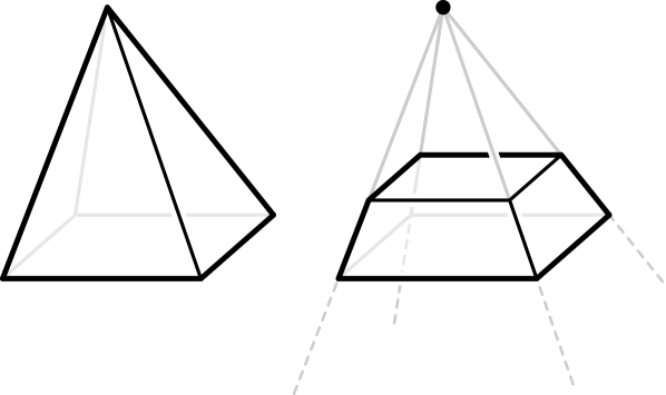
Example 4.12.

Consider the pentagons from Figure˜3 as lying in the plane $\mathbb{R}^{2}\times\{1\}$ , with their former origins now at $(0,0,1)$ . Consider the pyramids

P^{*}:=\operatorname{conv}(P\cup\{0\})\quad\text{and}\quad Q^{*}:=\operatorname{conv}(Q\cup\{0\}).

These polytopes have the origin in a vertex (a face of codimension three), have the same edge-graphs, edge lengths and vertex-origin distances, yet are not isometric. Examples with the origin in a high-dimensional face of codimension three can be constructed by considering prisms over $P^{*}$ resp. $Q^{*}$ .

We do not know whether Theorem˜4.7 holds if the origin lies in a face of codimension two (see ˜5.13).

4.5. Inscribed polytopes

It is worthwhile to formulate versions of Theorem˜4.7 for inscribed polytopes, that is, polytopes where all vertices lie on a common sphere – the circumsphere. For inscribed polytopes we can write down a direct monotone relation between edge lengths and the circumradius.

Corollary 4.13 (inscribed version).

Given two combinatorially equivalent polytopes $P,Q\subset\mathbb{R}^{d}$ so that

()

$P$ and $Q$ are inscribed in spheres of radii $r_{P}$ and $r_{Q}$ respectively,
()

$Q$ contains its circumcenter in the interior, and
()

edges in $Q$ are at most as long as in $P$ ,

Then $r_{P}\geq r_{Q}$ , with equality if and only if $P\simeq Q$ .

Proof.

Translate $P$ and $Q$ so that both circumcenters lie at the origin. Suppose that $r_{P}\leq r_{Q}$ . Then all preconditions of Theorem˜4.7 are satisfied, which yields $P\simeq Q$ , hence $r_{P}=r_{Q}$ . ∎

This variant in particular has already found an application in proving the finitude of so-called “compact sphere packings” with spheres of only finitely many different radii [20].

Interestingly, the corresponding “unique reconstruction version” does not require any assumptions about the location of the origin or an explicit value for the circumradius. In fact, we do not even need to apply our results, as it already follows from Cauchy’s rigidity theorem (Theorem˜B.1).

Corollary 4.14.

An inscribed polytope of a fixed combinatorial type is uniquely determined, up to isometry, by its edge lengths.

Proof.

The case $d=2$ is straightforward: given any circle, there is only a single way (up to isometry) to place edges of prescribed lengths. Also, there is only a single radius for the circle for which the edges reach around the circle exactly once and close up perfectly. This proves uniqueness for polygons.

If $P$ is of higher dimension then its 2-dimensional faces are still inscribed, have prescribed edge lengths, and by the 2-dimensional case above, corresponding 2-faces in $P$ and $Q$ are therefore isometric. Then $P\simeq Q$ follows from Cauchy’s rigidity theorem (Theorem˜B.1). ∎

5. Conclusion, further notes and many open questions

We conjectured that a convex polytope is uniquely determined up to isometry by its edge-graph, edge lengths and the collection of distances between its vertices and some interior point, across all dimensions and combinatorial types (˜1.1). We also posed a more general conjecture expressing the idea that polytope skeleta, given their edge lengths, are maximally expanded (˜1.2). We developed techniques based on Wachspress coordinates and the so-called Izmestiev matrix that led to us to resolve three relevant special cases: centrally symmetric polytopes (Theorem˜4.4), small perturbations (Theorem˜4.5), and combinatorially equivalent polytopes (Theorem˜4.7). We feel confident that our approach already highlights the essential difficulties in verifying the general case.

In this section we collected further thoughts on our results, notes on connections to the literature, as well as many questions and future research directions.

5.1. Consequences of the conjectures

˜1.1 vastly generalizes several known “reconstruction from the edge-graph” results. The following is a special case of ˜1.1: an inscribed polytopes with all edges of the same length would be uniquely determined by its edge-graph. This includes the following special cases:

•

The reconstruction of matroids from their base exchange graph: a matroid can be identified with its matroid base polytopes, which is a 01-polytopes (hence inscribed) and has all edges of length $\sqrt{2}$ . This reconstruction has been initially proven in [14] and recently rediscovered in [24].
•

The reconstruction of simultaneously vertex- and edge-transitive polytopes from their edge-graph: this was proven in [34, 36], essentially using the tools of this article.

It would imply an analogous reconstruction from the edge-graph for classes of polytopes such as the uniform polytopes or higher-dimensional inscribed Johnson solids [16].

Secondly, a positive answer to ˜1.1 would also resolve Question 6.6 in [35] on whether the metric coloring can capture the Euclidean symmetries of a polytope.

5.2. ˜1.2 for graph embeddings

In Example˜4.1 we show that ˜1.2 does not hold when replacing $Q$ by some more general graph embedding $q\colon V(G_{P})\to\mathbb{R}^{e}$ of $G_{P}$ , even if $0\in\operatorname{int}\operatorname{conv}(q)$ .

Our intuition for why this fails, and also what distinguishes it from the setting of our conjectures and the verified special cases is, that the embedding of Example˜4.1 does not “wrap around the origin” properly. It is not quite clear what this means for an embedding of a graph, except that it feels right to assign this quality to polytope skeleta, to embeddings close to them, and also to centrally symmetric embeddings.

One possible formalization of this idea is expressed in the conjecture below, that is even stronger than ˜1.2 (the idea is due to Joseph Doolittle):

Conjecture 5.1.

Given a polytope $P\subset\mathbb{R}^{d}$ and a graph embedding $q\colon V(G_{P})\to\mathbb{R}^{e}$ of its edge-graph $G_{P}$ , so that

()

for each vertex $i\in V(G_{P})$ the cone

$C_{i}:=q_{i}+\operatorname{cone}\{q_{j}-q_{i}\mid ij\in E(G_{P})\}$

contains the origin in its interior,
()

edges in $q$ are at most as long as in $P$ , and
()

vertex-origin distances in $q$ are at least as large as in $P$ ,

then $\operatorname{sk}(P)\simeq q$ .

Note that since $\bigcap_{i}C_{i}\subseteq\operatorname{conv}(q)$ , (i) already implies $0\in\operatorname{int}\operatorname{conv}(q)$ .

5.3. Classical rigidity of frameworks

We previously commented on a natural interpretation of Theorem˜4.4 and Theorem˜4.5 in the language of classical rigidity theory (we refer to [6] for any rigidity specific terminology used below).

Consider the edges of $P$ as cables that can contract but not expand, and connect all vertices of $P$ to the origin using struts that can expand but not contract. This is known as a tensegrity framework, and we shall call it the tensegrity of $P$ . Theorem˜4.5 then asserts that these tensegrities are always (locally) rigid.

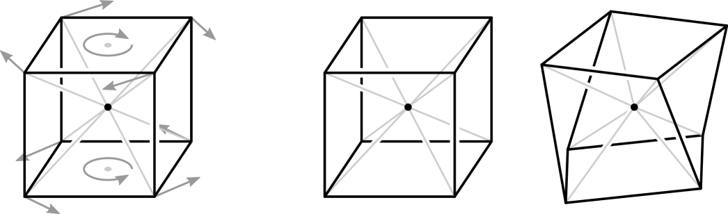
Using the language of rigidity, a number of natural follow up questions arise. So it turns out that swapping cables and struts does not necessarily preserve rigidity; see Figure˜8 for an example. As a consequence, the tensegrity of a polytope is not necessarily infinitesimally rigid, because infinitesimally rigid frameworks stay rigid under swapping cables and struts.

Lacking first-order rigidity, we might ask for higher-order rigidity instead:

Question 5.2.

Is the tensegrity of a polytope always second-order rigid, or perhaps even prestress stable?

For an interpretation of Theorem˜4.4 as a tensegrity framework, consider a cable at each edge as before, but each central strut now connects a vertex $p_{i}$ to its antipodal counterpart $-p_{i}$ , and is fixed in its center to the origin. Theorem˜4.4 then asserts that this tensegrity framework is universally rigid, i.e., it has a unique realization across all dimensions.

Here too, swapping cables and struts does not preserve universal or even global rigidity (see Figure˜9). It does not preserve local rigidity either (see Example˜5.3).

Example 5.3.

Consider the 4-cube with its “top” and “bottom” facets (which are 3-cubes) embedded in the hyperplanes $\mathbb{R}^{3}\times\{\pm 1\}$ respectively. We flex the skeleton as follows: deform the top facet as shown in Figure˜8, and the bottom facet so as to keep the framework centrally symmetric, while keeping both inside their respective hyperplanes. The edge struts inside the facets become longer, and the edge struts between the facets have previously been of minimal length between the hyperplanes, can therefore also only increase in length. The lengths of the central cables stay the same.

As a consequence, the centrally symmetric tensegrity frameworks too are not necessarily infinitesimally rigid.

5.4. Schlegel diagrams

Yet another interpretation of the frameworks discussed in Section˜5.3 is as skeleta of special Schlegel diagrams, namely, of pyramids whose base facet is the polytope $P$ . It is then natural to ask whether a general Schlegel diagram is rigid as well (this was brought up by Raman Sanyal).

The question of rigidity for Schlegel diagrams is already interesting in dimension two, that is, for Schlegel diagrams of 3-polytopes. The edge-graphs of many 3-polytopes are too sparse to be generically rigid in $\mathbb{R}^{2}$ , and so one might expect that most of their Schlegel diagrams are flexible. Indeed, flexible Schlegel diagrams exist (see Figure˜11, left).

Surprisingly however, this seems to be the exception rather than the rule. For example, we believe that Schlegel diagrams of $(2n+1)$ -gonal prisms are always rigid (see Figure˜11, right). Since Schlegel diagrams are very special realizations (they are projections of convex objects), the generic ones among them might very well be rigid. This is not clear so far.

Question 5.4.

Is a generic Schlegel diagram rigid?

Above we considered Schlegel diagrams as bar-joint frameworks. If we consider them as tensegrity frameworks then it is easy to find generically flexible examples (see Figure˜12). Schlegel diagrams are also not necessarily globally rigid (see Figure˜13).

5.5. Stoker’s conjecture

Stoker’s conjecture asks whether the dihedral angles of a polytope determine its face angles, and thereby its overall shape to some degree. Recall that dihedral angles are the angle at which facets meet in faces of codimension two, whereas face angles are the dihedral angles of the facets. Stoker’s conjecture was asked in 1968 [26], and a proof was claimed recently by Wang and Xie [29]:

Theorem 5.5 (Wang-Xie, 2022).

Let $P_{1}$ and $P_{2}$ be two combinatorially equivalent polytopes such that corresponding dihedral angles are equal. Then all corresponding face angles are equal as well.

Our results allow us to formulate a semantically similar statement. The following is a direct consequence of Corollary˜4.10 when expressed for the polar dual polytope:

Corollary 5.6.

Let $P_{1}$ and $P_{2}$ be two combinatorially equivalent polytopes such that corresponding dihedral angles and facet-origin distances are equal. Then $P_{1}\simeq P_{2}$ .

While the assumptions in Corollary˜5.6 are unlike stronger compared to Stoker’s conjecture (we require facet-origin distances), we also obtain isometry instead of just identical face angles. While related, we are not aware that either of Theorem˜5.5 or Corollary˜5.6 follows from the other one easily.

5.6. Pure edge length constraints

Many polytopes cannot be reconstructed up to isometry from their edge-graph and edge lengths alone (recall Figure˜1). However, for all we know the following is open:

Question 5.7.

Is the combinatorial type of a polytope uniquely determined by its edge-graph and edge lengths?

This alone would already prove ˜1.1 (by Corollary˜4.10). It would also imply a positive answer to the following:

Question 5.8.

Is a polytope uniquely determined up to isometry by its 2-skeleton (i.e., the face-lattice cut off at, but including dimension two) and the shape of each 2-face?

Note that this is a particular strengthening of Cauchy’s rigidity theorem, which requires the face-lattice to be prescribed in its entirety, rather than on some lower levels only.

Let us now fix the combinatorial type. We are aware of three types of polytopes that are not determined (up to isometry) by their face-lattice and edge lengths:

()

$n$ -gons with $n\geq 4$ .
()

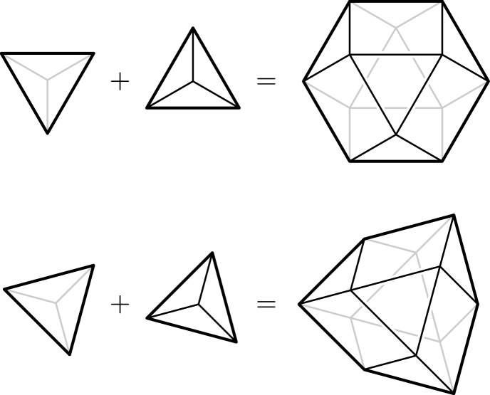
Minkowski sums: if $P=Q+R$ and $Q$ and $R$ are generically oriented w.r.t. each other, then a slight reorientation of the summands changes the shape of $P$ but keeps its edge lengths (see Figure˜14).
()

polytopes having all edge directions on a “conic at infinity”: this implies an affine flex (see [5]). This is most easily implemented for zonotopes (recall Figure˜5), but happens for other polytopes as well, such as 3-polytopes with up to five edge directions (see Figure˜15).

We are not aware of other examples of polytopes that flex in this way and so we wonder whether this is already a full characterization.

Question 5.9.

If a polytope is not determined up to isometry by its combinatorial type and edge lengths, is it necessarily a polygon, a non-trivial Minkowski sum or has all its edge directions on a conic at infinity? Is this true at least up to dimension three?

In how far a 3-polytope is determined by local metric data at its edges was reportedly discussed in an Oberwolfach question session (as communicated by Ivan Izmestiev on MathOverflow [33]), where the following more general question was asked:

Question 5.10.

Given a simplicial 3-polytope and at each edge we prescribe either the length or the dihedral angle, in how far does this determine the polytope?

Having length constraints at every edge determines a simplicial polytope already up to isometry via Cauchy’s rigidity theorem (Theorem˜B.1). The angles-only version is exactly the 3-dimensional Stoker’s conjecture (Section˜5.5). We are not aware that this question has been addressed in the literature beyond these two extreme cases.

Note also that ˜5.10 is stated for simplicial 3-polytopes, but actually includes general 3-polytopes via a trick: if $P$ is not simplicial, triangulate every 2-face, and at each new edge created in this way prescribe a dihedral angle of $180^{\circ}$ to prevent the faces from folding at it.

5.7. Injectivity of the Wachspress map $\boldsymbol{\phi}$

In Lemma˜4.9 we proved that the Wachspress map $\phi\colon P\to Q$ (cf. Definition˜4.2) between combinatorially equivalent polytopes is surjective. In contrast, the injectivity of the Wachspress map has been established only in dimension two by Floater and Kosinka [10] and is conjectured for all $d\geq 3$ .

Conjecture 5.11.

The Wachspress map $\phi\colon P\to Q$ is injective.

If true, the Wachspress map would provide an interesting and somewhat canonical homeomorphism (in fact, a rational map, see [31]) between any two combinatorially equivalent polytopes.

5.8. What if $\boldsymbol{0\not\in\mathrm{int}(Q)}$ ?

If $0\not\in Q$ then Figures˜4 and 3 show that our conjectures fail. We do however not know whether in the “unique reconstruction” case the number of solutions would be finite.

Question 5.12.

Given edge-graph, edge lengths and vertex-origin distances, are there only finitely many polytopes with these parameters?

This is in contrast to when we replace $Q$ with a graph embedding $q\colon V(G_{P})\to\mathbb{R}^{e}$ , which can have a continuum of realizations (see Figure˜16).

In Section˜4.4 we showed that reconstruction from the face-lattice, edge lengths and vertex-origin distances is possible even if the origin lies only in the inside of a facet of $P$ , but that it can fail if it lies in a face of codimension three. We do not know what happens for a face of codimension two.

Question 5.13.

Is a polytope uniquely determined by its face-lattice, edge lengths and vertex-origin distances if the origin is allowed to lie in the inside of faces of codimension $0,1$ and $2$ ?

Appendix A Perron-Frobenius theory

The following fragment of the Perron-Frobenius theorem is relevant to this article. Recall that a matrix is irreducible if no simultaneous row-column permutation brings it in a block-diagonal form with more than one block; or equivalently, if it is not the (weighted) adjacency matrix of a disconnected graph. See also [11].

Theorem A.1 (Perron-Frobenius).

Let $M\in\mathbb{R}^{n\times n}$ be a non-negative irreducible symmetric matrix, then

()

the largest eigenvalue $\theta$ of $M$ is positive and has multiplicity one.
()

there is a $\theta$ -eigenvector $z\in\mathbb{R}^{n}$ with strictly positive entries.

Appendix B Cauchy’s rigidity theorem

Cauchy’s famous rigidity theorem was initially formulated in dimension three and is often quoted briefly as follows:

3-polytopes with isometric faces are themselves isometric.

Generalizations to higher dimensions have been proven by Alexandrov [1] where one assumes isometric facets to conclude global isometry (see also its proof in [23]). We state a rigorous version that only requires isometric 2-faces and that can be easily derived from the facet versions using induction by dimension:

Theorem B.1 (Cauchy’s rigidity theorem, version with 2-faces).

Given two combinatorially equivalent polytopes $P,Q\subset\mathbb{R}^{d}$ and a face-lattice isomorphism $\phi\colon\mathcal{F}(P)\to\mathcal{F}(Q)$ . If $\phi$ extends to an isometry on every 2-face $\sigma\in\mathcal{F}_{2}(P)$ , then $\phi$ extends to an isometry on all of $P$ , that is, $P\simeq Q$ .

Appendix C Some linear algebra

Theorem C.1.

Given two matrices $A\in\mathbb{R}^{d\times n}$ and $B\in\mathbb{R}^{d\times m}$ with $\operatorname{span}B\subseteq\operatorname{span}A$ , there exists a linear transformation $T\colon\mathbb{R}^{n}\to\mathbb{R}^{m}$ with $TA^{\top}=B^{\top}$ .

Proof.

Set $U_{A}:=\operatorname{span}A$ and $d_{A}:=\dim U_{A}=\operatorname{rank}A$ . Respectively, set $U_{B}:=\operatorname{span}B\subset U_{A}$ and $d_{B}:=\dim U_{B}=\operatorname{rank}B$ . We can assume that the columns of $A$ and $B$ are sorted so that $a_{1},...,a_{d_{A}}\in U_{A}$ form a basis, and likewise $b_{1},...,b_{d_{B}}\in U_{B}$ form a basis. Let $\tilde{T}\colon U_{A}\to U_{B}$ be the uniquely determined linear map that maps $\tilde{T}a_{i}=b_{i}$ for $i\in\{1,...,d_{B}\}$ and $\tilde{T}a_{i}=0$ for $i\in\{d_{B}+1,...,d_{A}\}$ . Then $\tilde{T}A=B$ .

The Moore-Penrose pseudo inverse $A^{\dagger}\in\mathbb{R}^{n\times d}$ of $A$ satisfies $AA^{\dagger}=\pi_{U_{A}}$ , where $\pi_{U_{A}}$ is the orthogonal projection onto $U_{A}$ . We set $T:=(A^{\dagger}\tilde{T}A)^{\top}$ and verify

TA^{\top}=(AT^{\top})^{\top}=(AA^{\dagger}\tilde{T}A)^{\top}=(\pi_{U_{A}}\tilde{T}A)^{\top}=(\pi_{U_{A}}B)^{\top}=B^{\top},

where for the last equality we used that all columns of $B$ are already in $U_{A}$ and the projection acts as identity. ∎

Appendix D A topological argument

Lemma D.1.

Let $K\subset\mathbb{R}^{d}$ be a compact convex set, $x\in\operatorname{int}(K)$ a point and $f\colon K\times[0,1]\to\mathbb{R}^{d}$ a homotopy with $f(\kern 0.70007pt\cdot\kern 0.70007pt,0)=\operatorname{id}_{K}$ . If the restriction $f|_{\partial K}\colon\partial K\times[0,1]\to\mathbb{R}^{d}$ yields a homotopy of $\partial K$ in $\mathbb{R}^{d}\setminus\{x\}$ , then $x\in\operatorname{int}f(K,1)$ .

Proof.

Suppose that $x\not\in\operatorname{int}f(K,1)$ . Since $\partial f$ is a homotopy in $\mathbb{R}^{d}\setminus\{x\}$ , we actually have $x\not\in f(K,1)$ . We derive a contradiction.

Construct a map $g\colon K\to\partial K$ as follows: for $y\in K$ consider the unique ray emanating from $x$ passing through $f(y,1)$ . Let $g(x)$ be the unique intersection of this ray with $\partial K$ . Likewise, construct the map $h\colon\partial K\times[0,1]\to\partial K$ : for $y\in\partial K$ and $t\in[0,1]$ , let $h(y,t)$ be the intersection of $\partial K$ with the unique ray emanating from $x$ and passing through $f(y,t)$ . Note that $h(\kern 0.70007pt\cdot\kern 0.70007pt,0)=\operatorname{id}_{\partial K}$ and $h(\kern 0.70007pt\cdot\kern 0.70007pt,1)=g|_{\partial K}$ . In other words, $g|_{\partial K}$ is homotopic to the identity on $\partial K$ .

The existence of such a map $g\colon K\to\partial K$ is a well-known impossibility. This can be quickly shown by considering the following commutative diagram (left) and the diagram induced on the $\mathbb{Z}$ -homology groups (right):

Since $g|_{\partial K}$ is homotopic to the identity, the arrow $(g|_{\partial K})_{*}$ is an isomorphism, and so must be the arrows above it. This is impossible because

H_{d-1}(\partial K)=\mathbb{Z}\not=0=H_{d-1}(K).

∎

Appendix E Euler’s homogeneous function theorem

Theorem E.1 (Euler’s homogeneous function theorem).

Let $f\colon\mathbb{R}^{n}\to\mathbb{R}$ be a homogeneous function of degree $d\geq 1$ i.e., $f(t\mathbf{x})=t^{d}f(\mathbf{x})$ for all $t\geq 0$ . Then

\sum_{i}x_{i}\frac{\partial f(\mathbf{x})}{\partial x_{i}}=d\cdot f(\mathbf{x}).

Proof.

Differentiate both sides of $f(t\mathbf{x})=t^{d}f(\mathbf{x})$ w.r.t. $t$

dt^{d-1}f(\mathbf{x})=\frac{\partial}{\partial t}(t^{d}f(\mathbf{x}))=\frac{\partial}{\partial t}f(t\mathbf{x})=\sum_{i}\frac{\partial f(t\mathbf{x})}{\partial(tx_{i})}\frac{\partial(tx_{i})}{\partial t}=\sum_{i}x_{i}\frac{\partial f(t\mathbf{x})}{\partial(tx_{i})}

and evaluate at $t=1$ . ∎

Appendix F An alternative proof of Theorem˜3.2 using semi-definite optimization

The following proof of Theorem˜3.2 does not address the equality case.

Proof.

Theorem˜3.2 can be equivalently phrased as the claim that the following program attains its optimum if we choose $q_{i}$ to be the skeleton of $P$ :

\begin{array}[]{rl}\max&\|q\|_{\alpha}\\ \text{s.t\hbox to0.0pt{.\hss}}&\|q_{i}-q_{j}\|\leq\|p_{i}-p_{j}\|,\quad\text{for all $ij\in E$}\\ &q_{1},...,q_{n}\in\mathbb{R}^{n}\end{array}

Since $\|q\|_{\alpha}^{2}=\frac{1}{2}\sum_{i,j}\alpha_{i}\alpha_{j}\|q_{i}-q_{j}\|^{2}$ $=\sum_{i}\alpha_{i}\|q_{i}\|^{2}-\|\!\sum_{i}\alpha_{i}q_{i}\|^{2}$ , we obtain the following equivalent program:

\begin{array}[]{rl}\max&\sum_{i}\alpha_{i}\|q_{i}\|^{2}=:e(q)\\ \text{s.t\hbox to0.0pt{.\hss}}&\sum_{i}\alpha_{i}q_{i}=0\\ &\|q_{i}-q_{j}\|\leq\|p_{i}-p_{j}\|,\quad\text{for all $ij\in E$}\\ &q_{1},...,q_{n}\in\mathbb{R}^{n}\end{array}

This particular program has been studied extensively (see e.g. [13, 12, 27]). It can be rewritten as a semi-definite program (which we do not repeat here) with the following dual:

\begin{array}[]{rl}\min&\sum_{ij\in E}w_{ij}\|p_{i}-p_{j}\|^{2}=:d(w)\\ \text{s.t\hbox to0.0pt{.\hss}}&L_{w}-\operatorname{diag}(\alpha)+\mu\alpha\alpha^{\top}\succeq 0\\ &w\geq 0,\mu\text{ free}\end{array}

where $L_{w}$ is the Laplace matrix of $G_{P}$ with edge weights $w$ (that is $L_{ij}=-w_{ij}$ and $L_{ii}=\sum_{j\not=i}w_{ij}$ ), $\operatorname{diag}(\alpha)$ is the diagonal matrix with $\alpha$ on its diagonal, and $X\succeq 0$ asserts that $X$ is a positive semi-definite matrix.

Recall the following property of a dual program: if there are $q_{i}\in\mathbb{R}^{n}$ , $w\geq 0$ and $\mu\in\mathbb{R}$ so that the primal and the dual program attain the same objective value, then we know that there is no duality gap and we found optimal solutions for both programs. We now claim that such a choice can be made using $q_{i}:=p_{i}$ , $w_{ij}:=M_{ij}$ (where $M$ is the Izmestiev matrix of $P$ ), and with a value for $\mu$ to be determined later. We first verify that the objective values agree:

	$\displaystyle d(M)$	$\displaystyle=\sum_{ij\in E}M_{ij}\\|p_{i}-p_{j}\\|^{2}=\tfrac{1}{2}\sum_{i,j}M_{ij}\\|p_{i}-p_{j}\\|^{2}$
		$\displaystyle=\sum_{i}\Big{(}\sum_{j}M_{ij}\Big{)}\\|p_{i}\\|^{2}-\sum_{i,j}M_{ij}\langle p_{i},p_{j}\rangle$
		$\displaystyle=\sum_{i}\alpha_{i}\\|p_{i}\\|^{2}-\operatorname{tr}(\,\underbrace{MX_{P}}_{=0}X_{P}^{\top})$
		$\displaystyle=\sum_{i}\alpha_{i}\\|p_{i}\\|^{2}=e(p),$

where $X_{P}^{\top}:=(p_{1},...,p_{n})\in\mathbb{R}^{n\times d}$ , $MX_{P}=0$ by Theorem˜3.3 (iv), as well as $\sum_{i}M_{ij}$ $=\alpha_{j}$ by Corollary˜3.6.

It only remains to verify that there exists $\mu\in\mathbb{R}$ so that $L_{M}-\operatorname{diag}(\alpha)+\mu\alpha\alpha^{\top}\succeq 0$ . Set $D:=\operatorname{diag}(\alpha_{1}^{\smash{-1/2}},...,\alpha_{n}^{\smash{-1/2}})$ and observe that the matrices $X$ and $DXD$ have the same signature. It therefore suffices to verify

0\preceq D(L_{M}-\operatorname{diag}(\alpha)+\mu\alpha\alpha^{\top})D=DL_{M}D-\operatorname{Id}+\mu(D^{-1}\mathbf{1})(D^{-1}\mathbf{1})^{\top}.

First we claim that $L_{M}-\operatorname{diag}(\alpha)=-M$ . Since both sides agree on the off-diagonal, it suffices to compare their row sums. And in fact, since $L_{M}\mathbf{1}=0$ we have $(L_{M}-\operatorname{diag}(\alpha))\mathbf{1}=-\alpha=-M\mathbf{1}$ . Hence, $DL_{M}D-\operatorname{Id}$ has the same signature as $-M$ , i.e., a unique negative eigenvalue, and one can check that the corresponding eigenvector is $D^{-1}\mathbf{1}$ . We see that the term $\mu(D^{-1}\mathbf{1})(D^{-1}\mathbf{1})^{\top}$ just shifts this smallest eigenvalue of $DL_{M}D-\operatorname{Id}$ up or down, while not changing the other eigenvalues, and so we can choose $\mu$ large enough to make this eigenvalue positive. ∎

The formulation of Theorem˜3.2 as a semi-definite program allows for a simultaneous reconstruction (cf. Corollary˜3.8) of both the polytope and its Izmestiev matrix from only the edge-graph, the edge lengths and the Wachspress coordinates of some interior point. Since semi-definite programs can be solved in polynomial time, this approach is actually feasible in practice.

Funding. This work was supported by the Engineering and Physical Sciences Research Council [EP/V009044/1]

Acknowledgements. I thank Raman Sanyal, Joseph Doolittle, Miek Messerschmidt, Bernd Schulze, James Cruickshank, Robert Connelly and Albert Zhang for many fruitful discussions on the topic of this article, many of which lead to completely new perspectives on the results and to numerous subsequent questions.

References

[1] A. D. Alexandrov. Convex polyhedra, volume 109. Springer, 2005.
[2] R. Blind and P. Mani-Levitska. Puzzles and polytope isomorphisms. Aequationes mathematicae, 34:287–297, 1987.
[3] R. Connelly. Generic global rigidity. Discrete & Computational Geometry, 33:549–563, 2005.
[4] R. Connelly. Stress matrices and M matrices. Oberwolfach Reports, 3:678–680, 2006.
[5] R. Connelly, S. J. Gortler, and L. Theran. Affine rigidity and conics at infinity. International Mathematics Research Notices, 2018(13):4084–4102, 2018.
[6] R. Connelly and W. Whiteley. Second-order rigidity and prestress stability for tensegrity frameworks. SIAM Journal on Discrete Mathematics, 9(3):453–491, 1996.
[7] J. Doolittle. Answer to “Given the skeleton of an inscribed polytope. If I move the vertices so that no edge increases in length, can the circumradius still get larger?” https://mathoverflow.net/a/419107/108884. version: 2022-03-28.
[8] J. Doolittle. Reconstructing nearly simple polytopes from their graph. arXiv preprint arXiv:1701.08334, 2017.
[9] M. S. Floater. Generalized barycentric coordinates and applications. Acta Numerica, 24:161–214, 2015.
[10] M. S. Floater and J. Kosinka. On the injectivity of wachspress and mean value mappings between convex polygons. Advances in Computational Mathematics, 32(2):163–174, 2010.
[11] G. Frobenius, F. G. Frobenius, F. G. Frobenius, F. G. Frobenius, and G. Mathematician. Über matrizen aus nicht negativen elementen. 1912.
[12] F. Göring, C. Helmberg, and M. Wappler. Embedded in the shadow of the separator. SIAM Journal on Optimization, 19(1):472–501, 2008.
[13] F. Göring, C. Helmberg, and M. Wappler. The rotational dimension of a graph. Journal of Graph Theory, 66(4):283–302, 2011.
[14] C. A. Holzmann, P. Norton, and M. Tobey. A graphical representation of matroids. SIAM Journal on Applied Mathematics, 25(4):618–627, 1973.
[15] I. Izmestiev. The colin de verdiere number and graphs of polytopes. Israel Journal of Mathematics, 178(1):427–444, 2010.
[16] N. W. Johnson. Convex polyhedra with regular faces. Canadian Journal of Mathematics, 18:169–200, 1966.
[17] M. Joswig and G. M. Ziegler. Neighborly cubical polytopes. Discrete & Computational Geometry, 24:325–344, 2000.
[18] T. Ju, S. Schaefer, J. D. Warren, and M. Desbrun. A geometric construction of coordinates for convex polyhedra using polar duals. In Symposium on Geometry Processing, pages 181–186, 2005.
[19] G. Kalai. A simple way to tell a simple polytope from its graph. Journal of combinatorial theory, Series A, 49(2):381–383, 1988.
[20] E. Kikianty and M. Messerschmidt. On compact packings of euclidean space with spheres of finitely many sizes. arXiv preprint arXiv:2305.00758, 2023.
[21] L. Lovász. Steinitz representations of polyhedra and the colin de verdiere number. Journal of Combinatorial Theory, Series B, 82(2):223–236, 2001.
[22] H. Narayanan, R. Shah, and N. Srivastava. A spectral approach to polytope diameter. arXiv preprint arXiv:2101.12198, 2021.
[23] I. Pak. Lectures on discrete and polyhedral geometry. Manuscript (http://www. math. ucla. edu/˜ pak/book. htm), 2010.
[24] G. Pineda-Villavicencio and B. Schröter. Reconstructibility of matroid polytopes. SIAM Journal on Discrete Mathematics, 36(1):490–508, 2022.
[25] D. E. Speyer. Does the edge-graph of a centrally symmetric polytope determine which vertices are antipodal? https://mathoverflow.net/q/440534/108884. version: 2023-02-27.
[26] J. J. Stoker. Geometrical problems concerning polyhedra in the large. Communications on pure and applied mathematics, 21(2):119–168, 1968.
[27] J. Sun, S. Boyd, L. Xiao, and P. Diaconis. The fastest mixing markov process on a graph and a connection to a maximum variance unfolding problem. SIAM review, 48(4):681–699, 2006.
[28] E. L. Wachspress. A rational finite element basis. 1975.
[29] J. Wang and Z. Xie. On gromov’s dihedral ridigidity conjecture and stoker’s conjecture. arXiv preprint arXiv:2203.09511, 2022.
[30] J. Warren. Barycentric coordinates for convex polytopes. Advances in Computational Mathematics, 6(1):97–108, 1996.
[31] J. Warren. On the uniqueness of barycentric coordinates. Contemporary Mathematics, 334:93–100, 2003.
[32] J. Warren, S. Schaefer, A. N. Hirani, and M. Desbrun. Barycentric coordinates for convex sets. Advances in computational mathematics, 27(3):319–338, 2007.
[33] M. Winter. Is the dodecahedron flexible (as a polytope with fixed edge-lengths)? https://mathoverflow.net/q/434771. version: 2022-11-17.
[34] M. Winter. Symmetric and spectral realizations of highly symmetric graphs, 2020.
[35] M. Winter. Capturing polytopal symmetries by coloring the edge-graph. arXiv preprint arXiv:2108.13483, 2021.
[36] M. Winter. Spectral Realizations of Symmetric Graphs, Spectral Polytopes and Edge-Transitivity. PhD thesis, Technische Universität Chemnitz, 2021.

	$\displaystyle\sum_{i}\alpha_{i}\\|p_{i}\\|^{2}$	$\displaystyle=\Big{\\|}\sum_{i}\alpha_{i}p_{i}\Big{\\|}^{2}\!+\tfrac{1}{2}\sum_{i,j}\alpha_{i}\alpha_{j}\\|p_{i}-p_{j}\\|^{2}$
(2.1)
	$\displaystyle\sum_{i}\alpha_{i}\\|q_{i}\\|^{2}$	$\displaystyle=\Big{\\|}\sum_{i}\alpha_{i}q_{i}\Big{\\|}^{2}\!+\tfrac{1}{2}\sum_{i,j}\alpha_{i}\alpha_{j}\\|q_{i}-q_{j}\\|^{2}$

(3.5)	$\displaystyle\\|P\\|_{\alpha}^{2}\,$	$\displaystyle=\sum_{ij\in E}M_{ij}\\|p_{i}-p_{j}\\|^{2}-\Big{\\|}\sum_{i}\alpha_{i}p_{i}\Big{\\|}^{2}+\operatorname{tr}(MX_{P}X_{P}^{\top})$

	$\displaystyle\;\,\phantom{\geq}\sum_{ij\in E}M_{ij}\\|q_{i}-q_{j}\\|^{2}\,-\Big{\\|}\sum_{i}\alpha_{i}q_{i}\Big{\\|}^{2}+\operatorname{tr}(MX_{q}X_{q}^{\top})=\,\\|q\\|_{\alpha}^{2}.$

	$\displaystyle\sum_{i}\alpha_{i}\\|p_{i}\\|^{2}$	$\displaystyle=\Big{\\|}\sum_{i}\alpha_{i}p_{i}\Big{\\|}^{2}\!+\tfrac{1}{2}\sum_{i,j}\alpha_{i}\alpha_{j}\\|p_{i}-p_{j}\\|^{2}=\;\;\\|x\\|^{2}\;\;\;\,+\\|P\\|_{\alpha}^{2}$

	$\displaystyle\sum_{i}\alpha_{i}\\|q_{i}\\|^{2}$	$\displaystyle=\Big{\\|}\sum_{i}\alpha_{i}q_{i}\Big{\\|}^{2}\!+\tfrac{1}{2}\sum_{i,j}\alpha_{i}\alpha_{j}\\|q_{i}-q_{j}\\|^{2}\,=\\|\phi(x)\\|^{2}\,+\,\\|q\\|_{\alpha}^{2},$

	$\displaystyle d(M)$	$\displaystyle=\sum_{ij\in E}M_{ij}\\|p_{i}-p_{j}\\|^{2}=\tfrac{1}{2}\sum_{i,j}M_{ij}\\|p_{i}-p_{j}\\|^{2}$
		$\displaystyle=\sum_{i}\Big{(}\sum_{j}M_{ij}\Big{)}\\|p_{i}\\|^{2}-\sum_{i,j}M_{ij}\langle p_{i},p_{j}\rangle$
		$\displaystyle=\sum_{i}\alpha_{i}\\|p_{i}\\|^{2}-\operatorname{tr}(\,\underbrace{MX_{P}}_{=0}X_{P}^{\top})$
		$\displaystyle=\sum_{i}\alpha_{i}\\|p_{i}\\|^{2}=e(p),$

Rigidity, tensegrity and reconstruction of polytopes under metric constraints

Abstract.

Key words and phrases:

2010 Mathematics Subject Classification:

1. Introduction

Conjecture 1.1.

Conjecture 1.2.

1.1. Notation and terminology

Conjecture 1.2.

1.2. Structure of the article

2. Warmup: a proof for simplices

Theorem 2.1.

Proof.

3. α\alpha-expansion, Wachspress coordinates and the Izmestiev matrix

Definition 3.1.

Theorem 3.2.

3.1. Wachspress coordinates

3.2. The Izmestiev matrix

Theorem 3.3.

Observation 3.4.

3.3. The relation between Wachspress and Izmestiev

Proposition 3.5.

Proof.

Corollary 3.6.

Remark 3.7.

3.4. Proof of Theorem˜3.2

Theorem 3.2.

Proof.

Corollary 3.8.

Proof.

4. Rigidity, tensegrity and reconstruction

Conjecture 1.2.

Conjecture 1.1.

Example 4.1.

4.1. The remaining difficulty

Definition 4.2.

Lemma 4.3.

Proof.

4.2. Central symmetry

Theorem 4.4 (centrally symmetric version).

Proof.

4.3. Local uniqueness

Theorem 4.5 (local version).

Lemma D.1.

Proof of Theorem˜4.5.

Example 4.6.

4.4. Combinatorially equivalent polytopes

Theorem 4.7 (combinatorial equivalent version).

Lemma 4.8.

Proof.

Lemma 4.9.

Proof.

Proof of Theorem˜4.7.

Corollary 4.10.

Theorem 4.11.

Proof.

Example 4.12.

4.5. Inscribed polytopes

Corollary 4.13 (inscribed version).

Proof.

Corollary 4.14.

Proof.

5. Conclusion, further notes and many open questions

5.1. Consequences of the conjectures

5.2. ˜1.2 for graph embeddings

Conjecture 5.1.

5.3. Classical rigidity of frameworks

Question 5.2.

Example 5.3.

5.4. Schlegel diagrams

Question 5.4.

5.5. Stoker’s conjecture

Theorem 5.5 (Wang-Xie, 2022).

Corollary 5.6.

5.6. Pure edge length constraints

Question 5.7.

Question 5.8.

Question 5.9.

Question 5.10.

5.7. Injectivity of the Wachspress map ϕ\boldsymbol{\phi}

3. $\alpha$ -expansion, Wachspress coordinates and the Izmestiev matrix

5.7. Injectivity of the Wachspress map $\boldsymbol{\phi}$

5.8. What if $\boldsymbol{0\not\in\mathrm{int}(Q)}$ ?