RIS with Coupled Phase Shift and Amplitude: Capacity Maximization and Configuration Set Selection
Abstract
A reconfigurable intelligent surface (RIS) is a planar surface that can enhance the quality of communication by providing control over the communication environment. Reflection optimization is one of the pivotal challenges in RIS setups. While there has been lots of research regarding the reflection optimization of RIS, most works consider the independence of the phase shift and the amplitude of RIS reflection coefficients. In practice, the phase shift and the amplitude are coupled and according to a recent study, the relation between them can be described using a function. In our work, we consider a practical system model with coupled phase shift and amplitude. We develop an efficient method for achieving capacity maximization by finding the optimal reflection coefficients of the RIS elements. The complexity of our method is linear with the number of RIS elements and the number of discrete phase shifts. We also develop a method that optimally selects the configuration set of the system, where a configuration set means a discrete set of reflection coefficient choices that a RIS element can take.
Index Terms:
Reconfigurable intelligent surfaces, reflection optimization, practical system model, coupled phase shift and amplitude.I Introduction
Reconfigurable intelligent surface (RIS) technology is considered as one of the key enabling components for 6G wireless communications. By providing control over the communication environment, the RIS technology offers numerous benefits such as energy efficiency, better coverage, higher data rate, lower cost, and more reliable communications [1].
A RIS is a planar surface consisting of a number of small elements [2]. The surfaces are reconfigurable, meaning that once a surface is deployed, the characteristics of its elements can be adjusted using a controller [3]. Each RIS element can be configured to modify the amplitude and the phase of its incident signal [4, 5, 6].
RIS technology can aid us in coverage extension by generating a virtual line-of-sight (LoS) channel when an obstacle blocks the direct channel between the transmitter and the receiver [7]. In such cases, appropriate adjustment of the reflection coefficients of the RIS elements is crucial. Reflection optimization plays an important part in the efficient usage of RIS and therefore is investigated in many recent studies [8, 9, 10, 11].
A commonly assumed scenario regarding RIS-aided communication systems is the multi-user setup, in which a base station communicates with several users with a RIS between them [12]. The problem is often formulated as a joint optimization of multiple variables [13]. The alternating optimization (AO) technique [14] is often used to solve the problem. At each step of AO, one variable is optimized at a time while the rest are fixed [15]. Several objectives can be considered for the optimization including sum-rate maximization [16], total transmit power minimization [17], energy efficiency maximization [18], and maximization of minimum rate [19] or signal-to-interference-plus-noise ratio (SINR) [20] for user fairness.
On the other hand, there are ways to break the multi-user scenario into a number of single-user sub-problems. Methods such as RIS partitioning [21] and distributed RIS deployment [22] can help us achieve this goal. In RIS partitioning, the surface is divided into several segments, each serving a particular user [23]. In a distributed deployment of RIS, instead of having one RIS serving multiple users, there will be multiple smaller surfaces each serving a particular user [24]. Since each surface (or each surface partition) is now responsible for only one user, the setup can now be considered as multiple single-user communications. Therefore, many studies that consider a single-user setup have applications in more general multi-user setups too.
In the reflection optimization of a single-user setup, ideally, the amplitudes and the phase shifts of the reflection coefficients of the RIS elements are assumed to be continuously and independently adjustable [25]. In this scenario, the optimal solution can be achieved by aligning the RIS-aided paths with the direct path from the transmitter to the receiver while keeping the maximal possible amplitude of the reflection coefficients [26]. However, achieving continuous adjustment for the phase shift is not possible in practice [27]. A more realistic assumption is to consider a finite number of discrete, evenly-spaced phase shifts [28]. Unlike the continuous case, the optimization procedure is challenging for the discrete case. Several suboptimal approaches can be used such as quantizing the solution obtained from the continuous-phase-shift optimization problem [29] or alternately optimizing the phase shifts [30]. To obtain the globally optimal solution, methods such as exhaustive search and branch-and-bound (BB) [31] can be used, but with high complexity. An efficient method is proposed in [32] that can obtain the global optimality with linear complexity.
While works in [29, 30, 31, 32] propose interesting solutions to determine RIS reflection coefficients with evenly-spaced discrete phase shifts, the assumption of having evenly-spaced phase shifts can be unrealistic in practical scenarios [33]. Hence the work in [34] considers an arbitrary set of phase shifts of RIS reflection coefficients and achieves an optimal solution to determine RIS reflection coefficients in linear complexity.
All the aforementioned works consider that the phase shifts and amplitudes of RIS reflection coefficients can be independently adjusted. However, such an assumption is not feasible for a real RIS implementation [35]. In [36], a practical model has been developed in which the amplitude is shown as a function of the phase shift, i.e., the amplitude and phase shift are coupled. The practical model has been used in several other works [37, 38]. In the literature, there has been no research that guarantees to achieve reflection optimization of RIS elements with the practical model. To fill this research gap, the following two major challenges should be addressed.
-
•
Given a configuration set (here a configuration set is defined as a discrete set of reflection coefficient choices that a RIS element can take), how to optimally determine the RIS reflection coefficients for each channel realization of the system such that the maximal capacity is achieved? This challenge is referred to as Capacity Maximization.
-
•
How to select a configuration set for the system such that the average system capacity (averaged over all possible channel realizations) is maximized? This challenge is referred to as Configuration Set Selection.
We address both challenges in this paper. The contributions of this paper are summarized as follows
-
•
Regarding capacity maximization with a given configuration set, we develop a method that yields the globally optimal RIS reflection coefficients that achieve capacity maximization. The complexity of our method is linear with the number of RIS elements and linear with the size of the configuration set.
-
•
To determine the optimal configuration set of the system, Monte Carlo simulations can be used, but with prohibitive complexity. To solve the problem in a much faster way, we theoretically prove that maximizing the average system capacity is approximately equivalent to maximizing the integral of a one-dimensional function. Thus, to get the optimal configuration set, we only need to find the configuration set in which the integral of the one-dimensional function is maximized. Our method is much faster than optimization based on Monte Carlo simulations, since for each configuration set, we only need to calculate an integral rather than running a large number of simulations. We also give a method to cut the running time of our method by almost half.
The remainder of this paper is structured as follows. Section II discusses the system model and the practical RIS model for coupled amplitude and phase shift of reflection coefficients. In Section III, given a configuration set, our proposed method is presented to optimally solve the capacity maximization problem with linear complexity. In Section IV, we present our method to optimally select a configuration set. Simulation results in Section V show the performance of our proposed methods as well as comparison with other methods. Section VI concludes the work.
II System Model and Practical RIS Reflection Coefficient Model
II-A System Model
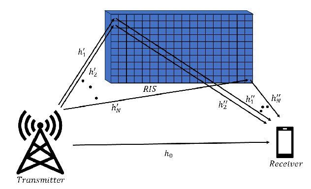
This paper considers that a transmitter communicates with a receiver as shown in Fig. 1. There is also a RIS between the transmitter and the receiver. The received signal at the receiver can be written as
| (1) |
where is the received signal, is the transmitted signal, and is the additive white Gaussian noise (AWGN). The channel between the transmitter and the receiver, denoted as , can be expressed as [26]
| (2) |
In (2), is the number of RIS elements, is the direct channel between the transmitter and the receiver, is the channel between the transmitter and the th RIS element, is the reflection coefficient of the th RIS element, is the channel between the th RIS element and the receiver. Since h is a complex number, it will have a magnitude and a phase. In this paper, denotes the phase of the complex number .
The overall channel from the transmitter to the receiver through the th RIS element can be expressed as
| (3) |
It is also useful to define the cascaded channel coefficient for the th RIS element as
| (4) |
The channel capacity from the transmitter to the receiver can be calculated as
| (5) |
in which is the transmitted signal bandwidth, is the transmitted signal power, is the noise power spectral density, and is the signal-to-noise ratio (SNR).
II-B Practical RIS Reflection Coefficient Model
In general, the reflection coefficient of the th RIS element, denoted as , is defined by two parameters, the amplitude () and the phase shift (). In other words,
| (6) |
In an ideal setup, the amplitude and the phase shift are independent and can take any possible value in a particular range
| (7) |
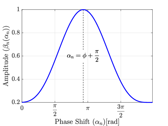
However, the ideal setup is not valid for practical RIS. According to [36], for any circuit implementation of RIS, and are not independent, and the relation between them can be expressed as
| (8) |
where , , and are all non-negative constants. Such a practical model motivated us to consider the phase shift and the amplitude to be coupled rather than independent for our system model. For better illustration, Fig. 2 demonstrates an example for the relationship between and .111According to [36], we use , , and in the example in Fig. 2.
Moreover, assuming a continuous adjustment for the phase shift is infeasible in practical setups. A better and more realistic assumption would be to consider a finite number of discrete choices of phase shift [31]. Therefore, in our setup, for each RIS element, say the th element, is chosen from a configuration set, i.e., a finite set of choices:
| (9) |
in which amplitude and phase shift are constants and satisfy (8) for .
III Optimal Solution for Capacity Maximization
For a system with a given configuration set as shown in (9), our goal is to maximize the capacity for each channel realization of the system by finding the optimal reflection coefficients of the RIS elements. As seen in (5), should be maximized to get the maximal capacity. Therefore, should be chosen in a way that the summation in (2) has the largest possible magnitude. The capacity maximization problem for any given channel realization of the system (i.e., given ), therefore, can be formulated as:
| (10) | ||||
| s.t. |
We will optimize the problem in (10) in two steps. Consider as the optimal reflection coefficient for the th RIS element and as the resulting optimal channel between the transmitter and the receiver. First, assuming (i.e., the phase of ) is known, we will develop a method for determining for all elements. We will discuss this step in detail in Section III-A.
In practice, is not known at the beginning. Thus, in the next step, we have to go through all possibilities of and find the one with the largest . This may seem an impossible task since there will be infinite possibilities for . However, we will prove that by going through just a finite number of possibilities for , we will be able to find the optimal solution. Sections III-B III-E give details of our method and related analysis, insights, and proofs.
III-A Determining by Assuming is Known
Assume is known. Consider the th RIS element. According to (9), there will be choices for . Thus, there will also be choices for (expression of is given in (3)), i.e., , with
| (11) |
for .
Let us define as:
| (12) |
If we view complex numbers and as vectors in a complex plane, then is actually the real inner product of vector and vector .
We have the following theorem.
Theorem 1.
If is the maximum among , then the optimal reflection coefficient of the th RIS element, denoted as , is .
Proof.
Please refer to Appendix A.
∎
According to Theorem 1, among the choices for of the th RIS element, all we have to do is to find the one that has the largest for .
Also, according to (11), we have:
| (13) |
Using (13), the right-hand side of (12) can now be updated as:
| (14) |
in which (from (11)).
As seen in (14), and are the same for all the members of . Thus, finding the maximum would be equivalent to finding the largest . So if is known, we can determine the optimal reflection coefficient for each RIS element (say the th RIS element) by finding the with the largest . From here on, we refer to the largest as and the corresponding as .
III-B Converting Infinite Possibilities of to a Finite Number of Possibilities
In Section III-A, we find the optimal reflection coefficient for each RIS element with given known . However, in reality, is unknown at the beginning. One method is to go through all possibilities of to find the best one. Since there are infinite possibilities for , this method will not be feasible. But as we will soon show, there is a way to go through a finite number of possibilities for and still be able to find the global optimal solution. This is possible because keep unchanged over a range of .
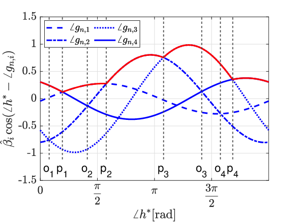
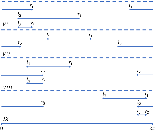
To get a better picture, Fig. 3 shows an example for the th RIS element. In this example, there are choices for , where the four choices are selected randomly from the curve in Fig. 2. The resulting in this example are 1.7279, 3.0369, 4.0841, 5.6549 rad, respectively. Recall that we should find the largest one among , . Fig. 3 shows how the four curves () change with . For presentation brevity, we call curve as “curve ” in the legend of Fig. 3 and in the following discussion.
According to Section III-A, in Fig. 3 we are looking for the maximal of the four curves () at each value. The maximal of the four curves is the red curve shown in Fig. 3. In Fig. 3, are values of the intersections of the curves. From Fig. 3, when changes from 0 to , curve is always above the other three curves, and thus, remains unchanged (keeps as ). Similarly, when changes within , , , or , remains as , , , or , respectively.
We refer to the interval of (within ) over which one curve stays above all other curves as the active interval of the curve. Thus, in Fig. 3, the active intervals of curves , , and are , , and , respectively, and the active interval of curve is the union of two sub-intervals at the two sides of : . For presentation simplicity, we represent as . As a summary, we have the following definition for an interval of written as where :
-
•
if , then the interval is a continuous interval from to (e.g., the active intervals of curves , , and );
-
•
if , then the interval is the union of two continuous sub-intervals located at the two sides of , which is (e.g., the active interval of ).
In either case, and are called the left and right boundary of interval .
We call the right boundary ( value) of the active interval of a curve as the active intersection of the curve. For example, is the active intersection for curve , and is the active intersection for curve .
Since (and ) remains unchanged if is within an active interval, we do not need to go through the infinite possibilities of . As long as we determine the active intervals, we can get (and ) in each active interval. For example, for Fig. 3, when is within active interval , , , and , is , , , and , respectively.
III-C Determining Active Intervals of One RIS Element
For each RIS element, say the th element, its has choices: , corresponding to curves called curve () over , similar to the curves in Fig. 3. Recall that .
To find the intersections ( values) of curves and , we need to solve the following equation:
| (15) | ||||
From (15), the two curves intersect at two points in the range of : one at and the other at . Note that the two intersections are radians apart.
For the curves of the th RIS element, the total number of intersections will be . Among all the intersections, only the active intersections matter to us. For example, as seen in Fig. 3, intersections and are not active and therefore not of any importance to our optimization goal.
Let us consider the intersections on a single curve. It has two intersections with any of the other curves. Thus, the total number of intersections on a single curve will be . For example, in Fig. 3, since there are 4 curves in total, each curve has intersections on it.
Considering the intersections on each curve, there will be an interval between every two consecutive intersections, making the total number of intervals on each curve being .222The intersections partition range of into intervals. As aforementioned, the union of the interval from to the left-most intersection and the interval from the right-most intersection to is viewed as a single interval. Note that by an “interval”, we mean an interval of .
In the following theorem, we prove that the considered curve can have at most one active interval among all intervals.
Theorem 2.
For each curve of the th RIS element, at most one of the intervals is active.
Proof.
Please refer to Appendix B.
∎
According to Theorem 2, each curve will have at most one active interval. Recall that there are curves associated with each RIS element. Therefore, there will be at most active intervals for each RIS element. This means that the number of active intersections for each RIS element can at most be . Next, we will develop a method for finding the active intersections of each RIS element, say the th RIS element.
For the th RIS element, it has curves. Suppose is the interval at which curve is above curve , i.e., . can be determined with the help of the intersection points of the two curves as discussed at the beginning of Section III-C. For the example in Fig. 3, we have and .
For curve , its active interval denoted as can be determined as
| (16) |
Note that refers to the common range of intervals. The following function helps us find the common range of two intervals.
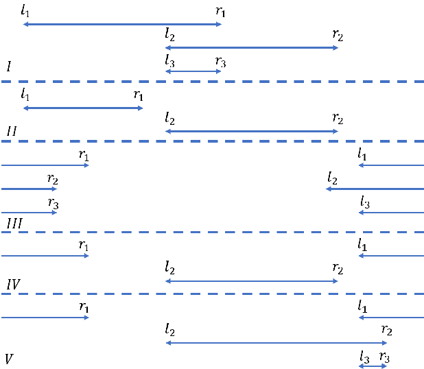
Common range calculator (CRC): The CRC function takes two intervals and as input intervals, and gets interval as the common range (CR) of the two input intervals. Here the intervals follow the interval definition in Section III-B, and ‘’ and ‘’ mean the left and right boundary of an interval, respectively. Table I summarizes the CRC calculation results for different cases (in which “No CR” means that the two input intervals do not have a range in common), and Fig. 4 provides a demonstration for each case in Table I.
By using the CRC, we can get , i.e., the active intervals of the curves associated with the th RIS element. Based on the active intervals, we can get the active intersections for the active intervals of the th RIS element.
| Index | Case | ||
| No CR | No CR | ||
| No CR | No CR | ||
| No CR | No CR | ||
III-D Determining the Active Intersections of All Elements
After we get the active intersections for the th RIS element, we can quickly get active intersections for any other RIS element, say the th RIS element, as follows.
Since , we have:
| (17) |
So is the th curve of the th RIS element. If we shift this curve to the left by (i.e., we replace with ), we will get curve = = , which is the th curve of the th RIS element. Therefore, if we shift all the curves of the th RIS element by the constant value of , we will end up with the curves of the th RIS element. As a result, the active intersections of the th RIS element would be the active intersections of the th RIS element shifted by . Thus, simply by shifting, we can calculate the active intersections of the rest of the elements.
III-E Determining Overall Optimal Reflection Coefficients
In Section III-D, we have determined the active intersections for all RIS elements. Since each RIS element has at most active intervals and at most active intersections, there will be at most active intersections in total for all RIS elements. The active intersections partition the range of into at most regions. As discussed in Section III-B, when is within one region, remain unchanged. Thus, we only need to go through at most regions of , find and the corresponding channel capacity when is within each region, and pick up the largest channel capacity and select the in the corresponding region as the overall optimal reflection coefficients for the RIS elements. Since we only need to go through at most regions, our method has a complexity linear with and .
IV Configuration Set Selection
In Section III, we have demonstrated how capacity maximization is performed for any channel realization of the system, assuming a given configuration set, i.e., a set of reflection coefficient choices as shown in (9). In this section, our target is to select the optimal configuration set for the considered system such that the expected capacity is maximized.
In the literature, most of the works assume that the phase shifts of the reflection coefficient choices are evenly spaced [29, 30, 31, 32], i.e., . This setting is reasonable when the amplitude and phase shift of a reflection coefficient can be adjusted independently. However, in our system, the amplitude and phase shift are coupled. Thus, in general, a configuration set with evenly spaced phase shifts of the reflection coefficients does not guarantee optimality.
Since amplitude is a function of phase shift, selecting a configuration set is equivalent to selecting phase shifts: . As we can see in Fig. 2, the phase shifts can be any value within . Thus, theoretically, there are an infinite number of possible configuration sets for the system. To make the setup feasible, we consider selecting phase shifts from a large number, denoted as (), of evenly spaced phase shifts over the range . We have the following notation definitions.
-
•
Denote the set of evenly spaced phase shifts as .
-
•
Define a -size subset of as a subset of with the size of the subset being .
-
•
Define as the set of all -size subsets of .
So we have . Therefore, our objective is to select a -size subset of , denoted , such that the expected capacity of the system is maximized. In the sequel, is also called a configuration set of the system.
The configuration set selection problem can be formulated as
| (18) |
where is the maximal capacity over a channel realization of the system with the configuration set , and the expectation is over all channel realizations of the system.
An intuitive method to solve the configuration set selection problem in (18) is to use Monte Carlo simulations, referred to as Monte Carlo Simulation based (MCSB) method. In this method, we go through all options of . For each option, we simulate a large number, denoted , of channel realizations of the system. For each realization, we calculate the maximum capacity using the method described in Section III. Then for the option, we average the achievable maximal capacity associated over all channel realizations. In the end, we select the option with the largest average achievable capacity.
In MCSB method, a large number of channel realizations are required for each of the options of . Moreover, at each channel realization, the capacity maximization method in Section III must be applied which has a complexity of . Thus, the total complexity of the MCSB method is , which is time-consuming. Next, we will propose a much faster method that does not require any Monte Carlo simulations and has insights.
IV-A Integral Maximization Based (IMB) Configuration Set Selection
Before we present our method, we introduce two functions and as follows.
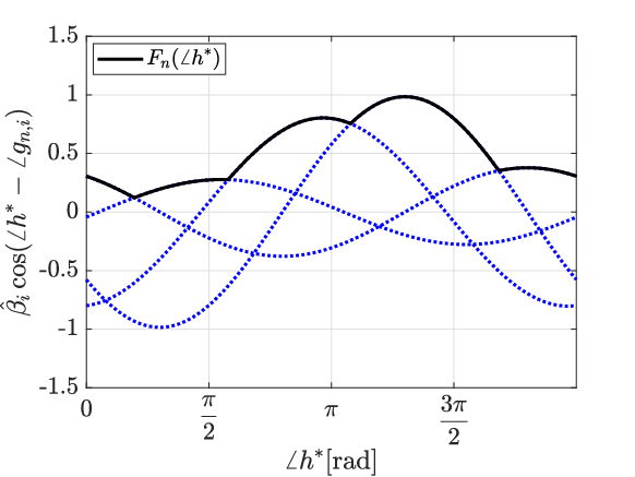
In Section III, for the th RIS element, we have shown that we should get the maximal of curves , for any . Accordingly, for the th RIS element, we can define as the maximal of the curves for a given value, as
| (19) |
Fig. 5 shows an example of function with . For an RIS with elements, we have different functions: .
Also define function as
| (20) |
Accordingly, we have
| (21) | ||||
Equation (21) means that if we shift curve , for any , to the left by , then we can get curve . From (21), we also have
| (22) |
Next, we introduce our method for configuration set selection.
Consider (the maximal capacity over a channel realization of the system with the configuration set ). For presentation simplicity, we omit subscript ‘’ and write as in the sequel. For , its expectation over channel realizations is expressed as
| (23) | ||||
in which (a very large number) is the number of channel realizations, and means the optimal overall channel from the transmitter to the receiver in the th realization.
The term in (23) is expressed as:
| (24) | ||||
We assume are approximately the same and are equal to constant .333This is a common assumption when RIS is at the far field of the transmitter and the receiver [26]. Also assuming a weak direct path (), can be further expressed from (24) as
| (25) | ||||
Here step (i) is from (22), and step (ii) is to use the integral to replace Riemann sum. As we can see in (25), is proportional to .
Theorem 3.
is always non negative.
According to (23), (25) we have
| (26) | ||||
in which the last equality comes from the fact that is always non-negative (Theorem 3). According to (26), since is an increasing function, maximizing would be equivalent to maximizing , which is a major insight of our method.
So in our method, when we go through all options of , we no longer need to consider Monte Carlo simulations with a large number of channel realizations. For each option, we only need to compute . The option corresponding to the largest will be considered as the optimal configuration set. Since our method finds the maximal integral of , we call our method Integral Maximization Based (IMB) method.
IV-B Search Space Compression (SSC)
In Section IV-A, given (a set of evenly distributed phase shifts over range )), the proposed IMB method selects the best option of among all options. Next, we show how we should pick up the evenly distributed phase shifts over range .
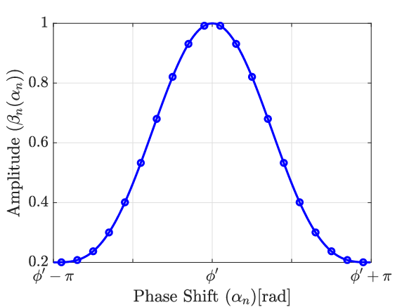
Picking up evenly distributed phase shifts over range is actually picking up points on the curve in Fig. 2 over phase shift range . Note that in Fig. 2, the curve is symmetric over line (in which with being a constant) if we view the range of as . Thus, we select to pick up points on the curve over phase shift range , as shown in Fig. 6.444Picking up points over phase shift range is equivalent to picking up points over phase shift range . The curve in Fig. 6 is perfectly symmetric over line .
To pick up points on the symmetric curve in Fig. 6, intuitively the points should be symmetric over line . Accordingly, should be expressed as
| (27) |
Fig. 6 also shows an example of how points can be chosen on the curve.
Recall that for a given , our proposed IMB method should go through all options of . Next, we show that for given in (27), some options of yield the same , and thus, we actually do not have to go through all options.
Consider an option from (recalling that is the set of all -size subsets of ). In , we have phase shifts, which are corresponding to points (among the points) on the curve in Fig. 6. For presentation simplicity, we denote as , in which are the reflection coefficient choices of option (which are also points among the points on the curve in Fig. 6). Now consider another option from , denoted , in which point and point () are symmetric over the symmetric line in Fig. 6. In other words, and have the same amplitude but their phases are mirrored over the symmetric line, i.e., . We say option and option are mirrored option to each other. For the two options, the function is denoted as and , respectively. We have
| (28) | ||||
Then we have
| (29) | ||||
Here in step (iii) we replace by , in step (iv) we replace with , and in step (v) we use the fact that is a periodical function with period .
Equation (29) shows that for the two options and , the integral of and are the same. Thus, we only need to check one of the two options. We call this as Search Space Compression (SSC).
-
•
If is an even number, then among all options of , some options are identical to their mirrored options, and the number of such options is . Thus, the total number of options of that need to be checked is , which is approximately since is large.
-
•
If is an odd number, there will be two cases. When is even, each option is different from its mirrored option, and thus, the total number of options of that need to be checked is . When is odd, the number of options of that are identical to their mirrors is . Thus, the total number of options of that need to be checked will be , which is approximately since is large.
Therefore, by the SSC method, the number of options that should be checked is cut approximately by half.
V Numerical Results
In this section, we will evaluate the performance of our proposed methods for capacity maximization and configuration set selection. In the following simulations, the parameters are set according to Table II unless specified otherwise.
V-A Capacity Maximization
We simulate our capacity maximization method in Section III as well as three benchmark methods as follows.
-
•
Exhaustive search method: we go through all possibilities of {} to find the optimal phases.
-
•
Closest point projection (CPP): CPP is a heuristic algorithm used in [26]. The idea of this algorithm is to align all RIS channels toward the direct channel as much as possible. In other words, would be the one that maximizes .
-
•
Improved CPP: In the CPP method in [26], phase shift and amplitude of a reflection coefficient can be independently adjusted. Since we consider and to be coupled, we make some changes to the original CPP method by using our result in Theorem 1 as follows. Instead of aligning all RIS channels toward the direct channel, we maximize the inner product of each RIS channel with the direct channel. This means we are maximizing the projection of all RIS channels on the direct channel. Thus, will now be the one that maximizes . This method is called improved CPP.
| Parameter | Value | Parameter | Value |
|---|---|---|---|
| MHz | dB | ||
| dB | Uniform | ||
| dB |
In our simulations, the reflection coefficient of each RIS element is chosen from choices as shown in (9), while the choices have evenly distributed phase shifts, i.e., .
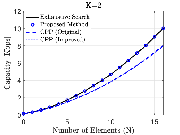
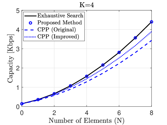
Fig. 7 shows how capacity changes with the number of elements for different algorithms with . According to (2) and (5), we expect the capacity to be an increasing function of , which is verified by the four curves in Fig. 7. As seen in Fig. 7, for all values of , our proposed method yields the same capacity as the exhaustive search method, which means that our method can achieve optimality with linear complexity. The original CPP and the improved CPP have the same performance. This happens because is set to two, hence and are radians apart. Thus, and will have opposite signs. As a result, the amplitude no longer matters.
In Fig. 8, is set to 4. Our method and the exhaustive search method still have the optimal performance. By using our result in Theorem 1, improved CPP outperforms the original CPP but still yields a suboptimal solution.
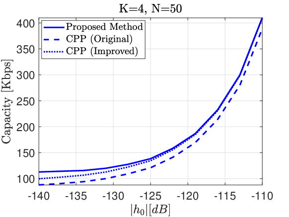
In Fig. 9, we examine how the strength of the direct channel affects the performance of the mentioned methods. According to (2), (5), the capacity is expected to be an increasing function of . At , the proposed method has a noticeable advantage over the improved CPP. But as increases, the gap between the two diminishes. The reason is that when the direct channel becomes stronger, will become the dominant term in (2), and thus, its phase and amplitude greatly affect . As a result, will become an appropriate approximation for . In other words, the improved CPP would be a proper estimate for our proposed method when the direct channel is strong.
V-B Configuration Set Selection
Next, we use simulations to evaluate the performance of our configuration set selection method IMB as well as the IMB method enhanced with the SSC method (denoted as “IMB+SSC”). As a comparison, we also simulate two other methods: 1) the MCSB method with channel realizations for each simulation setup, and 2) the evenly distributed configuration set selection method in which the phase shifts of the reflection coefficients in the configuration set are evenly distributed (i.e., ).
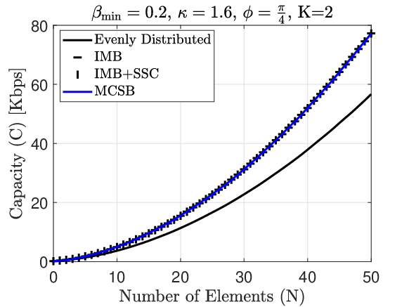
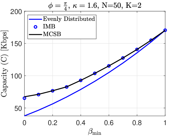
Fig. 10 demonstrates the performance of different methods used for configuration set selection. As the MCSB method uses Monte Carlo Simulations, it can be viewed as the optimal method. As we can see in Fig. 10, MCSB achieves the maximal capacity, while our IMB and IMB+SSC have the same performance with almost negligible difference from the performance of MCSB, which means that our IMB and IMB+SSC achieve an almost-optimal performance, and the SSC method reduces search space without any performance degradation. The evenly distributed configuration set selection method has less capacity than MCSB, IMB, and IMB+SSC.
Since IMB and IMB+SSC have the same capacity performance, we do not show the results of IMB+SSC in Figs. 11-13.
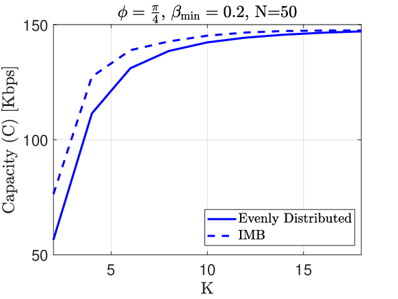
Fig. 11 depicts how capacity changes with in our IMB method and the evenly distributed configuration set selection method. The performance of MCSB method is not shown in this figure, due to the prohibitive simulation time needed for the MCSB method. As we expected, in both IMB and the evenly distributed configuration set selection methods, increasing would provide us with a capacity gain. The gain is large for small values of (e.g. from to ). This suggests that increasing to a large number would be unnecessary and considering small values for (e.g., ) would be sufficient.
Next, we will discuss how the parameters in the reflection coefficient model in (8) influences the performance of different configuration set selection methods.
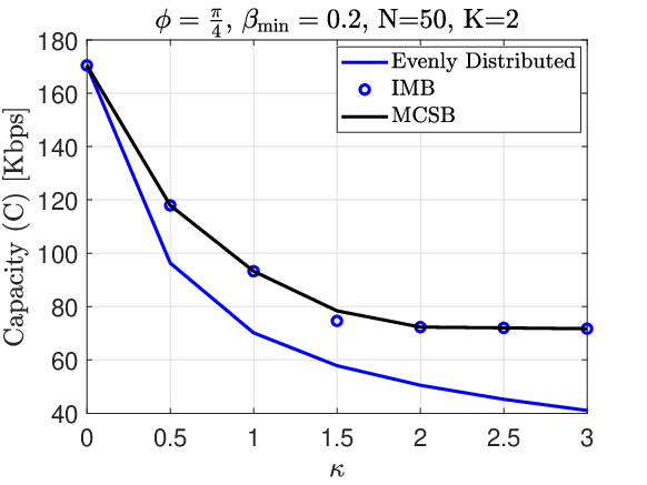
Fig. 12 shows how affects the capacity of the configuration set selection methods. According to (8), represents the amount of loss in an RIS element. High indicates that the element has low loss whereas low implies that the element is quite lossy. Thus, we expect the capacity to be an increasing function of for all methods. When , equation (8) reduces to , which means that the amplitude and phase shift are not coupled anymore, and thus, any set of reflection coefficients whose phase shifts are evenly spaced would be the optimal solution. So all methods yield the same capacity at . It can also be observed that our proposed method (IMB) is most effective when the RIS elements are highly lossy, i.e., when is small.
We can see the effect of of (8) on the performances of the configuration set selection methods in Fig. 13. Similar to , is also an indicator of the degree of loss in an RIS element. In contrast to , the value is proportional to the amount of loss. As a result, we expect the achievable capacity to be a decreasing function of . Similar to Fig. 12, in the lossless scenario (), we have , and thus, all methods achieve the same capacity.
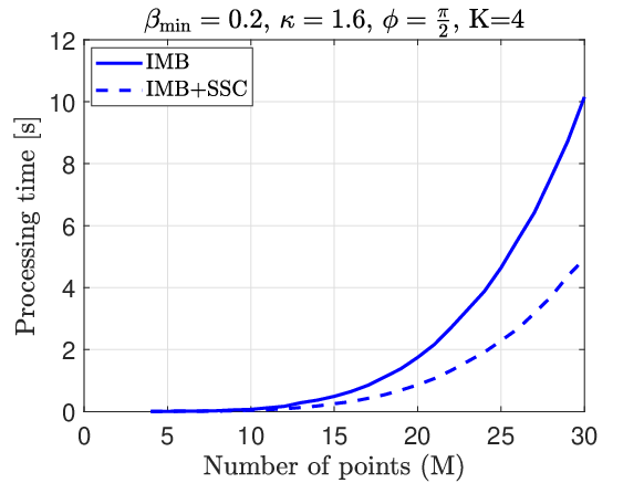
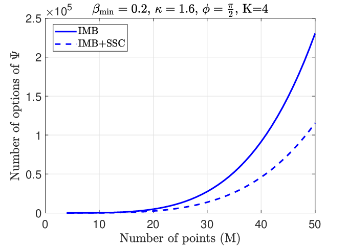
Next, we demonstrate the benefit of IMB+SSC compared to IMB. Fig. 14 demonstrates the processing time for IMB and IMB+SSC. The processing time is defined as the time that a method takes during determining the configuration set. As we can see, the IMB+SSC method is almost twice as fast as the original IMB. Fig. 15 shows the number of options of that each method has to go through. As we expected, when SSC is applied to IMB, the number of searched options gets almost halved resulting in a more compact search space.
VI Conclusion
In this paper, we work on the discrete reflection optimization of RIS elements. In contrast to most works in the literature, we consider a practical setup in which the amplitude and the phase shift of RIS elements are coupled. To maximize the capacity of a system with a given configuration set, we develop an algorithm that yields the global optimal reflection coefficients of RIS elements with linear complexity. We also develop an efficient method called “IMB” that finds the optimal configuration set. Our method is based on our insightful finding that maximizing the average system capacity is approximately equivalent to maximizing the integral . Numerical results show that our capacity maximization method and configuration selection method have apparent gains in terms of channel capacity. In this work, we investigate a single-user setup. However, as discussed in Section I, techniques such as RIS partitioning and/or distributed RIS deployment can help us straightforwardly extend our methods to multi-user setups.
Appendix A Proof of Theorem 1
We use proof by contradiction. Assume . Let us consider . From the optimal reflection coefficients of all RIS elements that achieve , if we replace the reflection coefficient of the th RIS element with , then the overall channel from the transmitter to the receiver is denoted as . Since we assume that is not optimal, should be smaller than . We will have:
| (30) | ||||
| (step (i) is due to additivity property of inner product) | ||||
is a non-negative number. Since is the maximum among , is also a non-negative number. Thus, we have reached a contradiction in the last line of (30). The proof is now complete.
Appendix B Proof of Theorem 2
Consider curve . Assume the interval between two consecutive intersections and on the curve555Here and are values of the two intersections. is an active interval. Assume is the intersection in common between curve and curve . The interval from to is assumed to be active for curve . Thus, we have . At the beginning of Section III-C, we have proved that the intersections in common between each pair of curves are radians apart. Therefore, we can say .666Recall that each interval is defined within in Section III-B. Here interval actually means . We use for presentation simplicity. In general, when we write an interval as , it actually means . We will have:
| (31) | ||||
According to (31), cannot be the maximum curve (i.e., the curve above all other curves) . Now, assume is the intersection in common between and . We have . Since the interval from to is active for curve , we have . We will have:
| (32) | ||||
According to (32), cannot be the maximum curve . Since covers the whole range, there will be no active interval outside for curve . This completes the proof.
References
- [1] Q. Wu and R. Zhang, “Intelligent reflecting surface enhanced wireless network via joint active and passive beamforming,” IEEE Trans. Wireless Commun., vol. 18, no. 11, pp. 5394–5409, Nov. 2019.
- [2] H. Shen, W. Xu, S. Gong, Z. He, and C. Zhao, “Secrecy rate maximization for intelligent reflecting surface assisted multi-antenna communications,” IEEE Commun. Lett., vol. 23, no. 9, pp. 1488–1492, Sep. 2019.
- [3] X. Tan, Z. Sun, D. Koutsonikolas, and J. M. Jornet, “Enabling indoor mobile millimeter-wave networks based on smart reflect-arrays,” Proc. IEEE INFOCOM 2018, pp. 1–6.
- [4] Y. Cheng, K. H. Li, Y. Liu, K. C. Teh, and H. V. Poor, “Downlink and uplink intelligent reflecting surface aided networks: NOMA and OMA,” IEEE Trans. Wireless Commun., vol. 20, no. 6, pp. 3988–4000, Jun. 2021.
- [5] R. Li, B. Guo, M. Tao, Y.-F. Liu, and W. Yu, “Joint design of hybrid beamforming and reflection coefficients in RIS-aided mmWave MIMO systems,” IEEE Trans. Commun., vol. 70, no. 4, pp. 2404–2416, Apr. 2022.
- [6] N. K. Kundu, Z. Li, J. Rao, S. Shen, M. R. McKay, and R. Murch, “Optimal grouping strategy for reconfigurable intelligent surface assisted wireless communications,” IEEE Wireless Commun. Lett., vol. 11, no. 5, pp. 1082–1086, May 2022.
- [7] E. Björnson, Ö. Özdogan, and E. G. Larsson, “Intelligent reflecting surface versus decode-and-forward: How large surfaces are needed to beat relaying?” IEEE Wireless Commun. Lett., vol. 9, no. 2, pp. 244–248, Feb. 2020.
- [8] S. Liu, R. Liu, M. Li, Y. Liu, and Q. Liu, “Joint BS-RIS-user association and beamforming design for RIS-assisted cellular networks,” IEEE Trans. Veh. Technol., vol. 72, no. 5, pp. 6113–6128, May 2023.
- [9] Q. Wu and R. Zhang, “Intelligent reflecting surface enhanced wireless network: Joint active and passive beamforming design,” in Proc. IEEE Global Commun. Conf. (GLOBECOM), Dec. 2018, pp. 1–6.
- [10] S. Zhang and R. Zhang, “Capacity characterization for intelligent reflecting surface aided MIMO communication,” IEEE J. Sel. Areas Commun., vol. 38, no. 8, pp. 1823–1838, Aug. 2020.
- [11] S. Zhang and R. Zhang, “On the capacity of intelligent reflecting surface aided MIMO communication,” in Proc. IEEE Int. Symp. Inf. Theory (ISIT), Jun. 2020, pp. 2977–2982.
- [12] B. Zheng, Q. Wu, and R. Zhang, “Intelligent reflecting surface-assisted multiple access with user pairing: NOMA or OMA?” IEEE Commun. Lett., vol. 24, no. 4, pp. 753–757, Apr. 2020.
- [13] H. Li, W. Cai, Y. Liu, M. Li, Q. Liu, and Q. Wu, “Intelligent reflecting surface enhanced wideband MIMO-OFDM communications: From practical model to reflection optimization,” IEEE Trans. Commun., vol. 69, no. 7, pp. 4807–4820, Jul. 2021.
- [14] Y. Tang, G. Ma, H. Xie, J. Xu, and X. Han, “Joint transmit and reflective beamforming design for IRS-assisted multiuser MISO SWIPT systems,” in Proc. IEEE Int. Conf. Commun. (ICC), Jun. 2020, pp. 1–6.
- [15] Q. Sun et al., “Joint receive and passive Beamforming optimization for RIS-assisted uplink RSMA systems,” IEEE Wireless Commun. Lett., vol. 12, no. 7, pp. 1204–1208, Jul. 2023.
- [16] P. P. Perera, V. G. Warnasooriya, D. Kudathanthirige, and H. A. Suraweera, “Sum rate maximization in STAR-RIS assisted full-duplex communication systems,” in Proc. IEEE Int. Conf. Commun. (ICC), May 2022, pp. 3281–3286.
- [17] Z. Li, W. Chen, Q. Wu, K. Wang, and J. Li, “Joint beamforming design and power splitting optimization in IRS-assisted SWIPT NOMA networks,” IEEE Trans. Wireless Commun., vol. 21, no. 3, pp. 2019–2033, Mar. 2022.
- [18] C. Huang, A. Zappone, G. C. Alexandropoulos, M. Debbah, and C. Yuen, “Reconfigurable intelligent surfaces for energy efficiency in wireless communication,” IEEE Trans. Wireless Commun., vol. 18, no. 8, pp. 4157–4170, Aug. 2019.
- [19] G. Yang, X. Xu, and Y.-C. Liang, “Intelligent reflecting surface assisted non-orthogonal multiple access,” in Proc. IEEE Wireless Commun. Netw. Conf. (WCNC), May 2020, pp. 1–6.
- [20] Q.-U.-A. Nadeem, A. Kammoun, A. Chaaban, M. Debbah, adn M.-S. Alouini “Asymptotic max–min SINR analysis of reconfigurable intelligent surface assisted MISO systems,” IEEE Trans. Wireless Commun., vol. 19, no. 12, pp. 7748–7764, Dec. 2020.
- [21] M. Makin, S. Arzykulov, A. Celik, A. M. Eltawil, and G. Nauryzbayev, “Optimal RIS Partitioning and Power Control for Bidirectional NOMA Networks,” IEEE Trans. Wireless Commun., vol. 23, no. 4, pp. 3175–3189, Apr. 2024.
- [22] S. Zhang and R. Zhang, “Intelligent reflecting surface aided multi-user communication: Capacity region and deployment strategy,” IEEE Trans. Commun., vol. 69, no. 9, pp. 5790–5806, Sep. 2021.
- [23] A. Khaleel and E. Basar, “A novel NOMA solution with RIS partitioning,” IEEE J. Sel. Topics Signal Process., vol. 16, no. 1, pp. 70–81, Jan. 2022.
- [24] J. Mao and A. Yener, “Iterative power control for wireless networks with distributed reconfigurable intelligent surfaces,” in Proc. IEEE Global Commun. Conf. (GLOBECOM), 2022, pp. 3290-3295.
- [25] Q. Wu, S. Zhang, B. Zheng, C. You, and R. Zhang, “Intelligent reflecting surface-aided wireless communications: A tutorial,” IEEE Trans. Commun., vol. 69, no. 5, pp. 3313–3351, May 2021.
- [26] E. Björnson, H. Wymeersch, B. Matthiesen, P. Popovski, L. Sanguinetti, and E. de Carvalho, “Reconfigurable intelligent surfaces: A signal processing perspective with wireless applications,” IEEE Signal Process. Mag., vol. 39, no. 2, pp. 135–158, Mar. 2022.
- [27] R. Fara, P. Ratajczak, D.-T. Phan-Huy, A. Ourir,M. Di Renzo, and J. de Rosny, “A prototype of reconfigurable intelligent surface with continuous control of the reflection phase,” IEEE Wireless Communications, vol. 29, no. 1, pp. 70–77, Feb. 2022.
- [28] C. Pan et al., “An overview of signal processing techniques for RIS/IRSaided wireless systems,” IEEE J. Sel. Topics Signal Process., vol. 16, no. 5, pp. 883–917, Aug. 2022.
- [29] Y. Liu et al., “Reconfigurable intelligent surfaces: Principles and opportunities,” IEEE Commun. Surveys Tuts., vol. 23, no. 3, pp. 1546–1577, 3rd Quart., 2021.
- [30] Q. Wu and R. Zhang, “Beamforming optimization for intelligent reflecting surface with discrete phase shifts,” in Proc. IEEE ICASSP, May 2019, pp. 7830–7833.
- [31] Q. Wu and R. Zhang, “Beamforming optimization for wireless network aided by intelligent reflecting surface with discrete phase shifts,” IEEE Trans. Commun., vol. 68, no. 3, pp. 1838–1851, Mar. 2020.
- [32] S. Ren, K. Shen, X. Li, X. Chen, and Z.-Q. Luo, “A linear time algorithm for the optimal discrete IRS beamforming,” IEEE Wireless Commun. Lett., vol. 12, no. 3, pp. 496–500, Mar. 2023.
- [33] L. Dai et al., “Reconfigurable intelligent surface-based wireless communications: Antenna design, prototyping, and experimental results,” IEEE Access, vol. 8, pp. 45913–45923, 2020.
- [34] S. Hashemi, H. Jiang and M. Ardakani, “Optimal configuration of reconfigurable intelligent surfaces with arbitrary discrete phase shifts,” IEEE Trans. Commun., early access, Jul. 2024, doi: 10.1109/TCOMM.2024.3422220.
- [35] H. Zhang et al., “Intelligent omni-surfaces for full-dimensional wireless communications: Principles, technology, and implementation,” IEEE Commun. Mag., vol. 60, no. 2, pp. 39–45, Feb. 2022.
- [36] S. Abeywickrama, R. Zhang, Q. Wu, and C. Yuen “Intelligent reflecting surface: practical phase shift model and beamforming optimization,” IEEE Trans. Commun., vol. 68, no. 9, pp. 5849–5863, Sep. 2020.
- [37] H. Zhao, M. Peng, Y. Ni, L. Li and M. Zhu, “Joint beamforming and reflection design for RIS assisted bistatic backscatter networks With practical phase shift and amplitude response,” IEEE Commun. Lett., vol. 28, no. 6, pp. 1362–1366, Jun. 2024.
- [38] Y. Zhang, J. Zhang, M. D. Renzo, H. Xiao, and B. Ai, “Performance analysis of RIS-aided systems with practical phase shift and amplitude response,” IEEE Trans. Veh. Technol., vol. 70, no. 5, pp. 4501–4511, May 2021.