Rise and fall of the X-ray flash 080330: an off-axis jet?
Abstract
Context. X-ray flashes (XRFs) are a class of gamma-ray bursts (GRBs) with the peak energy of the time-integrated spectrum, , typically below 30 keV, whereas classical GRBs have of a few hundreds keV. Apart from and the systematically lower luminosity, the properties of XRFs, such as the duration or the spectral indices, are typical of the classical GRBs. Yet, the nature of XRFs and the differences from that of GRBs are not understood. In addition, there is no consensus on the interpretation of the shallow decay phase observed in most X-ray afterglows of both XRFs and GRBs.
Aims. We examine in detail the case of XRF 080330 discovered by Swift at the redshift of . This burst is representative of the XRF class and exhibits an X-ray shallow decay. The rich and broadband (from NIR to UV) photometric data set we collected across this phase makes it an ideal candidate to test the off-axis jet interpretation proposed to explain both the softness of XRFs and the shallow decay phase.
Methods. We present prompt -ray, early and late NIR/visible/UV and X-ray observations of the XRF 080330. We derive a spectral energy distribution from NIR to X-ray bands across the shallow/plateau phase and we describe the temporal evolution of the multi-wavelength afterglow within the context of the standard afterglow model.
Results. The multi-wavelength evolution of the afterglow is achromatic from s out to s. The energy spectrum from NIR to X-ray is nicely fitted with a simple power-law, , with and negligible rest-frame dust extinction. The light curve can be modelled either by a piecewise power-law or by the combination of a smoothly broken power law with an initial rise up to 600 s, a plateau lasting up to 2 ks, followed by a gradual steepening to a power-law decay index of out to 82 ks. At this point, there appears a bump modelled with a second component, while the corresponding optical energy spectrum, , reddens by .
Conclusions. A single-component jet viewed off-axis explains the light curve of XRF 080330, the late time reddening as due to the reverse shock of an energy injection episode, and its being an XRF. Other possibilities, such as the optical rise marking the pre-deceleration of the fireball within a wind environment, cannot be definitely excluded, but seem somewhat contrived. We rule out the dust decreasing column density swept up by the fireball as the explanation of the rise of the afterglow.
Key Words.:
gamma rays: bursts; X-rays: individual (XRF 080330)1 Introduction
Time-integrated photon spectra of long gamma-ray bursts (GRBs) can be adequately fitted with a smoothly broken power law (Band et al. 1993), whose low-energy and high-energy indices, and , have median values of and , respectively (Preece et al. 2000; Kaneko et al. 2006). The corresponding spectrum peaks at , the so-called peak energy, whose rest frame value is found to correlate with other relevant observed intrinsic properties, such as the isotropic-equivalent radiated -ray energy, (Amati et al. 2002), or its collimation-corrected value, (Ghirlanda et al. 2004). In the BATSE catalogue, the distribution clusters around keV with a keV width (Kaneko et al. 2006).
When observations of GRBs in softer energy bands than BATSE became available thanks to BeppoSAX and HETE-2, a new class of soft GRBs with keV, so named X-ray flashes (XRFs), was soon discovered (Heise et al. 2001; Barraud et al. 2003). GRBs with intermediate softness, called X-ray rich (XRR) bursts, were also observed, with keV keV (Sakamoto et al. 2005). These soft GRBs share the same temporal and spectral properties, aside from the systematically lower , with the classical GRBs both for the prompt (Frontera et al. 2000; Barraud et al. 2003; Amati et al. 2004) and, partially, the afterglow emission (Sakamoto et al. 2005; D’Alessio et al. 2006; Mangano et al. 2007). Moreover, they were found to obey the – correlation (Amati et al. 2007) discovered for classical GRBs, extending it all the way down to values of a few keV and forming a continuum (Sakamoto et al. 2005). Like classical GRBs, also XRFs have been found to be associated with SNe (Campana et al. 2006; Pian et al. 2006) and therefore connected with the collapse of massive stars. The comparison also holds for the cases in which apparently no associated SN was found both for classical GRBs (e.g. Della Valle et al. 2006, Fynbo et al. 2006, Gal-Yam et al. 2006) and for XRFs (Levan et al. 2005).
A number of different models have been proposed in the literature to explain the nature of XRRs and XRFs (e.g., see the review of Zhang 2007): i) standard GRBs viewed well off the axis of the jet, thus explaining the softness as due to a larger viewing angle and a lower Doppler factor (Yamazaki et al. 2002; Granot et al. 2002, 2005); ii) two coaxial jets with different opening angles (wide and narrow), , and viewed at an angle , (Peng et al. 2005); iii) the “dirty fireball” model characterised by a small value of the bulk Lorentz factor due to a relatively high baryon loading of the fireball (Dermer et al. 2000); iv) distribution of high Lorentz factors with low contrast of the colliding shells (Mochkovitch et al. 2004). In the off-axis interpretation, a number of different models of the structure and opening angle of the jet have been proposed (e.g. Granot et al. 2005; Donaghy 2006).
The advent of Swift (Gehrels et al. 2004) has made it possible to collect a large sample of early X-ray afterglow light curves of GRBs. Concerning the XRRs and XRFs, the 15–150 keV energy band of the Swift Burst Alert Telescope (BAT; Barthelmy et al. 2005) and its relatively large effective area still allow to detect them, although those with of a few keV are disfavoured with respect to BeppoSAX and HETE-2 instruments (Sakamoto et al. 2008). Thanks to Swift it is possible to study the early X-ray afterglow properties of these soft events. Like hard GRBs, also XRFs occasionally exhibit X-ray flares (Romano et al. 2006). Sakamoto et al. (2008) analysed a sample of XRFs, XRRs and classical GRBs detected with Swift and found some evidence for an average X-ray afterglow luminosity of XRFs being roughly half that of classical GRBs and some differences between the average X-ray afterglow light curves.
An unexpected discovery of Swift is the shallow decay phase experienced by most of X-ray afterglows between a few up to – s after the trigger time (Tagliaferri et al. 2005; Nousek et al. 2006; Zhang et al. 2006). Several interpretations have been put forward (e.g. see Ghisellini et al. 2009 for a brief review). Among them, some invoke continuous energy injection to the fireball shock front through refreshed shocks (Nousek et al. 2006; Zhang et al. 2006), depending on the progenitor period of activity: a long- or short-lived powering mechanism, either in the form of a prolonged, continuous energy release (), or via discrete shells whose distribution is a steep power-law. For instance, in the cases of GRB 050801 and GRB 070110 a newly born millisecond magnetar was suggested to power the flat decay observed in the optical and X-ray bands (De Pasquale et al. 2007; Troja et al. 2007). Alternatively, geometrical models interpret the shallow decay as the delayed onset of the afterglow observed from viewing angles outside the edge of a jet (Granot et al. 2002; Salmonson 2003; Granot 2005; Eichler & Granot 2006). Other models invoke two-component jets viewed off the axis of the narrow component, also invoked to explain the late time observations of GRB 030329 (Berger et al. 2003). In particular, this model would explain the initial flat decay observed in XRF 030723, dominated by the wide component, followed by a late rebrightening peaking at 16 days and interpreted as due to the deceleration and lateral expansion of the narrow component (Huang et al. 2004; Butler et al. 2005), although alternative explanations for this in terms of a SN have also been proposed (Fynbo et al. 2004; Tominaga et al. 2004).
Other models explain the shallow decay as due to a temporal evolution of the fireball micro-physical parameters (Ioka et al. 2006; Granot et al. 2006); scattering by dust located in the circumburst medium (Shao & Dai 2007); “late prompt” activity of the inner engine, keeping up a prolonged emission of progressively lower power and Lorentz factor shells, which radiate at the same distance as for the prompt emission (Ghisellini et al. 2007, 2009); a dominating reverse shock in the X-ray band propagating through late shells with small Lorentz factors (Genet et al. 2007; Uhm & Beloborodov 2007). Yamazaki (2009) suggests that the plateau and the following standard decay phases are an artifact of the choice of , provided that the engine activity begins before the trigger time by – s.
XRF 080330 was promptly discovered by the Swift-BAT and automatically pointed with the X-Ray Telescope (XRT; Burrows et al. 2005) and the Ultraviolet/Optical Telescope (UVOT; Roming et al. 2005) as shown in Figure 3. In this work we present a detailed analysis of the Swift data, from the prompt -ray emission to the X-ray and optical afterglow and combine it with the large multi-filter data set collected from the ground, encompassing a broad band, from NIR to UV wavelengths, and spanning from one minute out to 3 days post burst. The main properties exhibited by XRF 080330 are the rise of the optical afterglow up to 300 s, followed by a shallow decay also present in the X-ray, after which it gradually steepens, and either a possible late time ( s) brightening (Fig. 5) or a sharp break (Fig. 4). The richness of the multi-wavelength data collected throughout the rise-flat top-steep decay allows us to constrain the broadband energy spectrum of the shallow decay phase as well as its spectral evolution. Moreover, it is possible to constrain the optical flux extinction due to dust along the line of sight and, in particular, near the progenitor. This GRB is a good benchmark for the proposed models of XRFs sources and of their link with the classical GRBs through the common properties, such as the flat decay phase.
The paper is organised as follows: Sects. 2 and 3 report the observations, data reduction and analysis, respectively. We report our multi-wavelength combined analysis in Sect. 4. In Sect. 5 we discuss our results in the light of the models proposed in the literature and Sect. 6 reports our conclusions.
Throughout the paper, times are given relative to the BAT trigger time. The convention is followed, where the spectral index is related to the photon index . We adopted the standard cosmology: km s-1 Mpc-1, , .
All the quoted errors are given at 90% confidence level for one interesting parameter (), unless stated otherwise.
2 Observations
XRF 080330 triggered the Swift-BAT on 2008 March 30 at 03:41:16 UT. The -ray prompt emission in the 15–150 keV energy band consisted of a multiple–peak structure with a duration of about 60 s (Mao et al. 2008a). An uncatalogued, bright and fading X-ray source was promptly identified by XRT. From the initial 100-s finding chart taken with the UVOT telescope in the White filter from 82 s the optical counterpart was initially localised at RA , Dec. (J2000), with an error radius of (1; Mao et al. 2008a). During the observations, the Swift star trackers failed to maintain a proper lock resulting in a drift which affected the observations and accuracy of early reports. We finally refined the position from the UVOT field match to the USNO–B1 catalogue: RA , Dec. (J2000), with an error radius of (1; Mao et al. 2008b), consistent with the position derived from ground telescopes (e.g., PAIRITEL, Bloom & Starr 2008).
The Télescopes à Action Rapide pour les Objets Transitoires (TAROT; Klotz et al. 2008c) began observing at s ( s after the notice) and discovered independently the optical counterpart during the rise with at 300 s (Klotz et al. 2008a). TAROT went on observing until the dawn at ks (Klotz et al. 2008b).
The Rapid Eye Mount111http://www.rem.inaf.it/ (REM; Zerbi et al. 2001) telescope reacted promptly and began observing at 55 s and detected the optical afterglow in band (D’Avanzo et al. 2008). The optical counterpart was promptly detected also by other robotic telescopes, such as ROTSE–IIIb (Schaefer et al. 2008; Yuan et al. 2008), PROMPT (Schubel et al. 2008) and RAPTOR; the latter in particular observed a -s long optical flash of at 60 s contemporaneous with the last -ray pulse (Wren et al. 2008).
The Liverpool Telescope (LT) began observing at 181 s. The optical afterglow was automatically identified by the LT-TRAP GRB pipeline (Guidorzi et al. 2006) with (Gomboc et al. 2008a), thus triggering the multi-colour imaging observing mode in the filters which lasted up to the dawn at ks.
The Faulkes Telescope North (FTN) observations of XRF 080330 were carried out from to hr and again from to hr with deep and filter exposures.
The Gamma-Ray Burst Optical and Near-Infrared Detector (GROND; Greiner et al. 2008) started simultaneous observations in filters of the field of GRB 080330 at minutes and detected the afterglow with and from the first 240-s of effective exposure (Clemens et al. 2008).
A spectrum of XRF 080330 was acquired at minutes with the Nordic Optical Telescope (NOT). The identification of absorption features allowed to measure the redshift, which turned out to be (Malesani et al. 2008). This was soon confirmed by the spectra taken with the Hobby-Eberly Telescope (Cucchiara & Fox 2008).
The Galactic reddening along the line of sight to the GRB is (Schlegel et al. 1998). The corresponding extinction in each filter was estimated through the NASA/IPAC Extragalactic Database extinction calculator222http://nedwww.ipac.caltech.edu/forms/calculator.html: , , , , , , , , , , , , .
3 Data reduction and analysis
3.1 Gamma–ray data
The BAT data were processed with the heasoft package (v.6.4) adopting the ground-refined coordinates provided by the BAT team (Markwardt et al. 2008). The BAT detector quality map was obtained by processing the nearest-in-time enable/disable map of the detectors.
The top panel of Figure 1 shows the 15–150 keV mask-weighted light curve of XRF 080330 as recorded by BAT, expressed as counts per second per fully illuminated detector for an equivalent on-axis source. The solid line displayed in Fig. 1 corresponds to the result of fitting the profile from to s with a combination of four pulses (Markwardt et al. 2008) as modelled by Norris et al. (2005; hereafter N05 model). Table 1 reports the corresponding derived parameters: (peak time), (15–150 keV peak flux), (rise time), (decay time), (pulse width), (pulse asymmetry) and the model fluence in the 15–150 keV band. The goodness of the fit is . Parameter uncertainties were derived by propagation starting from the best-fit parameters and taking into account their covariance. We tried to apply the same analysis to the light curves of the resolved energy channels to investigate temporal lags and, more generally, the dependence of the parameters on energy; however, because of the faintness and softness of the signal, we could not constrain the parameters in a useful way.
| Pulse | Fluence | ||||||
|---|---|---|---|---|---|---|---|
| (s) | ( erg cm-2 s-1) | (s) | (s) | (s) | ( erg cm-2) | ||
| 1 | |||||||
| 2 | |||||||
| 3 | |||||||
| 4 |
In addition, the energy spectra in the 15–150 keV band were extracted using the tool batbinevt. We applied all the required corrections: we updated them through batupdatephakw and generated the detector response matrices using batdrmgen. Then we used batphasyserr in order to account for the BAT systematics as a function of energy. Finally we grouped the energy channels of the spectra by imposing a 3 (or 2- when the S/N was too low) threshold on each grouped channel. We fitted the resulting photon spectra, (ph cm-2s-1keV-1), with a power law with pegged normalisation (pegpwrlw model under xspec v.11.3.2). We extracted several spectra in different time intervals: over , total, spanning the bunch of the first three pulses, the fourth pulse alone and that around the peak, determined on a minimum significance criterion. The results are reported in Table 2. The time-averaged spectral index is with a total fluence of erg cm-2 and a -s peak photon flux of ph cm-2 s-1, in agreement with previous results (Markwardt et al. 2008). The bottom panel of Fig. 1 shows marginal evidence for a soft–to–hard evolution: passes from (first three pulses) to (fourth pulse).
Following Sakamoto et al. (2008), a GRB is classified as an XRR (XRF) depending on whether the fluence ratio is lower (greater) than . The fluence ratio of XRF 080330, , places it among the XRFs, although still compatible with being an XRR burst. Although from BAT data alone we could not measure the peak energy of the time-integrated spectrum, we tried to fit with a smoothed broken power law model (Band et al. 1993) by fixing the low-energy index to -1 (Kaneko et al. 2006), given that and is very likely dominated by the high-energy index . This way we derived the following constraint: keV, in agreement with the upper limit to its rest-frame (intrinsic) value, keV, obtained by Rossi et al. (2008).
Recently, Sakamoto et al. (2009) calibrated a method aimed at estimating from the as measured with BAT, provided that . In the case of XRF 080330, the confidence interval on , , marginally overlaps with the allowed range; however, since is anti-correlated with and the lower limit on lies within the usable range, we can derive an upper limit to from the relation of Sakamoto et al. (2009), which turns out to be keV, in agreement with our previous value. These results are fully consistent with a previous preliminary analysis (Markwardt et al. 2008).
We constrained in the rest-frame 1– keV band using the upper limit on of keV. Following the prescriptions by Amati et al. (2002) and Ghirlanda et al. (2004), we found ergs. Combined with keV, this places XRF 080330 in the – space consistently with the Amati relation (Amati et al. 2002; Amati 2006).

3.2 X–ray data
The XRT data were processed using the heasoft package (v.6.4). We ran the task xrtpipeline (v.0.11.6) applying calibration and standard filtering and screening criteria. Data from 77 to 134 s were acquired in Windowed Timing (WT) mode and the following in Photon Counting (PC) mode due to the faintness of the source. Events with grades 0–2 and 0–12 were selected for the two modes, respectively. XRT observations went on up to s, with a total net exposure time of ks. The XRT analysis was performed in the 0.3–10 keV energy band.
Source photons were extracted from WT mode data in a rectangular region 40 pixels along the image strip (20 pixel wide) centred on the source, whereas the background photons were extracted from an equally-sized region with no sources.
Firstly, we extracted the first orbit PC data from 136 to 331 s, where the point spread function (PSF) of the source looked unaffected by the spacecraft drifting, and extracted the following refined position: RA , Dec. (J2000), with an error radius of arcsec (Mao & Guidorzi 2008). We corrected these data for pile-up by extracting source photons from an annular region centred on the above position and with inner and outer radii of 4 and 30 pixels (1 pixel), respectively. The background was estimated from a three-circle region with a total area of pixel2 away from any source present in the field. Finally, we re-extracted the source photons over the entire first orbit within a larger circular region centred on the same position and with a radius of 40 pixels, to compensate for the drifting. The light curve of the full first orbit data (PC mode) was then corrected so as to match the previous one correctly produced in the 136–331 s sub-interval.
The resulting 0.3–10 keV light curve is shown in Fig. 3 (black empty triangles). It was binned so as to achieve a minimum signal to noise ratio (SNR) of 3. The data taken in following orbits were not enough to provide a significant detection and only a 3 upper limit was obtained.
The X-ray curve can be fitted with a broken power law, with the following parameters: , s, (). The last upper limit clearly requires a further break. We set a lower limit on by connecting the end of first orbit data with the late upper limit under the assumption that the second break occurred at the beginning of the data gap. This turned into (3 confidence). The later the second break time, the steeper the final decay.
We extracted the 0.3–10 keV spectrum in two different time intervals: i) “XRT-WT” interval, from to s (WT mode), corresponding to the initial steep decay; ii) “plateau” interval, from to s (PC mode) corresponding to the following flat decay (or “plateau”) phase. Source and background spectra were extracted from the same regions as the ones used for the light curve for the corresponding time intervals and modes. The ancillary response files were generated using the task xrtmkarf. Spectral channels were grouped so as to have at least 20 counts per bin. Spectral fitting was performed with xspec (v. 11.3.2).
We modelled both spectra with a photoelectrically absorbed power law (model wabszwabspow), adopting the photoelectric cross section by Morrison & McCammon (1983). The first column density was frozen to the weighted average Galactic value along the line of sight to the GRB, cm-2 (Kalberla et al. 2005), while the second rest-frame column density, , was left free to vary. While during the steep decay we found no evidence for significant rest-frame absorption, with a 90% confidence limit of cm-2, in the plateau spectrum we found only marginal evidence for it, cm-2. The spectral index, , varies from to : the significance of this change is . The best-fit parameters are reported in Table 2.
3.3 Near–UV/Visible UVOT data
The Swift UVOT instrument started observing on 2008 March 30 at 03:42:19 UT, 63 s after the BAT trigger, with a -s settling exposure. Since the detectors are powered up during this exposure, the effective exposure time may be less than reported. We checked the brightness in this exposure with later exposures, to confirm that no correction was needed. The first -s finding chart exposure started at 03:42:39 UT in the white filter in event mode followed by a -s exposure in the filter, also in event mode. Due to the loss of lock by the spacecraft star trackers, the attitude information was incorrect. In order to process the data, xselect was used to extract images for short time intervals. The length of the interval was chosen short enough that the drift of the spacecraft was mostly within , and at most , but long enough to get a reasonably accurate measurement. A source region was placed over the position of the source, making checks for consistency with the position of nearby stars, and the magnitudes were determined using the ftool uvotevtlc. In most cases, an aperture with a radius of was used, and three measurements used a slightly larger aperture. No aperture correction was made, since the source shape in those cases was very elongated. The measured magnitudes were converted back to the original count rates, using the UVOT calibration (Poole et al. 2008). These were subsequently converted to fluxes using the method of Poole et al. (2008), but for an incident power-law spectrum with and for a redshift .
3.4 NIR/Visible ground-based data
Robotically triggered observations with the LT began at 181 s leading to the automatic identification by the GRB pipeline LT-TRAP (Guidorzi et al. 2006) of the optical afterglow at the position RA , Dec. (J2000; 1 error radius of arcsec). This is consistent within with the refined UVOT position. The afterglow was seen during the end of the rise with and subsequently decay (Gomboc et al. 2008a). Following two initial sequences of s each in the filter during the detection mode (DM), the multi-colour imaging observing mode (MCIM) in the filters was automatically selected. Observations carried on up to ks.
The FTN observations of XRF 080330 were carried out from to hr and again from to hr with deep and filter exposures as part of the RoboNet 1.0 project333http://www.astro.livjm.ac.uk/RoboNet/ (Gomboc et al. 2006).
Calibration was performed against five non-saturated field stars with preburst SDSS photometry (Cool et al. 2008), by adopting their PSF to adjust the zero point of the single images. Photometry was carried out using the Starlink GAIA software. Magnitudes were converted into flux densities (mJy) following Fukugita et al. (1996). Results are reported in Table LABEL:tab:photom.
Optical -band observations of the afterglow of GRB 080330 were carried out with the REM telescope equipped with the ROSS optical spectrograph/imager on 2008 March 30, starting about 55 seconds after the burst (D’Avanzo et al. 2008). We collected 38 images with typical exposures times of 30, 60 and 120 s, covering a time interval of about hours. Image reduction was carried out by following the standard procedures: subtraction of an averaged bias frame, division by a normalised flat frame. The astrometry was fitted using the USNOB1.0444http://www.nofs.navy.mil/data/fchpix/ catalogue. We grouped our images into 18 bins in order to increase the signal-to-noise ratio (SNR) and performed aperture photometry with the SExtractor package (Bertin & Arnouts 1996) for all the objects in the field. In order to minimise the systematics, we performed differential photometry with respect to a selection of local isolated and non-saturated standard stars.
The calibration of NOT images taken with the filter was performed with respect to the converted magnitudes in the -band of the selected set of stars used for the calibration of LT and GROND images in the SDSS passbands. We transformed the and magnitudes of the calibration stars (Cool et al. 2008) into and magnitude following the filter transformations of Krisciunas et al. (1998).
Hereafter, the magnitudes shown are not corrected for Galactic extinction, whilst fluxes as well as all the best-fit models are. When the models are plotted together with magnitudes, the correction for Galactic extinction is removed from the models.
| Interval | Energy band | Start time | Stop time | Mean flux | /dof | |||
| (keV) | (s) | (s) | ( cm-2) | (erg cm-2 s-1) | ||||
| 15–150 | – | – | ||||||
| Total | 15–150 | – | – | |||||
| Pulses 1–3 | 15–150 | – | – | |||||
| Pulse 4 | 15–150 | – | – | |||||
| Peak | 15–150 | – | – | |||||
| XRT-WT | 0.3–10 | – | ||||||
| Plateau | 0.3–10 | – | ||||||
| SED 2 | opt–X | – | ||||||
| SED 3 | opt–X | – | ||||||
| SED 4 | opt | – | – | |||||
| SED 2 | opt | – | – | |||||
| SED 3 | opt | – | – | |||||
| SED 4 | opt | – | – |
3.5 Spectroscopy
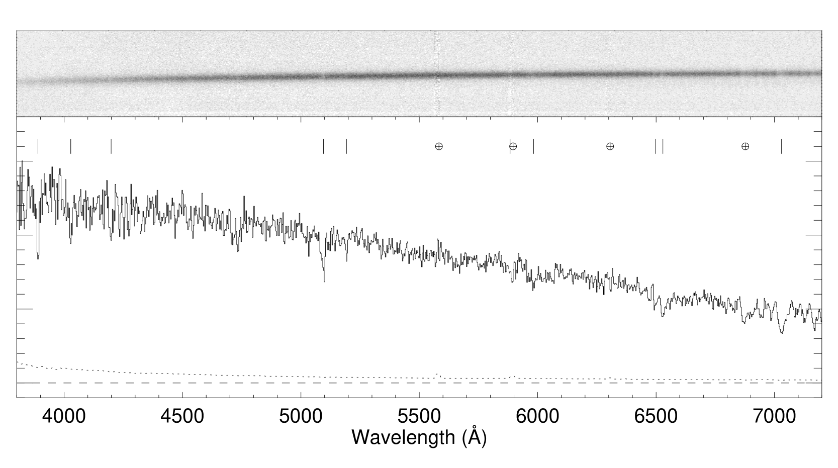
Starting at min we obtained a 1800 s spectrum with a low resolution grism and a 1.3 arcsec wide slit covering the spectral range from about 3500 to 9000 Å at a resolution of 14 Å with the NOT (Fig. 2). The airmass was about 1.8 at the start of the observations. The spectrum was reduced using standard methods for bias subtraction, flat-fielding and wavelength calibration using an Helium-Neon arc spectrum. The rms of the residuals in the wavelength calibration were about 0.3 Å. The spectrum was flux-calibrated using an observation with the same setup of the spectrophotometric standard star HD93521. Table 6 reports the identified lines.
4 Multi-wavelength combined analysis
4.1 Panchromatic light curve
Figure 3 displays the light curves of the prompt emission (15–150 keV) and of the 0.3–10 keV and NIR/visible/UV afterglow derived from our data sets plus some points taken from RAPTOR (Wren et al. 2008). High-energy fluxes (magnitudes) are referred to the right-hand (left-hand) y-axis. First of all, we note that the peak time of the last -ray pulse (Table 1) is contemporaneous with the optical flash detected by RAPTOR, reported at s (Wren et al. 2008).
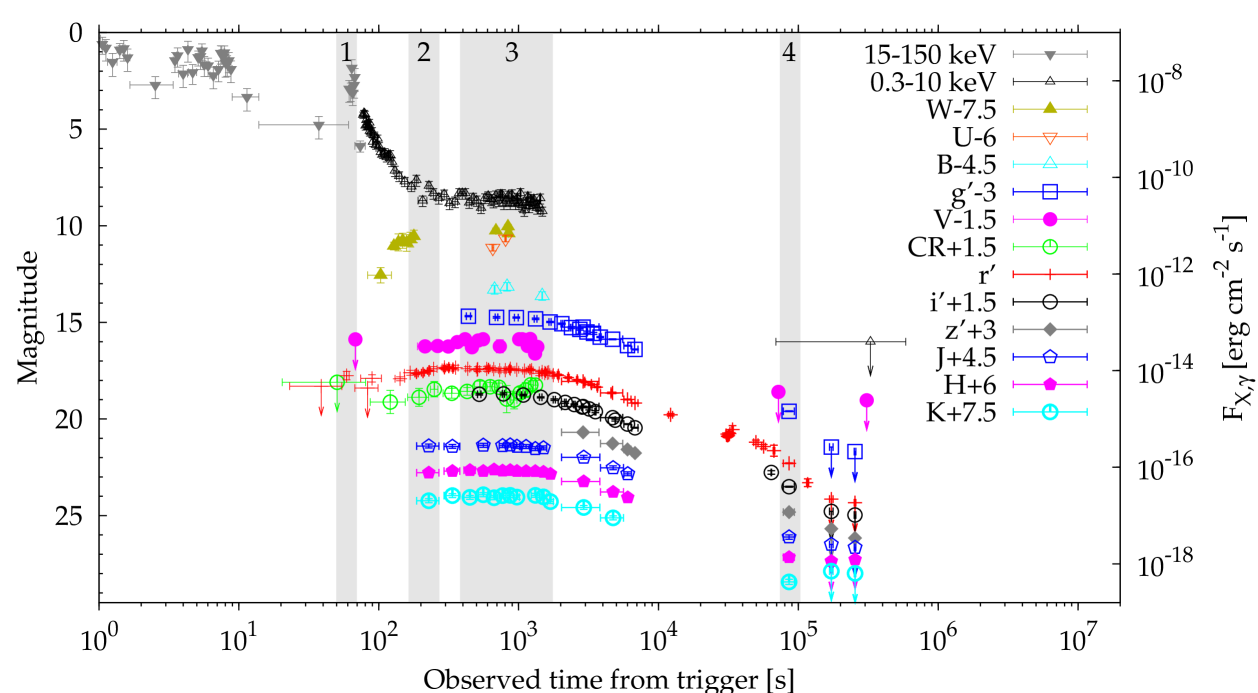
The initial steep decay observed by XRT is a smooth continuation of the last -ray pulse and is thus the tail of the prompt GRB emission, and likely to correspond to its high-latitude emission. Most notably, during the X-ray steep decay the optical flux is seen to rise up to s and finally a simultaneous plateau is reached at both energy bands, lasting up to s, when the X-ray observations stopped. This strongly suggests that the plateau is emission from a region which is physically distinct from that responsible for the prompt emission and its tail (the rapid decay phase).
As discussed in Sect. 4.2, the afterglow does not show evidence for spectral evolution throughout the observations, except for late epochs ( s), when there is evidence for reddening. The achromatic nature of the afterglow light curve allows for a multi-wavelength simultaneous fit of twelve light curves, where only the normalisations are left free to vary independently from each other. We consider all of the available passbands: , , , , , , , , , , and X-ray, respectively. The latter curve is fitted from 300 s onward, so as to exclude the initial steep decay. Hereafter we present two alternative combinations of models, both providing a reasonable description of the flux temporal evolution. In both cases we had to add a 2% systematics to all of the measured uncertainties to account for some residual variability with respect to the models, in order to have acceptable values and correspondingly acceptable parameters’ uncertainties.
4.1.1 Multiple smoothly broken power law
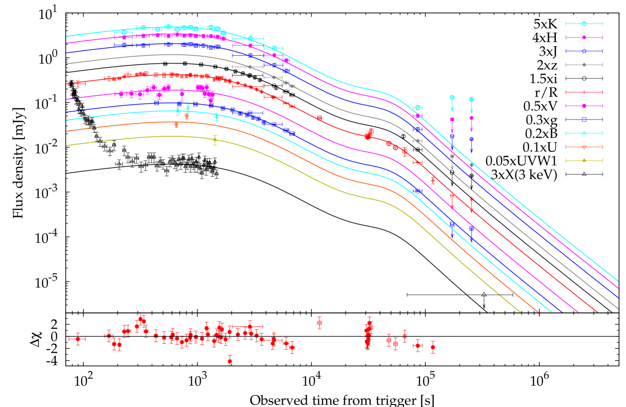
A possible description of the light curves is offered by a multiple broken power law (Fig. 4). This has the advantage of a more straightforward interpretation in terms of the standard fireball evolution model due to synchrotron emission. We started from the parametrisation by Beuermann et al. (1999) and added two more breaks to finally provide a sufficiently detailed description. The fitting function is given by eq. (1).
| (1) |
The free parameters are the normalisation constant (different for each curve), , three break time constants, (), four power-law indices, , the smoothness . Apart from the normalisations, all the curves share the same parameters. Overall, the free parameters and the degrees of freedom (dof) total 20 and 184, respectively.
Equation (1) looks like a piecewise power law only in the following regime: , where each individual term takes over at well separate epochs. The light curve of XRF 080330 fits in this case, as proven by the best-fit results (first line of Table 3) and shown in Fig. 4. The effective break times, , , , i.e. the times at which the model (1) changes the power-law regime, are simply given by , , .
The goodness of the fit in terms of is 212/184, corresponding to a non-rejectable P-value of %. The normalisation constants for the different bands are the following (Jy): , , , , , , , , , , , while the X-ray normalisation, expressed in flux units in the 0.3–10 keV band instead of flux density, is erg cm-2 s-1. The effective break times are found be s, s and ks, respectively.
The bottom panel of Fig. 4 shows the residuals of the curve with respect to the model; the displayed uncertainties do not include the 2% systematics added by the fitting procedure. We note that between and s the model overpredicts the flux by 2–4 with respect to the measured values, corresponding to a magnitude difference. However, the later points seem to rule out a steeper decay than the modelled one. Alternatively, one might interpret this as suggestive of a steeper decay followed by a second component thus causing a late flux enhancement. This possibility motivated us to provide an alternative description, described in the next Sect. 4.1.2.
4.1.2 A two-component model: late-time brightening
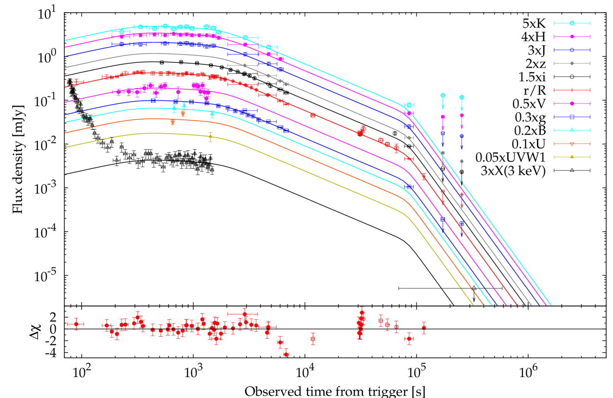
In Figure 5 we modelled the first part ( s) with a simple smoothly broken power law with a single break time, , and two power-law indices, (), taking over for at (). In order to model the later data points, we had to add a further component. A Lorentzian proved successful in this respect, so that the complete model used is given by the following equation.
| (2) |
This was used to fit the curve. The free parameters are the normalisation constant, , the break time, , two power-law indices, and , the smoothness , the Lorentzian normalisation, , the peak time, and its width, . The time-integrated flux density of the latter component is . The two terms of eq. (2) peak at and , respectively. Each of the light curves of the remaining filters were fitted with a free scaling factor with respect to the curve as modelled by eq. (2). The free parameters and the dof total 19 and 185, respectively.
The best-fit result is shown in Fig. 5, while the second line of Table 3 reports the corresponding best fit values. The fit is good: . The scaling factors for the remaining bands are the following: , , , , , , , , , , while the X-ray normalisation is still erg cm-2 s-1. The two components peak at s and ks, respectively.
We also tried to model the second component with a rising and falling smoothly broken power law instead of a Lorentzian. However, this brings in too many free parameters, such as the slope of the rise, so unless one finds reasons to fix some of them to precise values, the fit with such a component turns into highly undetermined parameters.
| /dof | |||||||||||
|---|---|---|---|---|---|---|---|---|---|---|---|
| (s) | (s) | (ks) | (ks) | (ks) | (Jy) | ||||||
| – | – | – | |||||||||
| – | – | – | – |
4.2 Spectral Energy Distribution
Figure 6 displays four SEDs we derived in as many different time intervals (see shaded bands in Fig. 3):
-
1.
SED 1 includes the last -ray pulse and the optical flash detected by RAPTOR (Wren et al. 2008), around 60 s;
-
2.
SED 2 corresponds to the final part of the optical rise, coinciding with the final part of the X-ray steep decay, spanning from to s;
-
3.
SED 3 has the broadest wavelength coverage and corresponds to the plateau phase, from to s.
-
4.
SED 4 includes NIR/visible measurements around the possible late time break in the light curve (Fig. 4), at s.
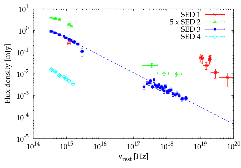
To construct SED 1 we made use of the RAPTOR measurement (Wren et al. 2008), a UVOT upper limit in the band and of the BAT spectrum of the fourth pulse. Figure 7 displays this SED: the solid line shows the best fit with a smoothed broken power law used to fit the high-energy photon spectra of the prompt emission of GRBs (Band et al. 1993).

The best-fitting parameters are the following: , and keV () consistent with the limit on derived in Sect. 3.1. The Band indices are photon indices, so the corresponding energy indices are and , respectively. While was constrained by the BAT data themselves, we solved the coupled indetermination – by initially freezing the low-energy index to the typical value of (Kaneko et al. 2006) and then leaving it to vary. The above minimum was so found. Although this does not break the degeneracy of both parameters (for every keV there is a value of for which an acceptable fit is given), here it is shown that the extrapolation of a typical Band model fitting the spectrum of the last pulse matches the optical flux observed during the flash. However, because of the lack of measurement of from -ray data, the optical flux matched by the extrapolation of the Band model may still be accidental.
The time interval of SED 2 corresponds to the first GROND frames and spans from to s (see Fig. 3). It consists of contemporaneous frames as well as X-rays.

The NIR-to-X SED 2 can be fitted with a single power-law with and negligible dust extinction. The optical data alone can be fitted with an unextinguished power law with (Table 2).
SED 3, taken during the plateau, is the richest one including all of the passbands considered in this work, but the -rays (see Fig. 3). Our NIR values are consistent with the points of Bloom & Starr (2008). Given the steadiness of the light curve and the evidence for no significant colour change along the plateau, the SED so obtained is fairly robust.

The multi-wavelength fitting of the light curves of Figs. 4 and 5 (Sect. 4.1) is dominated by the data points along the plateau phase. Thus, we built a SED using the best-fit normalisations (Sects. 4.1.1 and 4.1.2) and calculated at the time of s. We found the same results with improved uncertainties, due to the stronger constraints imposed by a multi-band fitting. The result of this SED is displayed in Figure 9. The solid line shows the best-fit model obtained adopting a rest-frame SMC-extinguished (Pei 1992), X-ray photoelectrically absorbed power law with . We note that the point corresponding to the UVW1 filter nicely agrees with the Lyman absorption at the GRB redshift. The rest-frame optical extinction was found to be negligible and a very tight limit could be derived, . Thanks to the more precise estimate obtained on , the estimate of improved correspondingly: cm-2. These results are consistent with what was obtained from the 0.3–10 keV spectrum alone and the accuracy of the estimates benefited significantly from the inclusion of NIR/visible data. Fitting the optical data alone, the result is similar: no need for a significant amount of extinction and, more importantly, the same index: (Table 2), thus ruling out the possibility of a significant reddening due to dust along the line of sight within the host galaxy.
As a consequence, two properties are inferred:
-
•
a negligible dust column density in the circumburst environment and along the line of sight to the GRB through the host galaxy;
-
•
a single power-law component accounting for the (observed) NIR to X-ray radiation, pointing to a single emission mechanism with no breaks in between. Furthermore, a single power-law spectrum implies an achromatic evolution, consistently with the observations, while the other way around is not true.
The epoch of SED 4 is ks, i.e. around the final break (aftermath of the late brightening) following the light curve description given in Sect. 4.1.1 (Sect. 4.1.2) and shown in Fig. 4 (Fig. 5). This includes optical data and is shown in Fig. 6 (diamonds). Data can be fitted either with a single unextinguished power-law with ( fixed to 0) or, alternatively, with and some extinction, . An increase of the extinction along with time seems hard to explain physically, so we are led to favour a true reddening at this time. Compared with the previous SEDs (Table 2), SED 4 is redder by (significance of ). We point out that the reddening is independent of the fit choice, as demonstrated from the comparison of the bare power-law indices with no dust correction between the earlier and later spectra (Table 2).
5 Discussion
The 15–150 keV fluence and peak flux of XRF 080330 are typical of other XRFs detected by Swift. The X-ray afterglow flux places XRF 080330 in the low end of the distribution of the GRBs observed by Swift, similarly to the majority of XRFs (Sakamoto et al. 2008). Moreover, the observed X-ray flux of XRF 080330 lies in the low end of both the XRFs sample of Swift considered by Sakamoto et al. (2008) and of the XRFs sample of BeppoSAX of D’Alessio et al. (2006). The X-ray afterglow of XRF 080330 does require a remarkable steepening after the shallow phase, with regardless of the light curve modelling (Fig. 3). This decay is typical of classical GRBs (or steeper), but is in contrast to the fairly shallow decays found by Sakamoto et al. (2008) for their sample of Swift XRFs. The optical flux of the XRF 080330 afterglow is within 1 of the distribution of the BeppoSAX XRFs sample of D’Alessio et al. (2006) at 40 ks post burst.
The coincidence of the steep decay observed in the X-ray light curve, that is a smooth continuation of the last -ray pulse, suggests that this corresponds to its high-latitude emission or the so-called “curvature effect” (Fenimore et al. 1996; Kumar & Panaitescu 2000; Dermer 2004). In the case of a thin shell emitting for a short time, the closure relation expected between temporal and spectral indices is , with the time origin reset to the ejection time of the related pulse, earlier than the onset by about 3–4 times the width of the pulse. This still holds even if the emission occurs over a finite range of radii (Genet & Granot 2008), though in that case the ratio of the ejection to pulse onset time difference and the pulse width becomes smaller ( for ).
We fitted the X-ray decay up to s with the form , where the parameters of (eq. 1) were frozen to their corresponding best-fit values obtained in Sect. 4.1.1, and the power-law parameters , and its normalisation were left free to vary. We obtained: s and s (), as shown by the solid line in Fig. 10. During the steep decay, it is (Table 2). The curvature relation is fully satisfied and we note that does correspond to the time of the last pulse. Replacing eq. (1) with eq. (2) for the underlying component, , the best-fit parameters do not change to a noticeable degree.

The optical afterglow of XRF 080330 exhibited a slow rise up to s, followed by plateau out to s, after which it decayed within a typical power-law index of about approximately out to a few s. Then, a sharp break to a decay index of occurred concurrently with an optical reddening (Sect. 4.1.1; Fig. 4). Alternatively, after the plateau a more gradual transition to a power-law decay index of set in, followed by a smooth, red bump (Sect. 4.1.2; Fig. 5). We discuss each phase separately in the following subsections.
5.1 Optical afterglow rise
In the context of the fireball model (e.g. Mészáros 2006 and references therein), the possibility that the peak of the optical afterglow emission corresponds to the passage of the peak synchrotron frequency is ruled out by the lack of spectral evolution: should evolve from negative () to positive values, while we find no evidence for changing before s.
Another possible interpretation of the optical peak is the onset of the afterglow, as for GRB 060418 and GRB 060607A (Molinari et al. 2007; Jin & Fan 2007) and, possibly, for XRF 071010A as well (Covino et al. 2008). In the case of XRF 080330, the rise during the pre-deceleration of the fireball within an ISM is much shallower than , expected at frequencies between and (Sari & Piran 1999; Granot 2005; Jin & Fan 2007). A wind environment would fit in a better way the slow rise of XRF 080330. Under these assumptions and in the thin shell case as the duration of the GRB is much shorter than the deceleration time, we can estimate the initial Lorentz factor, (approximately, twice as large as the Lorentz factor at the peak), in a wind-shaped density profile, ( is constant), with , from the peak time and the -ray radiated energy, (Chevalier & Li 2000; Molinari et al. 2007). For consistency, only the two-component model (Sect. 4.1.2; Fig. 5) must be considered. In this case, we take the peak time of the first component, s: assuming (radiative efficiency), cm-1, it turns out , and a corresponding deceleration radius smaller than cm. As in the case of XRF 071010A, the initial Lorentz factor is smaller than those found for classical GRBs. There is no evidence for the presence of a reverse shock; should the injection frequency of the reverse shock lie within the optical passbands, it would dominate the optical flux and exhibit a fast () decay (Kobayashi & Zhang 2007), not observed here. Nonetheless, this can still be the case if the injection frequency lies below the optical bands (Jin & Fan 2007; Mundell et al. 2007). A weak point of this interpretation is that the case is ruled out: (Granot 2005). Inverting this relation, a value of is required to explain the observed . This argument, together with the absence of reverse shock, whose should be much larger compared with the forward shock by a factor of (although see above), makes the interpretation of a deceleration through a wind environment somewhat contrived.
In the context of a single jet viewed off-axis (Granot et al. 2005), the rising part of the XRF 080330 curve is explained by the emission coming from the edge of the jet: as the bulk Lorentz factor decreases, the beaming cone gets progressively wider, thus resulting in a rising flux. The peak in the light curve is reached when it is , where and are the viewing and jet opening angles, respectively. According to the optical afterglow classification given by Panaitescu & Vestrand (2008), XRF 080330 belongs to the class of slow-rising and peaking after 100 s events. Those authors found a possible anti-correlation between the peak flux and the peak time for a number of fast-rising afterglows, followed also by the slow-rising class and, in this respect, XRF 080330 is no exception. The suggested interpretation of the rise is either the pre-deceleration synchrotron emission or the emergence of a highly collimated outflow seen off-axis. In the latter case, assuming a power-law angular distribution of the kinetic energy, (), high values for correspond to slower rises and dimmer peak fluxes, for a fixed off-axis viewing angle (). In the former case, the anti-correlation is ascribed to different circumburst environment densities for different events: XRF 080330, because of the negligible dust extinction, would lie in the high-peak flux region, which is not the case. This favours the interpretation of an off-axis jet whose angular distribution of energy quickly drops away from the jet axis.
An example of another XRF whose optical counterpart showed a very similar behaviour is XRR 030418. The rise of this XRR, for which only an upper limit to its redshift () was obtained (Dullighan et al. 2003), has been interpreted as due to the decreasing extinction along with time, caused by the dust column density crossed by the fireball during its expansion (Rykoff et al. 2004). Figure 11 shows the light curve compared with that of XRF 080330.
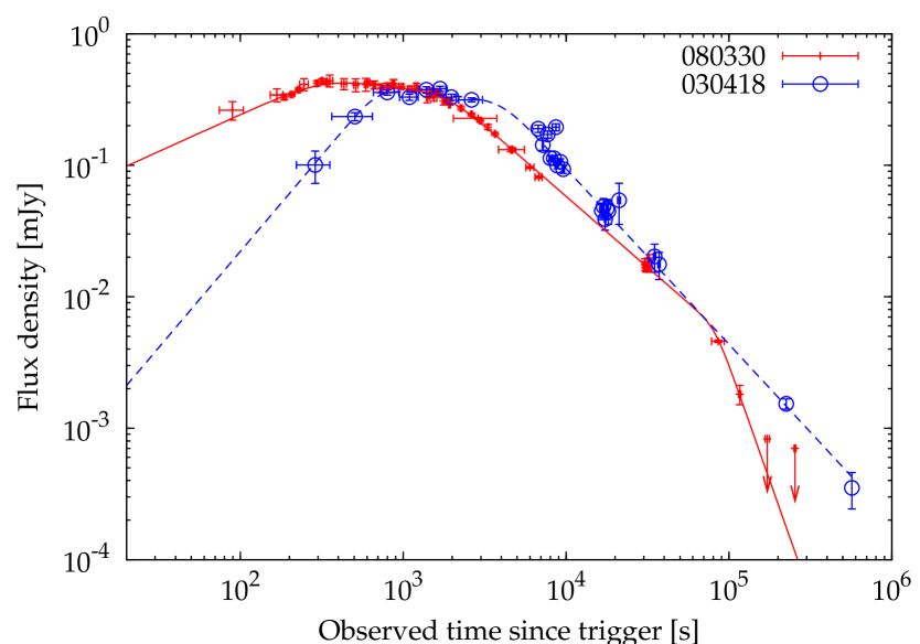
The solid line shows the best fit to the curve of XRF 080330 of Sect. 4.1.1, while the dashed line shows the same model applied to the XRR 030418 data. XRR 030418 displays a steeper rise (), which strongly depends on the zero time and could be the same as that of XRF 080330 if the time origin was moved by s forward in time (lab frame). However, there is nothing around this time in the -ray light curve of XRR 030418. Apart from the different slopes of the rise and the lack of a late-time steepening in the case of XRR 030418, the plateau and post-plateau decay look very similar. If both XRFs are caused by the same process, from the spectral (lack of) evolution XRF 080330 during the rise-plateau-initial decay phases we can rule out the decreasing dust column density hypothesis.
5.2 Plateau
From the SED extracted around the plateau no break is found between optical and X-ray frequencies, with . In the regime of slow cooling it is reasonable to assume that both optical () and X-ray () frequencies lie between the injection () and the cooling () frequencies: (Sari et al. 1998). The power-law index of the electron energy distribution, , is given by , yielding , fully within the range of values found for other bursts (e.g. Starling et al. 2008). The temporal decay index depends on the density profile: the ISM (wind) case predicts a value of (). After the plateau, depending on the light curve modelling, the measured decay index is either (Sect. 4.1.1; Fig. 4) or (Sect. 4.1.2; Fig. 5). While the multiple smoothly broken power-law description (Sect. 4.1.1) definitely rules out the wind environment, both environments are still possible in the two-component model (Sect. 4.1.2), mainly because of the poorly measured decay index, . If one interprets the flat decay as due to energy injection (Nousek et al. 2006; Zhang et al. 2006), the corresponding index would be .
In the off-axis jet interpretation, even if we consider an initially uniform sharp-edged jet, the shocked external medium at the sides of the jet has a significantly smaller Lorentz factor than near the head of the jet, and therefore its emission is not strongly beamed away from off-beam lines of sight. As a result, either an early very shallow rise or decay is expected for a realistic jet structure and dynamics (Eichler & Granot 2006). In the case of XRF 030723, Granot et al. (2005) showed that, for , an initial plateau is expected in the light curve.
Our observations of the afterglow rise of XRF 080330 rule out the interpretation proposed by Yamazaki (2009) of the plateau as due to an artifact of the choice of the reference time, as all the other rising curves do.
5.3 Jet break
According to the light curve description of Sect. 4.1.1 shown in Fig. 4, for which only an ISM environment is possible (Sect. 5.2), after the plateau phase the light curve is expected to approach the on-axis light curve with . The late-time steepening observed around s, estimated to be , cannot be produced by the passage of the cooling frequency through the optical, as that is expected to be as small as (ISM/wind).
In the off-axis jet interpretation, assuming a value for of a few degrees, another advantage of this interpretation is the steep late time decay (at 1 day) as a consequence of joining the post jet break on-axis light curve. According to the light curve modelling given in Sect. 4.1.2 shown in Fig. 5, the gradual steepening following the plateau corresponds to the post-jet break emission: the observed power-law decay index, is consistent with the expected . We note that the relatively sharp jet break favours the ISM environment. Overall, in the context of an off-axis viewing angle interpretation, the light curve suggests that as well as an early jet break (at day), which in turn implies a narrow jet with a half-opening angle of the order of a few degrees, . As a simple feasibility check, we note that for the ratio of the on-axis to off-axis is equal to (assuming that the observed energy range includes where most of the energy is radiated), where is the ratio of their corresponding Doppler factors and therefore of their (Eichler & Levinson 2004). In our case, for an observed off-axis keV, an on-axis value of MeV would require and , which for and gives . Here is the initial Lorentz factor at the edge of the jet. More realistically, the jet would not be perfectly uniform with extremely sharp edges, and instead is expected to be lower at the outer edge of the jet and larger near its center (where it could easily reach several hundreds in our illustrative example here). In this case so that the observed in the keV range, which is erg, would imply an on-axis value for of erg, which for a narrow jet with would correspond to a true energy of the order of erg. This demonstrates that this scenario can work for reasonable values of the physical parameters. We point out that the estimate of the on-axis of erg is for a wide energy range containing , since in our illustrative example most of the energy is released within the observed range. A more accurate estimate of the break time and of the corresponding opening angle is difficult, due to the degeneracy involved in the light curve modelling (Figs. 4 and 5). Table 4 summarises the main properties of XRF 080330.
| Name | Value |
|---|---|
| erg cm-2 | |
| ph cm-2 s-1 | |
| keV | |
| keV | |
| (– keV, obs frame) | ergs |
| (– keV, GRB frame) | ergs |
| (obs frame) | day |
| (jet opening angle)(a) | few degrees |
| (viewing angle)(a) |
5.4 Late time red bump
Overall, the two-component description of the light curves of Sect. 4.1.2 shown in Fig. 5 appears to be slightly favoured over the multiple smoothly broken power-law of Fig. 4. So, irrespective of the nature of the rise and plateau, we speculate on the possible nature of the second component, modelled in Fig. 5 as a late time bump. Clearly, a SN bump, such as that possibly observed in the light curve of XRF 030723 (Fynbo et al. 2004), is ruled out mainly because that is expected to peak days later, which is incompatible with one single day after XRF 080330; not to mention the too high redshift of XRF 080330 for a 1998bw-like SN to be detected.
Alternatively, a density bump seems a viable solution, given that (e.g. Lazzati et al. 2002; Guidorzi et al. 2005), although the explanation of the observed contemporaneous reddening requires ad hoc assumptions, such as the case of GRB 050721, which showed similar properties to XRF 080330 (same with no breaks between optical and X-ray, late time redder optical bump). In that case, the observed reddening was explained as due to the presence of very dense clumps surviving the GRB radiation and with a small covering factor (Antonelli et al. 2006).
If the late reddening is due to the passage of through the optical bands, in addition to what argued in Sect. 5.3, another weak point of the multiple smoothly broken power-law description of Fig. 4 (Sect. 4.1.1) is the chromatic change of we observe in the optical bands around s. The passage of the cooling frequency does not explain it: the observed reddening would be 0.5, i.e. twice as much. This could still be the case, if our measurement might have taken place in the course of the spectral change, as the broken power-law spectrum is a simple approximation. However, since it is during the plateau because of the unbroken power-law spectrum between optical and X-ray, would have decreased very rapidly, thus making this option not reasonable: if at s it is Hz, at s it should be Hz , because (ISM case), thus this possibility is to be ruled out. Likewise, in the wind case it is . The times and , at which would cross the most redward and blueward filters, and , would differ by a factor of , which looks incompatible with the light curves. Furthermore, the observed reddening rules out the wind case, as should decrease from to .
Although an energy injection to the blast wave (forward shock) can explain the bump feature in the light curve, it is difficult to explain the reddening if we consider only the forward shock emission, as we have discussed. A possible explanation for the reddening is that the rebrightening is due to the short-lived () reverse shock of a slow shell which caught up with the shock front and increased its energy through a refreshed shock (e.g. Kumar & Piran 2000; Granot et al. 2003; Jóhannesson et al. 2006): since that shock is going into a shell of ejecta, rather than the external medium, it can have a much larger (magnetised fireball: Zhang et al. 2003; Kumar & Panaitescu 2003; Gomboc et al. 2008b) and, therefore, a lower , quite naturally; for an ISM where decreases with time, then of the reverse shock could be around the optical for reasonable model parameter values. The need for a separate component to explain a chromatic break in the light curve was also suggested in the case of GRB 061126 (Gomboc et al. 2008b). Notably, the final steepening after s, which in the modelling of Sect. 4.1.1 (Fig. 4) is described with , is compatible with the high-latitude emission of the reverse shock: . The jet break might happen slightly earlier than the break time in the optical light curve.
A somewhat more contrived way to explain the bump is the appearance of a second narrower jet in the two-component jet model, as proposed for XRF 030723 (Huang et al. 2004). In this model, the viewing angle, is within or slightly off the cone of the wide jet and outside the narrow jet. The plateau phase would reflect the deceleration of the wide jet (Granot et al. 2006). Depending on the isotropic-equivalent kinetic energy of the wide and narrow jet, and , on the jet opening angles, and , on the initial bulk Lorentz factors, and , respectively, as well as on the viewing angle, the afterglow emission of either component is dominant at different times. According to the results of Huang et al. (2004), the light curve of XRF 080330 could be qualitatively explained as follows: the first component obtained in Sect. 4.1.2 (Fig. 5) represents the contribution of the wide jet dominating at early times: the rise could be due either to the afterglow onset (in a wind environment) or to a viewing angle slightly beyond the wide jet opening angle: . The appearance of the second component would mark the deceleration and lateral expansion of the narrow jet, the peak time corresponding to the case . Unlike XRF 030723, which showed a relatively sharp late-time peak, the bump exhibited by XRF 080330 looks less sharp and pronounced. Although this might suggest a relatively lower energy of the narrow jet compared to XRF 030723, yet we cannot exclude the case . The ratio of the observed energies of XRF 080330, of about according to the modelling of Sect. 4.1.2, corresponds to the ratio between the early and the late time emissions of the wide and narrow jets, respectively. Depending on the values of , , , a comparable ratio of observed energies, such as that observed for XRF 080330, can still be obtained in the case of a much more energetic narrow jet, .
Such a model turned out to be successful in accounting for the naked-eye GRB 080319B (Racusin et al. 2008): in that case, the two collimation-corrected energies were comparable, while the isotropic-equivalent energy of the narrow jet () was about 400 times larger than that of the wide jet ().
However, in the context of the two-component model the explanation of the late time reddening simultaneously with the appearance of the narrow component emission requires two different values of for the two jets, which does not look reasonable on a physical ground. Another option is that the cooling frequency of the second jet might be around the optical at the time of the bump: however, if the shock micro-physics parameters (, , ), are the same for the two shocks, as expected on physical grounds, and obviously the external medium is the same, then the only thing that is different as far as is concerned, is . Since the presence of the bump requires , then this would not work for the wind case, where . Even in the ISM case, where , the fact that at s, and therefore Hz at s for the wide jet, requires (which is very extreme) in order for to be around Hz (required by the observed reddening). Therefore, while this could work in principle, in practise it requires extreme parameters. In particular, the amplitude of the bump suggests that , and therefore from the required it would follow , which seems pushed to the extreme.
Overall, these considerations make the single off-axis jet interpretation much more compelling.
6 Conclusions
XRF 080330 is representative of the XRR and XRF classes of soft GRBs. Its - and X-ray properties of both prompt and high-energy afterglow emission place it in the low-flux end of the distribution. The multi-band (NIR through UV) optical curve showed an initial rise up to 300 s, followed by a 2-ks long plateau, temporally coinciding with the canonical flat decay of X-ray afterglows of all kinds of GRBs, followed by a gradual steepening and a possible jet break. We provided two alternative descriptions of the light curve: a piecewise power-law with three break times, the last of which occurring around s and followed by a sharp steepening, with the power-law decay index changing from to . The SED from NIR to X-ray wavelength is fitted with a simple power-law with and negligible GRB-frame extinction, adopting a SMC-like profile, with no evidence for chromatic evolution during the rise, plateau and early ( s) decay phases. However, after the possible late time break we observe a reddening in the optical bands of , which cannot be accounted for in terms of the synchrotron spectrum evolution of a standard afterglow model, unless a different description of the light curve is considered. In the alternative model of the light curves, we identified two distinct components: the first is modelled with a smoothly broken power law and fits the rise plateau and early decay of the afterglow, while the second, taking over around s, is modelled with an energy injection episode peaking at ks and with a time-integrated energy of 60% that of the first component.
The X-ray light curve consists of the initial steep decay, which is likely the high-latitude emission of the last -ray pulse. At the same time, the optical afterglow rises up to a plateau, temporally coincident with the X-ray flat decay. In this case, we collected strong evidence that the emission mechanism during this phase is the same from optical to X-rays and is consistent with synchrotron emission of a decelerating fireball with an electron energy distribution power-law index of .
The lack of spectral evolution throughout the rise, plateau and early decay argue against a temporally decreasing dust column density claimed to explain similar optical light curves of past soft bursts.
The optical rise () is too slow for the afterglow onset within a uniform circumburst medium, but could still be the case if a wind environment is considered. In this case, under standard assumptions we constrained the Lorentz factor of the fireball to be smaller than 80, thus confirming the scenario of XRFs as less relativistic GRBs. However, we found that the interpretation of a single-component off-axis jet with an opening angle of a few degrees and a viewing angle about twice as large, can explain the observations: this not only accounts for the light curve morphology, but also explains the soft nature of XRF of the -ray prompt event. The reddening observed at s can be interpreted as the short-lived reverse shock of an energy injection caused by a slow shell which caught up with the fireball shock front, also responsible for the contemporaneous bump in the light curve. A two-component jet could also work, but would introduce more free parameters and would require extreme conditions.
The interpretation of the late bump as produced by a density enhancement in the medium swept up by the fireball cannot be ruled out, although the reddening seems to require ad hoc explanations. In this case, as shown by Nakar & Granot (2007), it is hard to produce a flux enhancement with density inhomogeneities, although it is not excluded given the lack of a sharp rise in this bump.
Overall, the XRF 080330 optical and X-ray afterglows properties have also been observed in many other GRBs (Panaitescu & Vestrand 2008). This both supports the view of a common origin of XRFs and classical GRBs, which form a continuum and do not call for distinct mechanisms. The importance of a prompt multi-wavelength coverage of the early phases of a GRB is clearly demonstrated in the case of XRF 080330.
Acknowledgements.
This work is supported by ASI grant I/R/039/04 and by the Ministry of University and Research of Italy (PRIN 2005025417). JG gratefully acknowledges a Royal Society Wolfson Research Merit Award. DARK is funded by the DNRF. PJ acknowledges support by a Marie Curie European Re-integration Grant within the 7th European Community Framework Program under contract number PERG03-GA-2008-226653, and a Grant of Excellence from the Icelandic Research Fund. We gratefully acknowledge the contribution of the Swift team members at OAB, PSU, UL, GSFC, ASDC, MSSL and our sub-contractors, who helped make this mission possible. We acknowledge Sami-Matias Niemi for executing the NOT observations. CG is grateful to A. Kann for his reading and comments.References
- Amati et al. (2002) Amati, L., Frontera, F., Tavani, M., et al. 2002, A&A, 390, 81
- Amati et al. (2004) Amati, L., Frontera, F., in ’t Zand, J. J. M., et al. 2004, A&A, 426, 415
- Amati (2006) Amati, L. 2006, MNRAS, 372, 233
- Amati et al. (2007) Amati, L., Della Valle, M., Frontera, F., et al. 2007, A&A, 463, 913
- Antonelli et al. (2006) Antonelli, L. A., Testa, V., Romano, P., et al. 2006, A&A, 456, 509
- Band et al. (1993) Band, D., Matteson, J., Ford, L., et al. 1993, ApJ, 413, 281
- Barraud et al. (2003) Barraud, C., Olive J.-F., Lestrade, J. P., et al. 2003, A&A, 400, 1021
- Barthelmy et al. (2005) Barthelmy, S. D., Barbier, L. M., Cummings, J. R., et al. 2005, Space Sci. Rev., 120, 143
- Berger et al. (2003) Berger, E., Kulkarni, S. R., Pooley, G., et al. 2003, Nature, 426, 154
- Bertin & Arnouts (1996) Bertin, E., & Arnouts, S. 1996, A&AS, 117, 393
- Beuermann et al. (1999) Beuermann, K., Hessman, F.V., Reinsch, K., et al. 1999, A&A, 352, L26
- Bloom & Starr (2008) Bloom, J. S., & Starr, D. L. 2008, GCN Circ., 7542
- Burrows et al. (2005) Burrows, D. N., Hill, J. E., Nousek, J. A., et al. 2005, Space Sci. Rev., 120, 165
- Butler et al. (2005) Butler, N.R., Sakamoto, T., Suzuki, M., et al. 2005, ApJ, 621, 884
- Campana et al. (2006) Campana, S., Mangano, V., Blustin, A. J., et al. 2006, Nature, 442, 1008
- Cardelli et al. (1989) Cardelli, J. A., Clayton, G. C., & Mathis, J. S. 1989, ApJ, 345, 245
- Chevalier & Li (2000) Chevalier, R. A., & Li, Z.-Y. 2000, ApJ, 536, 195
- Clemens et al. (2008) Clemens, C., Küpcü Yoldaş, A., Greiner, J., Yoldaş, A., Krühler, T., Szokoly, G., 2008, GCN Circ., 7545
- Cool et al. (2008) Cool, R. J., Eisenstein, D. J., Hogg, D. W., et al. 2008, GCN Circ., 7540
- Covino et al. (2008) Covino, S., D’Avanzo, P., Klotz, A., et al. 2008, MNRAS, 388, 347
- Cucchiara & Fox (2008) Cucchiara, A. & Fox, D. B. 2008, GCN Circ., 7547
- D’Alessio et al. (2006) D’Alessio, V., Piro, L., & Rossi, E. M. 2006, A&A, 460, 653
- D’Avanzo et al. (2008) D’Avanzo, P., Covino, S., Fugazza, D., et al. 2008, GCN Circ., 7554
- Della Valle et al. (2006) Della Valle, M., Chincarini, G., Panagia, N., et al. 2006, Nature, 444, 1050
- De Pasquale et al. (2007) De Pasquale, M., Oates, S.R., Page, M.J., et al. 2007, MNRAS, 377, 1638
- Dermer (2004) Dermer, C.D. 2004, ApJ, 614, 284
- Dermer et al. (2000) Dermer, C. D., Chiang, J., & Mitman, K. E. 2000, ApJ, 537, 785
- Devillard (2001) Devillard, N. 2001, ASP Conf. Ser., 238, 525
- Donaghy (2006) Donaghy, T. Q. 2006, ApJ, 645, 436
- Dullighan et al. (2003) Dullighan, A., Butler, N. R., Ricker, G. R., et al. 2003, GCN Circ., 2236
- Eichler & Levinson (2004) Eichler, D., & Levinson, A. 2004, ApJ, 614, L13
- Eichler & Granot (2006) Eichler, D., & Granot, J. 2006, ApJ, 641, L5
- Fenimore et al. (1996) Fenimore, E.E., Madras, C.D., & Nayakshin, S. 1996, ApJ, 473, 998
- Ferrero et al. (2003) Ferrero, P., Pizzichini, G., Bartolini, C., et al. 2003, GCN Circ., 2284
- Fox et al. (2003) Fox, D.W., Yost, S.A., Kulkarni, S.R., et al. 2003, Nature, 422, 284
- Frontera et al. (2000) Frontera, F., Antonelli, L. A., Amati, L., et al. 2000, ApJ, 540, 697
- Fukugita et al. (1996) Fukugita, M., Ichikawa, T., Gunn, J.E., et al. 1996, AJ, 111, 1748
- Fynbo et al. (2004) Fynbo, J. P. U., Sollerman, J., Hjorth, J., et al. 2004, ApJ, 609, 962
- Fynbo et al. (2006) Fynbo, J. P. U., Watson, D., Thöne, C., et al. 2006, Nature, 444, 1047
- Gal-Yam et al. (2006) Gal-Yam, A., Fox, D. B., Price, P. A., et al. 2006, Nature, 444, 1053
- Gehrels et al. (2004) Gehrels, N., Chincarini, G., Giommi, P. et al. 2004, ApJ, 611, 1005
- Genet et al. (2007) Genet, F., Daigne, F., & Mochkovitch, R. 2007, MNRAS, 381, 732
- Genet & Granot (2008) Genet, F., & Granot, J. 2008, submitted (arXiv:0812.4677)
- Ghirlanda et al. (2004) Ghirlanda, G., Ghisellini, G., & Lazzati, D. 2004, ApJ, 616, 331
- Ghisellini et al. (2007) Ghisellini, G., Ghirlanda, G., Nava, L., & Firmani, C. 2007, ApJ, 658, L75
- Ghisellini et al. (2009) Ghisellini, G., Nardini, M., Ghirlanda, G., & Celotti, A. 2009, MNRAS, 393, 253
- Gomboc et al. (2006) Gomboc, A., Guidorzi, C., Mundell, C.G., et al. 2006, Il Nuovo Cimento C, 121B, 1303
- Gomboc et al. (2008a) Gomboc, A., Guidorzi, C., Melandri, A., et al. 2008a, GCN Circ., 7539
- Gomboc et al. (2008b) Gomboc, A., Kobayashi, S., Guidorzi, C., et al. 2008b, ApJ, 687, 443
- Granot et al. (2002) Granot, J., Panaitescu, A., Kumar, P., & Woosley, S. 2002, ApJ, 570, L61
- Granot et al. (2003) Granot, Y., Nakar, E., & Piran, T. 2003, Nature, 426, 138
- Granot (2005) Granot, J. 2005, ApJ, 631, 1022
- Granot et al. (2005) Granot, J., Ramirez-Ruiz, E., & Perna, R. 2005, ApJ, 630, 1003
- Granot & Kumar (2006) Granot, J., & Kumar, P. 2006, MNRAS, 366, L13
- Granot et al. (2006) Granot, J., Königl, A., & Piran, T. 2006, MNRAS, 370, 1946
- Greiner et al. (2008) Greiner, J., Bornemann, W., Clemens, C., et al. 2008, PASP, 120, 405
- Guidorzi et al. (2005) Guidorzi, C., Monfardini, A., Gomboc, A., et al. 2005, ApJ, 630, L121
- Guidorzi et al. (2006) Guidorzi, C., Monfardini, A., Gomboc, A., et al. 2006, PASP, 118, 288
- Heise et al. (2001) Heise, J., in’ t Zand, J., Kippen, R.M., & Woods, P.M. 2001, in Gamma-Ray Bursts in the Afterglow Era, ed. E. Costa, F. Frontera, & J. Hjorth (Berlin: Springer), 16
- Huang et al. (2004) Huang, Y.F., Wu, X.F., Dai, Z.G., Ma, H.T., & Lu, T. 2004, ApJ, 605, 300
- Im et al. (2008) Im, M., Lee, I., Urata, Y., et al. 2008, GCN Circ., 7546
- Ioka et al. (2006) Ioka, K., Toma, K., Yamazaki, R., & Nakamura, T. 2006, A&A, 458, 7
- Jóhannesson et al. (2006) Jóhannesson, G., Björnsson, G., & Gudmundsson, E.H. 2006, ApJ, 647, 1238
- Jin & Fan (2007) Jin, Z. P., & Fan, Y. Z. 2007, MNRAS, 378, 1043
- Kalberla et al. (2005) Kalberla, P.M.W., Burton, W.B., Hartmann, D., et al. 2005, A&A, 440, 775
- Kaneko et al. (2006) Kaneko, Y., Preece, R.D., Briggs, M.S., et al. 2006, ApJS, 166, 298
- Klotz et al. (2008a) Klotz, A., Boër, M., Atteia, J.L. 2008a, GCN Circ., 7536
- Klotz et al. (2008b) Klotz, A., Boër, M., Atteia, J.L. 2008b, GCN Circ., 7543
- Klotz et al. (2008c) Klotz, A., Boër, M., Eysseric, J., et al., 2008, PASP, 120, 1298
- Kobayashi & Zhang (2007) Kobayashi, S., & Zhang, B., 2007, ApJ, 655, 973
- Krisciunas et al. (1998) Krisciunas, K., Margon, B., & Szkody, P. 1998, PASP, 110, 1342
- Kumar & Panaitescu (2000) Kumar, P., & Panaitescu, A. 2000, ApJ, 541, L51
- Kumar & Panaitescu (2003) Kumar, P., & Panaitescu, A. 2003, MNRAS, 346, 905
- Kumar & Piran (2000) Kumar, P., & Piran, T. 2000, ApJ, 532, 286
- Landolt (1992) Landolt, A.U., 1992, AJ, 104, 340
- Lazzati et al. (2002) Lazzati, D., Rossi, E., Covino, S., Ghisellini, G., & Malesani, D. 2002, A&A, 396, L5
- Levan et al. (2005) Levan, A., Patel, S., Kouveliotou, C., et al. 2005, ApJ, 622, 977
- Malesani et al. (2008) Malesani, D., Fynbo, J. P. U., Jakobsson, P., Vreeswijk, P. M. 2008, GCN Circ., 7544
- Mangano et al. (2007) Mangano, V., La Parola, V., Cusumano, G., et al. 2007, ApJ, 654, 403
- Mao & Guidorzi (2008) Mao, J., & Guidorzi, C. 2008, GCN Circ., 7583
- Mao et al. (2008a) Mao, J., Baumgartner, W. H., Burrows, D. N., et al. 2008a, GCN Circ. 7537
- Mao et al. (2008b) Mao, J., Guidorzi, C., Markwardt, C., Kuin, N. P. M., Barthelmy, S. D., Burrows, D. N., Roming, P., Gehrels, N. 2008b, GCN Report, 132.1
- Markwardt et al. (2008) Markwardt, C., Barthelmy, S.D., Cummings, J., et al. 2008, GCN Circ., 7549
- Mészáros (2006) Mészáros, P. 2006, Rep. Prog. Phys. 2006, 69, 2259
- Mochkovitch et al. (2004) Mochkovitch, R., Daigne, F., Barraud, C., & Atteia, J.-L. 2004, ASP Conf. Ser., 312, 381
- Molinari et al. (2007) Molinari, E., Vergani, S.D., Malesani, D. et al. 2007, A&A, 469, L13
- Morrison & McCammon (1983) Morrison, R., & McCammon, D. 1983, ApJ, 270, 119
- Moskvitin et al. (2008) Moskvitin, A.S., Fatkhullin, T.A., Komarova, V.N., & Burenkov, A.N. 2008, GCN Circ., 7559
- Mundell et al. (2007) Mundell, C. G., Steele, I. A., Smith, R. J., et al. 2007, Science, 315, 1822
- Nakar & Granot (2007) Nakar, E., & Granot, J. 2007, MNRAS, 380, 1744
- Norris et al. (2005) Norris, J.P., Bonnell, J.T., Kazanas, D., Scargle, J. D., Hakkila, J., & Giblin, T. W. 2005, ApJ, 627, 324
- Nousek et al. (2006) Nousek, J.A., Koveliotou, C., Grupe, D., et al. 2006, ApJ, 642, 389
- Panaitescu & Vestrand (2008) Panaitescu, A., & Vestrand, W.T. 2008, MNRAS, 387, 497
- Pei (1992) Pei, Y.C. 1992, ApJ, 395, 130
- Peng et al. (2005) Peng, F., Königl, A., & Granot, J. 2005, ApJ, 626, 966
- Pian et al. (2006) Pian, E., Mazzali, P., Masetti, N. et al. 442, Nature, 1011
- Poole et al. (2008) Poole, T.S., Breeveld, A.A., Page, M.J., et al. 2008, MNRAS, 383, 627
- Preece et al. (2000) Preece, R. D., Briggs, M. S., Pendleton, G. N., Paciesas, W. S. 2000, ApJS, 126, 19
- Racusin et al. (2008) Racusin, J. L., Karpov, S. V., Sokolowski, M., et al. 2008, Nature, 455, 183
- Roming et al. (2005) Roming, P. W. A., Kennedy, T. E., Mason, K. O., et al. 2005, Space Sci. Rev., 120, 95
- Rykoff et al. (2004) Rykoff, E.S., Smith, D.A., Price, P.A., et al. 2004, ApJ, 601, 1013
- Romano et al. (2006) Romano, P., Moretti, A., Banat, P.L. et al. 2006, A&A, 450, 59
- Rossi et al. (2008) Rossi, F., Guidorzi, C., Amati, L., et al. 2008, MNRAS, 388, 1284
- Sakamoto et al. (2005) Sakamoto, T., Lamb, D. Q., Kawai, N., et al. 2005, ApJ, 629, 311
- Sakamoto et al. (2008) Sakamoto, T., Hullinger, D., Sato, G., et al. 2008, ApJ, 679, 570
- Sakamoto et al. (2009) Sakamoto, T., Sato, G., Barbier, L., et al. 2009, ApJ, 693, 922
- Salmonson (2003) Salmonson, J. D. 2003, ApJ, 592, 1002
- Sari et al. (1998) Sari, R., Piran, T., & Narayan, R. 1998, ApJ, 497, L17
- Sari & Piran (1999) Sari, R., & Piran, T. 1999, ApJ, 520, 641
- Schaefer et al. (2008) Schaefer, B. E., & Guver, T. 2008, GCN Circ., 7538
- Schlegel et al. (1998) Schlegel, D. J., Finkbeiner, D. P., & Davis, M. 1998, ApJ, 500, 525
- Schubel et al. (2008) Schubel, M., Reichart, D., Nysewander, M., et al. 2008, GCN Circ., 7560
- Sergeev et al. (2008) Sergeev, A., Andreev, M., Petkov, V., Kurenya, A., & Pozanenko, A. 2008, GCN Circ., 7556
- Shao & Dai (2007) Shao, L., & Dai, Z. G. 2007, ApJ, 660, 1319
- Starling et al. (2008) Starling, R. L. C., van der Horst, A. J., Rol, E., et al. 2008, ApJ, 672, 433
- Tagliaferri et al. (2005) Tagliaferri, G., Goad, M., Chincarini, G. et al. 2005, Nature, 436, 985
- Tominaga et al. (2004) Tominaga, N., Deng, J., Mazzali, P.A., et al. 2004, ApJ, 612, L105
- Troja et al. (2007) Troja, E., Cusumano, G., O’Brien, P. T., et al. 2007, ApJ, 665, 599
- Uhm & Beloborodov (2007) Uhm, L. Z., & Beloborodov, A. M. 2007, ApJ, 665, L93
- Wang et al. (2008) Wang, X.F., Li, J.Z., Feng, Q.C., et al. 2008, GCN Circ., 7550
- Wren et al. (2008) Wren, J., Vestrand, W. T., Wozniak, P. R., & Davis, H. 2008, GCN Circ., 7568
- Yamazaki (2009) Yamazaki, R. 2009, ApJ, 690, L118
- Yamazaki et al. (2002) Yamazaki, R., Ioka, K., & Nakamura, T. 2002, ApJ, 571, L31
- Yuan et al. (2008) Yuan, F., Rykoff, E. S., Schaefer, B. E., et al. 2008, in AIP Conf. Proc., 1065, 2008 Nanjing Gamma-Ray Burst Conference, eds. Y.-F. Huang, Z.-G. Dai, & B. Zhang, 103
- Zhang (2007) Zhang, B. 2007, Chinese J. Astron. Astrophys., 7, 1
- Zhang et al. (2003) Zhang, B., Kobayashi, S., & Mészáros, P. 2003, ApJ, 595, 950
- Zhang et al. (2006) Zhang, B., Fan, Y.Z., Dyks, J., et al. 2006, ApJ, 642, 354
- Zerbi et al. (2001) Zerbi, F.M., Chincarini, G., Ghisellini, G., et al. 2001, Astron. Nach., 322, 275
| Mid time | Exposure | Magnitudea,b | Filter | Telescope |
|---|---|---|---|---|
| (s) | (s) | |||
| SDSS- | LT | |||
| SDSS- | LT | |||
| SDSS- | LT | |||
| SDSS- | LT | |||
| SDSS- | LT | |||
| SDSS- | LT | |||
| SDSS- | LT | |||
| SDSS- | LT | |||
| SDSS- | LT | |||
| SDSS- | LT | |||
| SDSS- | LT | |||
| SDSS- | LT | |||
| SDSS- | LT | |||
| SDSS- | LT | |||
| SDSS- | LT | |||
| SDSS- | LT | |||
| SDSS- | LT | |||
| SDSS- | LT | |||
| SDSS- | LT | |||
| SDSS- | LT | |||
| SDSS- | LT | |||
| SDSS- | LT | |||
| SDSS- | LT | |||
| SDSS- | LT | |||
| SDSS- | LT | |||
| SDSS- | LT | |||
| SDSS- | LT | |||
| SDSS- | LT | |||
| SDSS- | LT | |||
| SDSS- | FTN | |||
| SDSS- | FTN | |||
| SDSS- | FTN | |||
| SDSS- | FTN | |||
| SDSS- | FTN | |||
| SDSS- | FTN | |||
| SDSS- | FTN | |||
| SDSS- | FTN | |||
| SDSS- | FTN | |||
| SDSS- | FTN | |||
| SDSS- | FTN | |||
| SDSS- | LT | |||
| SDSS- | LT | |||
| SDSS- | LT | |||
| SDSS- | LT | |||
| SDSS- | LT | |||
| SDSS- | LT | |||
| SDSS- | LT | |||
| SDSS- | LT | |||
| SDSS- | LT | |||
| SDSS- | LT | |||
| SDSS- | LT | |||
| SDSS- | LT | |||
| SDSS- | FTN | |||
| SDSS- | GROND | |||
| SDSS- | GROND | |||
| SDSS- | GROND | |||
| SDSS- | GROND | |||
| SDSS- | GROND | |||
| SDSS- | GROND | |||
| SDSS- | GROND | |||
| SDSS- | GROND | |||
| SDSS- | GROND | |||
| SDSS- | GROND | |||
| SDSS- | GROND | |||
| SDSS- | GROND | |||
| SDSS- | GROND | |||
| SDSS- | GROND | |||
| SDSS- | GROND | |||
| SDSS- | GROND | |||
| SDSS- | GROND | |||
| SDSS- | GROND | |||
| SDSS- | GROND | |||
| SDSS- | GROND | |||
| SDSS- | GROND | |||
| SDSS- | GROND | |||
| SDSS- | GROND | |||
| SDSS- | GROND | |||
| SDSS- | GROND | |||
| SDSS- | GROND | |||
| SDSS- | GROND | |||
| SDSS- | GROND | |||
| GROND | ||||
| GROND | ||||
| GROND | ||||
| GROND | ||||
| GROND | ||||
| GROND | ||||
| GROND | ||||
| GROND | ||||
| GROND | ||||
| GROND | ||||
| GROND | ||||
| GROND | ||||
| GROND | ||||
| GROND | ||||
| GROND | ||||
| GROND | ||||
| GROND | ||||
| GROND | ||||
| GROND | ||||
| GROND | ||||
| GROND | ||||
| GROND | ||||
| GROND | ||||
| GROND | ||||
| GROND | ||||
| GROND | ||||
| GROND | ||||
| GROND | ||||
| GROND | ||||
| GROND | ||||
| GROND | ||||
| GROND | ||||
| GROND | ||||
| GROND | ||||
| GROND | ||||
| GROND | ||||
| GROND | ||||
| GROND | ||||
| GROND | ||||
| GROND | ||||
| GROND | ||||
| GROND | ||||
| GROND | ||||
| GROND | ||||
| GROND | ||||
| GROND | ||||
| GROND | ||||
| GROND | ||||
| GROND | ||||
| NOT | ||||
| NOT | ||||
| NOT | ||||
| SDSS- equivalent | REM | |||
| SDSS- equivalent | REM | |||
| SDSS- equivalent | REM | |||
| SDSS- equivalent | REM | |||
| SDSS- equivalent | REM | |||
| SDSS- equivalent | REM | |||
| SDSS- equivalent | REM | |||
| SDSS- equivalent | REM | |||
| SDSS- equivalent | REM | |||
| SDSS- equivalent | REM | |||
| SDSS- equivalent | REM | |||
| SDSS- equivalent | REM | |||
| SDSS- equivalent | REM | |||
| SDSS- equivalent | REM | |||
| SDSS- equivalent | REM | |||
| SDSS- equivalent | REM | |||
| SDSS- equivalent | REM | |||
| SDSS- equivalent | REM | |||
| clear | TAROT | |||
| clear | TAROT | |||
| clear | TAROT | |||
| clear | TAROT | |||
| clear | TAROT | |||
| clear | TAROT | |||
| TAROT | ||||
| clear | TAROT | |||
| clear | TAROT | |||
| clear | TAROT | |||
| clear | TAROT | |||
| TAROT | ||||
| clear | TAROT | |||
| clear | TAROT | |||
| TAROT | ||||
| UVOT | ||||
| white | UVOT | |||
| white | UVOT | |||
| white | UVOT | |||
| white | UVOT | |||
| white | UVOT | |||
| white | UVOT | |||
| white | UVOT | |||
| UVOT | ||||
| UVOT | ||||
| UVOT | ||||
| UVOT | ||||
| UVOT | ||||
| UVOT | ||||
| UVOT | ||||
| UVOT | ||||
| UVW1 | UVOT | |||
| UVOT | ||||
| UVOT | ||||
| white | UVOT | |||
| UVOT | ||||
| UVW1 | UVOT | |||
| UVW2 | UVOT | |||
| UVOT | ||||
| UVOT | ||||
| white | UVOT | |||
| white | UVOT | |||
| UVM2 | UVOT | |||
| UVOT | ||||
| UVOT | ||||
| UVOT | ||||
| UVOT | ||||
| UVOT | ||||
| UVOT | ||||
| UVOT | ||||
| UVOT | ||||
| UVW1 | UVOT | |||
| UVOT | ||||
| UVOT | ||||
| UVOT | ||||
| UVOT | ||||
| UVOT | ||||
| UVW1 | UVOT | |||
| white | UVOT |
-
a
Values are not corrected for Galactic extinction.
-
b
Errors at the 68% confidence level and upper limits (3 ) are given.
-
c
AB magnitudes.
| [Å] | [Å] | Feature | EW [Å] | |
|---|---|---|---|---|
| 3889.4 | 1548.2/1550.8 | 1.5101 | C iv | 4.30.7 |
| 4028.8 | 1608.5 | 1.5047 | FeII | 2.00.7 |
| 4198.2 | 1670.8 | 1.5127 | AlII | 2.00.7 |
| 5093.5 | 2026.1 | 1.5139 | Zn ii | 4.30.4 |
| 5190.3 | 2062.2 | 1.5166 | CrII | 0.60.3 |
| 5190.3 | 2062.7 | 1.5166 | ZnII | |
| 5883.4 | 2344.2 | 1.5100 | FeII | 1.40.5 |
| 5983.0 | 2382.8 | 1.5109 | FeII | 2.20.5 |
| 6497.5 | 2586.7 | 1.51 | FeII | 112 |
| 6527.0 | 2600.2 | 1.51 | FeII | |
| 7031.1 | 2796.3/2803.5 | 1.5112 | MgII | 5.20.3 |