Risk-Averse Decision Making Under Uncertainty
Abstract
A large class of decision making under uncertainty problems can be described via Markov decision processes (MDPs) or partially observable MDPs (POMDPs), with application to artificial intelligence and operations research, among others. Traditionally, policy synthesis techniques are proposed such that a total expected cost/reward is minimized/maximized. However, optimality in the total expected cost sense is only reasonable if system’s behavior in the large number of runs is of interest, which has limited the use of such policies in practical mission-critical scenarios, wherein large deviations from the expected behavior may lead to mission failure. In this paper, we consider the problem of designing policies for MDPs and POMDPs with objectives and constraints in terms of dynamic coherent risk measures, which we refer to as the constrained risk-averse problem. Our contributions are fourfold:
-
(i)
For MDPs, we reformulate the problem into a inf-sup problem via the Lagrangian framework. Under the assumption that the risk objectives and constraints can be represented by a Markov risk transition mapping, we propose an optimization-based method to synthesize Markovian policies;
-
(ii)
For MDPs, we demonstrate that the formulated optimization problems are in the form of difference convex programs (DCPs) and can be solved by the disciplined convex-concave programming (DCCP) framework. We show that these results generalize linear programs for constrained MDPs with total discounted expected costs and constraints;
-
(iii)
For POMDPs, we show that, if the coherent risk measures can be defined as a Markov risk transition mapping, an infinite-dimensional optimization can be used to design Markovian belief-based policies;
-
(iv)
For POMDPs with stochastic finite-state controllers (FSCs), we show that the latter optimization simplifies to a (finite-dimensional) DCP and can be solved by the DCCP framework. We incorporate these DCPs in a policy iteration algorithm to design risk-averse FSCs for POMDPs.
We demonstrate the efficacy of the proposed method with numerical experiments involving conditional-value-at-risk (CVaR) and entropic-value-at-risk (EVaR) risk measures.
Index Terms:
Markov Processes, Stochastic systems, Uncertain systems.I Introduction
Autonomous systems are being increasingly deployed in real-world settings. Hence, the associated risk that stems from unknown and unforeseen circumstances is correspondingly on the rise. This demands for autonomous systems that can make appropriately conservative decisions when faced with uncertainty in their environment and behavior. Mathematically speaking, risk can be quantified in numerous ways, such as chance constraints [50] and distributional robustness [51]. However, applications in autonomy and robotics require more “nuanced assessments of risk” [32]. Artzner et. al. [10] characterized a set of natural properties that are desirable for a risk measure, called a coherent risk measure, and have obtained widespread acceptance in finance and operations research, among other fields.
A popular model for representing sequential decision making under uncertainty is a Markov decision processes (MDP) [37]. MDPs with coherent risk objectives were studied in [47, 46], where the authors proposed a sampling-based algorithm for finding saddle point solutions using policy gradient methods. However, [47] requires the risk envelope appearing in the dual representation of the coherent risk measure to be known with an explicit canonical convex programming formulation. While this may be the case for CVaR, mean-semi-deviation, and spectral risk measures [42], such explicit form is not known for general coherent risk measures, such as EVaR. Furthermore, it is not clear whether the saddle point solutions are a lower bound or upper bound to the optimal value. Also, policy-gradient based methods require calculating the gradient of the coherent risk measure, which is not available in explicit form in general. For the CVaR measure, MDPs with risk constraints and total expected costs were studied in [36, 16] and locally optimal solutions were found via policy gradients, as well. However, this method also leads to saddle point solutions (which cannot be shown to be upper bounds or lower bounds of the optimal value) and cannot be applied to general coherent risk measures. In addition, because the objective and the constraints are in terms of different coherent risk measures, the authors assume there exists a policy that satisfies the CVaR constraint (feasibility assumption), which may not be the case in general. Following the footsteps of [35], a promising approach based on approximate value iteration was proposed for MDPs with CVaR objectives in [17]. A policy iteration algorithm for finding policies that minimize total coherent risk measures for MDPs was studied in [41] and a computational non-smooth Newton method was proposed in [41].
When the states of the agent and/or the environment are not directly observable, a partially observable MDP (POMDP) can be used to study decision making under uncertainty introduced by the partial state observability [26, 2]. POMDPs with coherent risk measure objectives were studied in [22, 23]. Despite the elegance of the theory, no computational method was proposed to design policies for general coherent risk measures. In [3], we proposed a method for finding finite-state controllers for POMDPs with objectives defined in terms of coherent risk measures, which takes advantage of convex optimization techniques. However, the method can only be used if the risk transition mapping is affine in the policy.
Summary of Contributions: In this paper, we consider MDPs and POMDPs with both objectives and constraints in terms of coherent risk measures. Our contributions are fourfold:
-
(i)
For MDPs, we use the Lagrangian framework and reformulate the problem into a inf-sup problem. For Markov risk transition mappings, we propose an optimization-based method to design Markovian policies that lower-bound the constrained risk-averse problem;
-
(ii)
For MDPs, we evince that the optimization problems are in the special form of DCPs and can be solved by the DCCP method. We also demonstrate that these results generalize linear programs for constrained MDPs with total discounted expected costs and constraints;
-
(iii)
For POMDPs, we demonstrate that, if the coherent risk measures can be defined as a Markov risk transition mapping, an infinite-dimensional optimization can be used to design Markovian belief-based policies, which in theory requires infinite memory to synthesize (in accordance with classical POMDP complexity results);
-
(iv)
For POMDPs with stochastic finite-state controllers (FSCs), we show that the latter optimization converts to a (finite-dimensional) DCP and can be solved by the DCCP framework. We incorporate these DCPs in a policy iteration algorithm to design risk-averse FSCs for POMDPs.
We assess the efficacy of the proposed method with numerical experiments involving conditional-value-at-risk (CVaR) and entropic-value-at-risk (EVaR) risk measures.
Preliminary results on risk-averse MDPs were presented in [4]. This paper, in addition to providing detailed proofs and new numerical analysis in the MDP case, generalizes [4] to partially observable systems (POMDPs) with dynamic coherent risk objectives and constraints.
The rest of the paper is organized as follows. In the next section, we briefly review some notions used in the paper. In Section III, we formulate the problem under study. In Section IV, we present the optimization-based method for designing risk-averse policies for MDPs. In Section V, we describe a policy iteration method for designing finite-memory controllers for risk-averse POMDPs. In Section VI, we illustrate the proposed methodology via numerical experiments. Finally, in Section VII, we conclude the paper and give directions for future research.
Notation: We denote by the -dimensional Euclidean space and the set of non-negative integers. Throughout the paper, we use bold font to denote a vector and for its transpose, e.g., , with . For a vector , we use to denote element-wise non-negativity (non-positivity) and to show all elements of are zero. For two vectors , we denote their inner product by , i.e., . For a finite set , we denote its power set by , i.e., the set of all subsets of . For a probability space and a constant , denotes the vector space of real valued random variables for which .
II Preliminaries
In this section, we briefly review some notions and definitions used throughout the paper.
II-A Markov Decision Processes
An MDP is a tuple consisting of a set of states of the autonomous agent(s) and world model, actions available to the agent, a transition function , and describing the initial distribution over the states.
This paper considers finite Markov decision processes, where and are finite sets. For each action the probability of making a transition from state to state under action is given by . The probabilistic components of a MDP must satisfy the following:
II-B Partially Observable MDPs
A POMDP is a tuple consisting of an MDP , observations , and an observation model . We consider finite POMDPs, where is a finite set. Then, for each state , an observation is generated independently with probability , which satisfies
In POMDPs, the states are not directly observable. The beliefs , i.e., the probability of being in different states, with being the set of probability distributions over , for all can be computed using the Bayes’ law as follows:
| (1) | ||||
| (2) |
for all .
II-C Finite State Control of POMDPs
It is well established that designing optimal policies for POMDPs based on the (continuous) belief states require uncountably infinite memory or internal states [15, 31]. This paper focuses on a particular class of POMDP controllers, namely, FSCs.
A stochastic finite state controller for is given by the tuple , where is a finite set of internal states (I-states), is a function of internal stochastic finite state controller states and observation , such that is a probability distribution over . The next internal state and action pair is chosen by independent sampling of . By abuse of notation, will denote the probability of transitioning to internal stochastic finite state controller state and taking action , when the current internal state is and observation is received. chooses the starting internal FSC state , by independent sampling of , given initial distribution of , and will denote the probability of starting the FSC in internal state when the initial POMDP distribution is .
II-D Coherent Risk Measures
Consider a probability space , a filteration , and an adapted sequence of random variables (stage-wise costs) , where . For , we further define the spaces , , and . We assume that the sequence is almost surely bounded (with exceptions having probability zero), i.e.,
In order to describe how one can evaluate the risk of sub-sequence from the perspective of stage , we require the following definitions.
Definition 1 (Conditional Risk Measure).
A mapping , where , is called a conditional risk measure, if it has the following monoticity property:
Definition 2 (Dynamic Risk Measure).
A dynamic risk measure is a sequence of conditional risk measures , .
One fundamental property of dynamic risk measures is their consistency over time [41, Definition 3]. That is, if will be as good as from the perspective of some future time , and they are identical between time and , then should not be worse than from the perspective at time .
In this paper, we focus on time consistent, coherent risk measures, which satisfy four nice mathematical properties, as defined below [42, p. 298].
Definition 3 (Coherent Risk Measure).
We call the one-step conditional risk measures , a coherent risk measure if it satisfies the following conditions
-
•
Convexity: , for all and all ;
-
•
Monotonicity: If then for all ;
-
•
Translational Invariance: for all and ;
-
•
Positive Homogeneity: for all and .
We are interested in the discounted infinite horizon problems. Let be a given discount factor. For , we define the functional
| (3) |
Finally, we have total discounted risk functional defined as
| (4) |
From [41, Theorem 3], we have that is convex, monotone, and positive homogeneous.
II-E Examples of Coherent Risk Measures
Next, we briefly review three examples of coherent risk measures that will be used in this paper.
Total Conditional Expectation: The simplest risk measure is the total conditional expectation given by
| (5) |
It is easy to see that total conditional expectation satisfies the properties of a coherent risk measure as outlined in Definition 3. Unfortunately, total conditional expectation is agnostic to realization fluctuations of the random variable and is only concerned with the mean value of at large number of realizations. Thus, it is a risk-neutral measure of performance.
Conditional Value-at-Risk: Let be a random variable. For a given confidence level , value-at-risk () denotes the -quantile value of the random variable . Unfortunately, working with VaR for non-normal random variables is numerically unstable and optimizing models involving VaR is intractable in high dimensions [39].
In contrast, CVaR overcomes the shortcomings of VaR. CVaR with confidence level denoted measures the expected loss in the -tail given that the particular threshold has been crossed, i.e., . An optimization formulation for CVaR was proposed in [39]. That is, is given by
| (6) |
where . A value of corresponds to a risk-neutral case, i.e., ; whereas, a value of is rather a risk-averse case, i.e., [38]. Figure 1 illustrates these notions for an example variable with distribution .
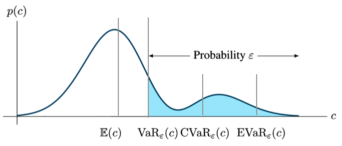
Entropic Value-at-Risk: Unfortunately, CVaR ignores the losses below the VaR threshold. EVaR is the tightest upper bound in the sense of Chernoff inequality for VaR and CVaR and its dual representation is associated with the relative entropy. In fact, it was shown in [8] that and are equal only if there are no losses () below the threshold. In addition, EVaR is a strictly monotone risk measure; whereas, CVaR is only monotone [7]. is given by
| (7) |
Similar to , for , corresponds to a risk-neutral case; whereas, corresponds to a risk-averse case. In fact, it was demonstrated in [6, Proposition 3.2] that .
III Problem Formulation
In the past two decades, coherent risk and dynamic risk measures have been developed and used in microeconomics and mathematical finance fields [49]. Generally speaking, risk-averse decision making is concerned with the behavior of agents, e.g. consumers and investors, who, when exposed to uncertainty, attempt to lower that uncertainty. The agents may avoid situations with unknown payoffs, in favor of situations with payoffs that are more predictable.
The core idea in risk-averse planning is to replace the conventional risk-neutral conditional expectation of the cumulative cost objectives with the more general coherent risk measures. In path planning scenarios, in particular, we will show in our numerical experiments that considering coherent risk measures will lead to significantly more robustness to environment uncertainty and collisions leading to mission failures.
In addition to total cost risk-aversity, an agent is often subject to constraints, e.g. fuel, communication, or energy budgets [27]. These constraints can also represent mission objectives, e.g. explore an area or reach a goal.
Consider a stationary controlled Markov process , (an MDP or a POMDP) with initial probability distribution , wherein policies, transition probabilities, and cost functions do not depend explicitly on time. Each policy leads to cost sequences , and , , . We define the dynamic risk of evaluating the -discounted cost of a policy as
| (8) |
and the -discounted dynamic risk constraints of executing policy as
| (9) |
where is defined in equation (4), , and , , are given constants. We assume that and , , are non-negative and upper-bounded. For a discount factor , an initial condition , and a policy , we infer from [41, Theorem 3] that both and are well-defined (bounded), if and are bounded.
In this work, we are interested in addressing the following problem:
Problem 1.
We call a controlled Markov process with the “nested” objective (8) and constraints (9) a constrained risk-averse Markov process.
For MDPs, [17, 33] show that such coherent risk measure objectives can account for modeling errors and parametric uncertainties. We can also interpret Problem 1 as designing policies that minimize the accrued costs in a risk-averse sense and at the same time ensuring that the system constraints, e.g., fuel constraints, are not violated even in the rare but costly scenarios.
Note that in Problem 1 both the objective function and the constraints are in general non-differentiable and non-convex in policy (with the exception of total expected cost as the coherent risk measure [9]). Therefore, finding optimal policies in general may be hopeless. Instead, we find sub-optimal polices by taking advantage of a Lagrangian formulation and then using an optimization form of Bellman’s equations.
Next, we show that the constrained risk-averse problem is equivalent to a non-constrained inf-sup risk-averse problem thanks to the Lagrangian method.
Proposition 1.
Let be the value of Problem 1 for a given initial distribution and discount factor . Then, (i) the value function satisfies
| (11) |
where
| (12) |
is the Lagrangian function.
(ii) Furthermore, a policy is optimal for Problem 1, if and only if .
Proof.
(i) If for some Problem 1 is not feasible, then . In fact, if the th constraint is not satisfied, i.e., , we can achieve the latter supremum by choosing , while keeping the rest of s constant or zero. If Problem 1 is feasible for some , then the supremum is achieved by setting . Hence, and
which implies (i).
(ii) If is optimal, then, from (11), we have
Conversely, if for some , then from (11), we have . Hence, is the optimal policy. ∎
IV Constrained Risk-Averse MDPs
At any time , the value of is -measurable and is allowed to depend on the entire history of the process and we cannot expect to obtain a Markov optimal policy [34, 11]. In order to obtain Markov policies, we need the following property [41].
Definition 4 (Markov Risk Measure).
Let such that and A one-step conditional risk measure is a Markov risk measure with respect to the controlled Markov process , , if there exist a risk transition mapping such that for all and , we have
| (13) |
where is called the controlled kernel.
In fact, if is a coherent risk measure, also satisfies the properties of a coherent risk measure (Definition 3). In this paper, since we are concerned with MDPs, the controlled kernel is simply the transition function .
Assumption 1.
The one-step coherent risk measure is a Markov risk measure.
The simplest case of the risk transition mapping is in the conditional expectation case , i.e.,
| (14) |
Note that in the total discounted expectation case is a linear function in rather than a convex function, which is the case for a general coherent risk measures. For example, for the CVaR risk measure, the Markov risk transition mapping is given by
where is a convex function in .
If is a coherent, Markov risk measure, then the Markov policies are sufficient to ensure optimality [41].
In the next result, we show that we can find a lower bound to the solution to Problem 1 via solving an optimization problem.
Theorem 1.
Proof.
From Proposition 1, we have know that (11) holds. Hence, we have
| (17) |
wherein the fourth, fifth, and sixth inequalities above we used the positive homogeneity property of , sub-additivity property of , and the minimax inequality respectively. Since does not depend on , to find the solution the infimum it suffices to find the solution to
where . The value to the above optimization can be obtained by solving the following Bellman equation [41, Theorem 4]
Next, we show that the solution to the above Bellman equation can be alternatively obtained by solving the convex optimization
| subject to | ||||
| (18) |
Define
and for all . From [41, Lemma 1], we infer that and are non-decreasing; i.e., for , we have and . Therefore, if , then . By repeated application of , we obtain
Any feasible solution to (IV) must satisfy and hence must satisfy . Thus, given that all entries of are positive, is the optimal solution to (IV). Substituting (IV) back in the last inequality in (IV) yields the result. ∎
Once the values of and are found by solving optimization problem (1), we can find the policy as
| (19) |
One interesting observation is that if the coherent risk measure is the total discounted expectation, then Theorem 1 is consistent with the classical result by [9] on constrained MDPs.
Corollary 1.
Proof.
From the derivation in (IV), we observe the two inequalities are from the application of (a) the sub-additivity property of and (b) the max-min inequality. Next, we show that in the case of total expectation both of these properties lead to an equality.
(a) Sub-additivity property of : for total expectation, we have
Thus, equality holds.
(b) Max-min inequality: in the case, both the objective function and the constraints are linear in the decision variables and . Therefore, the sixth line in (IV) reads as
| (20) |
Since the expression inside parantheses above is convex in ( is linear in the policy) and concave (linear) in . From Minimax Theorem [20], we have that the following equality holds
In [4], we presented a method based on difference convex programs to solve (1), when is an arbitrary coherent risk measure and we described the specific structure of the optimization problem for conditional expectation, CVaR, and EVaR. In fact, it was shown that (1) can be written in a standard DCP format as
| subject to | ||||
| (21) |
Optimization problem (IV) is a standard DCP [25]. DCPs arise in many applications, such as feature selection in machine learning [29] and inverse covariance estimation in statistics [48]. Although DCPs can be solved globally [25], e.g. using branch and bound algorithms [28], a locally optimal solution can be obtained based on techniques of nonlinear optimization [13] more efficiently. In particular, in this work, we use a variant of the convex-concave procedure [30, 43], wherein the concave terms are replaced by a convex upper bound and solved. In fact, the disciplined convex-concave programming (DCCP) [43] technique linearizes DCP problems into a (disciplined) convex program (carried out automatically via the DCCP Python package [43]), which is then converted into an equivalent cone program by replacing each function with its graph implementation. Then, the cone program can be solved readily by available convex programming solvers, such as CVXPY [18].
V Constrained Risk-Averse POMDPs
Next, we show that, in the case of POMDPs, we can find a lower bound to the solution to Problem 1 via solving an infinite-dimensional optimization problem. Note that a POMDP is equivalent to a belief MDP , , where is defined in (2).
Theorem 2.
Proof.
Note that a POMDP can be represented as an MDP over the belief states (2) with initial distribution (1). Hence, a POMDP is a controlled Markov process with states , where the controlled belief transition probability is described as
with
The rest of the proof follows the same footsteps on Theorem 1 over the belief MDP with as defined above. ∎
Unfortunately, since and hence , optimization (2) is infinite-dimensional and we cannot solve it efficiently.
If the one-step coherent risk measure is the total discounted expectation, we can show that optimization problem (2) simplifies to an infinite-dimensional linear program and equality holds in (23). This can be proved following the same lines as the proof of Corollary 1 but for the belief MDP. Hence, Theorem 2 also provides an optimization based solution to the constrained POMDP problem.
V-A Risk-Averse FSC Synthesis via Policy Iteration
In order to synthesize risk-averse FSCs, we employ a policy iteration algorithm. Policy iteration incrementally improves a controller by alternating between two steps: Policy Evaluation (computing value functions by fixing the policy) and Policy Improvement (computing the policy by fixing the value functions), until convergence to a satisfactory policy [12]. For a risk-averse POMDP, policy evaluation can be carried out by solving (2). However, as mentioned earlier, (2) is difficult to use directly as it must be computed at each (continuous) belief state in the belief space, which is uncountably infinite.
In the following, we show that if instead of considering policies with infinite-memory, we search over finite-memory policies, then we can find suboptimal solutions to Problem 1 that lower-bound . To this end, we consider stochastic but finite-memory controllers as described in Section II.C.
Closing the loop around a POMDP with an FSC induces a Markov chain. The global Markov chain (or simply , where the stochastic finite state controller and the POMDP are clear from the context) with execution . The probability of initial global state is
The state transition probability, , is given by
V-B Risk Value Function Computation
Under an FSC, the POMDP is transformed into a Markov chain with design probability distributions and . The closed-loop Markov chain is a controlled Markov process with , . In this setting, the total risk functional (8) becomes a function of and FSC , i.e.,
| (24) |
where s and s are drawn from the probability distribution . The constraint functionals , can also be defined similarly.
Let be the value of Problem 1 under a FSC . Then, it is evident that , since FSCs restrict the search space of the policy . That is, they can only be as good as the (infinite-dimensional) belief-based policy as (infinite-memory).
Risk Value Function Optimization: For POMDPs controlled by stochastic finite state controllers, the dynamic program is developed in the global state space . From Theorem 1, we see that for a given FSC, , and POMDP , the value function can be computed by solving the following finite dimensional optimization
| subject to | ||||
| (25) |
where and . Then, the solution satisfies
| (26) |
Note that since is a coherent, Markov risk measure (Assumption 1), is convex (because is also a coherent risk measure). In fact, optimization problem (V-B) is indeed a DCP in the form of (IV), where we should replace with and set , , , , and .
The above optimization is in standard DCP form because and are convex (linear) functions of and , , and are convex functions in .
Solving (IV) gives a set of value functions . In the next section, we discuss how to use the solutions from this DCP in our proposed policy iteration algorithm to sequentially improve the FSC parameters .
V-C I-States Improvement
Let denote the vectorized in . We say that an I-state is improved, if the tunable FSC parameters associated with that I-state can be adjusted so that increases.
To begin with, we compute the initial I-state by finding the best valued I-state for a given initial belief, i.e., , where
After this initialization, we search for FSC parameters that result in an improvement.
I-state Improvement Optimization: Given value functions for all and and Lagrangian parameters , for every I-state , we can find FSC parameters that result in an improvement by solving the following optimization
| subject to | |||
| Improvement Constraint: | |||
| Probability Constraints: | |||
| (27) |
Note that the above optimization searches for values that improve the I-state value vector by maximizing the auxiliary decision variable .
Optimization problem (V-C) is in general non-convex. This can be inferred from the fact that, although the first term in the r.h.s. of (V-B) is linear in , its convexity or concavity is not clear in the term for a general coherent risk measure. Fortunately, we can prove the following result.
Proposition 2.
Proof.
We present different forms of the Improvement Constraint in (V-C) for different risk measures. Note that the rest of the constraints and the cost function are linear in the decision variables and . The Improvement Constraint in (V-C) is linear in . However, its convexity or concavity in changes depending on the risk measure one considers. We recall from the previous section that in the Policy Evaluation step, the quantities for and (for conditional expectation, CVaR, and EVaR measures) and for (CVaR and EVaR measures) are calculated and therefore fixed here.
For conditional expectation, the Improvement Constraint alters to
| (28) |
Substituting the expression for , i.e.,
and , i.e.,
we obtain
| (29) |
The above expression is linear in as well as . Hence, I-State Improvement Optimization becomes a linear program for conditional expectation risk measure.
Based on a similar construction, for CVaR measure, the Improvement Constraint changes to
| (30) |
After substituting the term for , we obtain
| (31) |
| subject to | |||
| Improvement Constraint: | |||
| (32a) | |||
| Probability Constraints: | |||
| (32b) | |||
Furthermore, for fixed , , and , the above inequality is linear in and . Hence, (31) becomes a linear constraint rendering (V-C) a linear program (maximizing a linear objective subject to linear constraints), i.e., optimization problem (32).
For the EVaR measure, the Improvement Constraint is given by
| (33) |
Substituting the expression for , i.e.,
we obtain
| (34) |
| subject to | |||
| Improvement Constraint: | |||
| (35a) | |||
| Probability Constraints: | |||
| (35b) | |||
In the above inequality, the first term on the right-hand side of the is linear in and the second term on the right-hand side (logarithm term) is concave in (convex if all terms are moved to the left side, since is convex in ). Therefore, (34) becomes a convex constraint rendering (V-C) a convex optimization problem (maximizing a linear objective subject to linear and convex constraints) for EVaR measures. That is, the I-State Improvement Optimization takes the convex optimization form of (35). ∎
V-D Policy Iteration Algorithm
Algorithm 1 outlines the main steps in the proposed policy iteration method for the constrained risk-averse FSC synthesis. The algorithm has two distinct parts. First, for fixed parameters of the FSC (), policy evaluation is carried out, in which and are computed using DCP (V-B) (Steps 2, 10 and 18). Second, after evaluating the current value functions and the Lagrange multipliers, an improvement is carried out either by changing the parameters of existing I-states via optimization (V-C), or if no new parameters can improve any I-state, then a fixed number of I-states are added to escape the local minima (Steps 14-17) based on the method proposed in [3, Section V.B].
VI Numerical Experiments
In this section, we evaluate the proposed methodology with numerical experiments. In addition to the traditional total expectation, we consider two other coherent risk measures, namely, CVaR and EVaR. All experiments were carried out on a MacBook Pro with 2.8 GHz Quad-Core Intel Core i5 and 16 GB of RAM. The resultant linear programs and DCPs were solved using CVXPY [18] with DCCP [43] add-on in Python.
VI-A Rover MDP Example Set Up
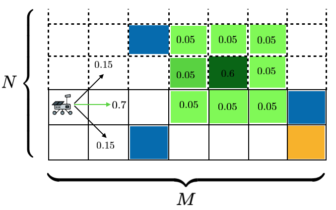
An agent (e.g. a rover) must autonomously navigate a 2-dimensional terrain map (e.g. Mars surface) represented by an grid with obstacles. The state space is given by The action set available to the robot is . The state transition probabilities for various cell types are shown for actions in Figure 2, i.e., the agent moves to the grid implied by the action with probability but can also move to any adjacent ones with probability. Partial observability arises because the rover cannot determine obstacle cell location from measurements directly. The observation space is Once at an adjacent cell to an obstacle, the rover can identify an actual obstacle position (dark green) with probability , and a distribution over the nearby cells (light green).
Hitting an obstacle incurs the immediate cost of , while the goal grid region has zero immediate cost. Any other grid has a cost of to represent fuel consumption. The discount factor is set to .
The objective is to compute a safe path that is fuel efficient, i.e., solving Problem 1. To this end, we consider total expectation, CVaR, and EVaR as the coherent risk measure.
Once a policy is calculated, as a robustness test, inspired by [17], we included a set of single grid obstacles that are perturbed in a random direction to one of the neighboring grid cells with probability to represent uncertainty in the terrain map. For each risk measure, we run Monte Carlo simulations with the calculated policies and count failure rates, i.e., the number of times a collision has occurred during a run.
VI-B MDP Results
To evaluate the technique discussed in Section IV, we assume that there is no partial observation. In our experiments, we consider four grid-world sizes of , , , and corresponding to , , , and states, respectively. For each grid-world, we randomly allocate 25% of the grids to obstacles, including 3, 6, 9, and 12 uncertain (single-cell) obstacles for the , , , and grids, respectively. In each case, we solve DCP (1) (linear program in the case of total expectation) with constraints and variables (the risk value functions ’s, Langrangian coefficient , and for CVaR and EVaR). In these experiments, we set for CVaR and EVaR coherent risk measures to represent risk-averse policies. The fuel budget (constraint bound ) was set to 50, 10, 200, and 600 for the , , , and grid-worlds, respectively. The initial condition was chosen as , i.e., the agent starts at the second left most grid at the bottom.
A summary of our numerical experiments is provided in Table 1. Note the computed values of Problem 1 satisfy , which is consistent with that fact that EVaR is a more conservative coherent risk measure than CVaR [6].
| Total Time [s] | # U.O. | F.R. | ||
| 9.12 | 0.8 | 3 | 11% | |
| 12.53 | 0.9 | 6 | 23% | |
| 19.93 | 1.7 | 9 | 33% | |
| 27.30 | 2.4 | 12 | 41% | |
| 12.04 | 5.8 | 3 | 8% | |
| 14.83 | 9.3 | 6 | 18% | |
| 20.19 | 10.34 | 9 | 19% | |
| 34.95 | 14.2 | 12 | 32% | |
| 14.45 | 6.2 | 3 | 3% | |
| 17.82 | 9.0 | 6 | 5% | |
| 25.63 | 11.1 | 9 | 13% | |
| 44.83 | 15.25 | 12 | 22% | |
| 14.53 | 4.8 | 3 | 4% | |
| 16.36 | 8.8 | 6 | 11% | |
| 29.89 | 10.5 | 9 | 15% | |
| 54.13 | 14.99 | 12 | 12% | |
| 18.03 | 5.8 | 3 | 1% | |
| 21.10 | 8.7 | 6 | 3% | |
| 24.08 | 10.2 | 9 | 7% | |
| 63.04 | 14.25 | 12 | 10% |
For total expectation coherent risk measure, the calculations took significantly less time, since they are the result of solving a set of linear programs. For CVaR and EVaR, a set of DCPs were solved. CVaR calculation was the most computationally involved. This observation is consistent with [7] were it was discussed that EVaR calculation is much more efficient than CVaR. Note that these calculations can be carried out offline for policy synthesis and then the policy can be applied for risk-averse robot path planning.
The table also outlines the failure ratios of each risk measure. In this case, EVaR outperformed both CVaR and total expectation in terms of robustness, which is consistent with the fact that EVaR is more conservative. In addition, these results imply that, although discounted total expectation is a measure of performance in high number of Monte Carlo simulations, it may not be practical to use it for mission-critical decision making under uncertainty scenarios. CVaR and especially EVaR seem to be a more reliable metric for performance in planning under uncertainty.
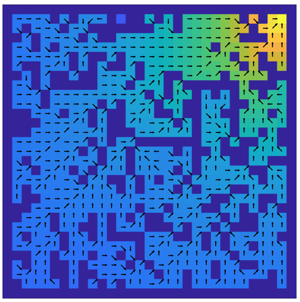
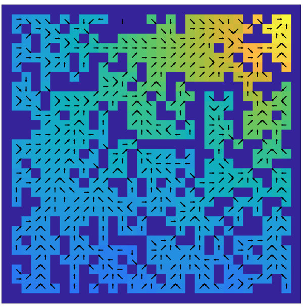
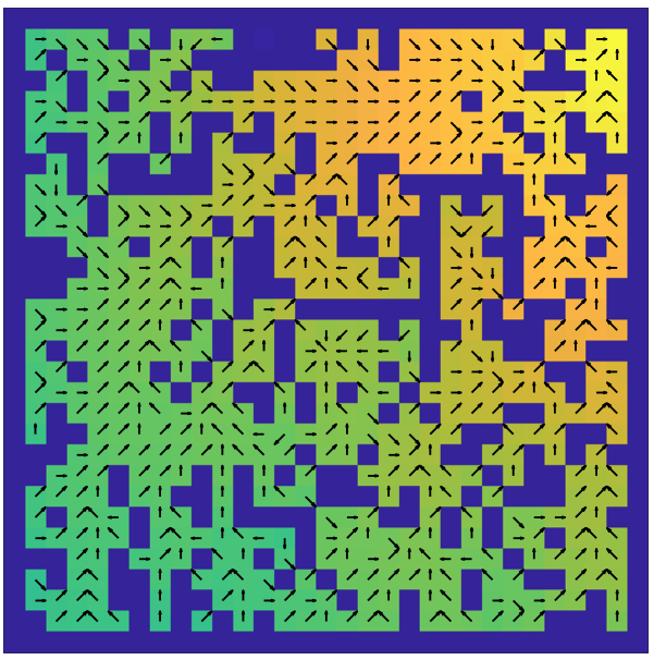
For the sake of illustrating the computed policies, Figure 3 depicts the results obtained from solving DCP (1) for a grid-world. The arrows on grids depict the (sub)optimal actions and the heat map indicates the values of Problem 1 for each grid state. Note that the values for EVaR are greater than those for CVaR and the values for CVaR are greater from those of total expectation. This is in accordance with the theory that [6]. In addition, by inspecting the computed actions in obstacle dense areas of the grid-world (for example, the middle right area), we infer that the actions in more risk-averse cases (especially, for EVaR) have a higher tendency to steer the agent away from the obstacles given the diagonal transition uncertainty as depicted in Figure 2; whereas, for total expectation, the actions are merely concerned about reaching the goal.
VI-C POMDP Results
In our experiments, we consider two grid-world sizes of and corresponding to and states, respectively. For each grid-world, we allocate 25% of the grid to obstacles, including 8, and 16 uncertain (single-cell) obstacles for the and grids, respectively. In each case, we run Algorithm 1 for risk-averse FSC synthesis with and a maximum number of 100 iterations were considered.
In these experiments, we set the confidence level for CVaR and EVaR coherent risk measures. The fuel budget (constraint bound ) was set to 50 and 200 for the and grid-worlds, respectively. The initial condition was chosen as , i.e., the agent starts at the right most grid at the bottom.
A summary of our numerical experiments is provided in Table 1. Note the computed values of Problem 1 satisfy [6].
| AIT [s] | # U.O. | F.R. | ||
| 10.53 | 0.2 | 3 | 15% | |
| 19.98 | 0.3 | 9 | 37% | |
| 11.02 | 2.9 | 3 | 9% | |
| 20.19 | 7.5 | 9 | 22% | |
| 16.53 | 3.1 | 3 | 4% | |
| 24.92 | 7.6 | 9 | 16% | |
| 15.02 | 3.3 | 3 | 5% | |
| 23.42 | 9.9 | 9 | 11% | |
| 19.62 | 3.9 | 3 | 2% | |
| 29.36 | 9.7 | 9 | 6% |
For total expectation coherent risk measure, the calculations took significantly less time, since they are the result of solving a set of linear programs. For CVaR and EVaR, a set of DCPs were solved in the Risk Value Function Computation step. In the I-State Improvement step, a set of linear programs were solved for CVaR and convex optimizations for EVaR. Hence, EVaR calculation was the most computationally involved in this case. Note that these calculations can be carried out offline for policy synthesis and then the policy can be applied for risk-averse robot path planning.
The table also outlines the failure ratios of each risk measure. In this case, EVaR outperformed both CVaR and total expectation in terms of robustness, tallying with the fact that EVaR is conservative. In addition, these results suggest that, although discounted total expectation is a measure of performance in high number of Monte Carlo simulations, it may not be practical to use it for real-world planning under uncertainty scenarios. CVaR and especially EVaR seem to be a more reliable metric for performance in planning under uncertainty.
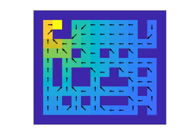

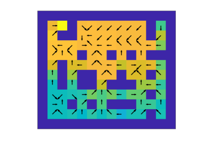
For the sake of illustrating the computed policies, Figure 3 depicts the results obtained from solving DCP (1) for a grid-world. The arrows on grids depict the (sub)optimal actions and the heat map indicates the values of Problem 1 for each grid state. Note that the values for EVaR are greater than those for CVaR and the values for CVaR are greater from those of total expectation. This is in accordance with the theory that [6].
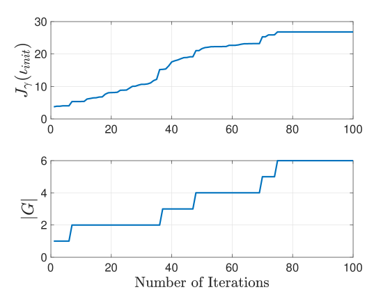
Moreover, for the gridworld with EVaR coherent risk measure, Figure 2 depicts the evolution of the number of FSC I-states and the lower bound on the optimal value of Problem 1, , with respect to the iteration number of Algorithm 1. We can see that as the number of I-states increase, the lower bound is improved.
VII Conclusions and Future Research
We proposed an optimization-based method for designing policies for MDPs and POMDPs with coherent risk measure objectives and constraints. We showed that such value function optimizations are in the form of DCPs. In the case of POMDPs, we proposed a policy iteration method for finding sub-optimal FSCs that lower-bound the constrained risk-averse problem and we demonstrated that dependent on the coherent risk measure of interest the policy search can be carried out via a linear program or a convex optimization. Numerical experiments were provided to show the efficacy of our approach. In particular, we showed that considering coherent risk measures lead to significantly lower collision rates in Monte Carlo simulations in navigation problems.
In this work, we focused on discounted infinite horizon risk-averse problems. Future work will explore other cost criteria [14]. The interested reader is referred to our preliminary results on total cost risk-averse MDPs [1], where in Bellman’s equations for the risk-averse stochastic shortest path problem are derived. Expanding on the latter work, we will also explore high-level mission specifications in terms of temporal logic formulas for risk-averse MDPs and POMDPs [5, 40]. Another area for more research is concerned with receding-horizon motion planning under uncertainty with coherent risk constraints [19, 24], with particular application in robot exploration in unstructured subterranean environments [21] (also see works on receding horizon path planning where the coherent risk measure is in the total cost [45, 44] rather than the collision avoidance constraint).
Acknowledgment
M. Ahmadi acknowledges stimulating discussions with Dr. Masahiro Ono at NASA Jet Propulsion Laboratory and Prof. Marco Pavone at Nvidia Research-Stanford University.
References
- [1] M. Ahmadi, A. Dixit, J. W. Burdick, and A. D. Ames. Risk-averse stochastic shortest path planning. arXiv preprint arXiv:2103.14727, 2021.
- [2] M. Ahmadi, N. Jansen, B. Wu, and U. Topcu. Control theory meets POMDPs: A hybrid systems approach. IEEE Transactions on Automatic Control, 2020.
- [3] M. Ahmadi, M. Ono, M. D. Ingham, R. M. Murray, and A. D. Ames. Risk-averse planning under uncertainty. In 2020 American Control Conference (ACC), pages 3305–3312. IEEE, 2020.
- [4] M. Ahmadi, U. Rosolia, M. Ingham, R. Murray, and A. Ames. Constrained risk-averse Markov decision processes. In 35th AAAI Conference on Artificial Intelligence, 2021.
- [5] M. Ahmadi, R. Sharan, and J. W. Burdick. Stochastic finite state control of POMDPs with LTL specifications. arXiv preprint arXiv:2001.07679, 2020.
- [6] A. Ahmadi-Javid. Entropic value-at-risk: A new coherent risk measure. Journal of Optimization Theory and Applications, 155(3):1105–1123, 2012.
- [7] A. Ahmadi-Javid and M. Fallah-Tafti. Portfolio optimization with entropic value-at-risk. European Journal of Operational Research, 279(1):225–241, 2019.
- [8] A. Ahmadi-Javid and A. Pichler. An analytical study of norms and banach spaces induced by the entropic value-at-risk. Mathematics and Financial Economics, 11(4):527–550, 2017.
- [9] E. Altman. Constrained Markov decision processes, volume 7. CRC Press, 1999.
- [10] P. Artzner, F. Delbaen, J. Eber, and D. Heath. Coherent measures of risk. Mathematical finance, 9(3):203–228, 1999.
- [11] N. Bäuerle and J. Ott. Markov decision processes with average-value-at-risk criteria. Mathematical Methods of Operations Research, 74(3):361–379, 2011.
- [12] Dimitri P Bertsekas. Dynamic programming and stochastic control. Number 10. Academic Press, 1976.
- [13] D.P. Bertsekas. Nonlinear Programming. Athena Scientific, 1999.
- [14] S. Carpin, Y. Chow, and M. Pavone. Risk aversion in finite Markov Decision Processes using total cost criteria and average value at risk. In 2016 ieee international conference on robotics and automation (icra), pages 335–342. IEEE, 2016.
- [15] Anthony R. Cassandra, Leslie Pack Kaelbling, and Michael L. Littman. Acting optimally in partially observable stochastic domains. In AAAI, pages 1023–1028, 1994.
- [16] Y. Chow and M. Ghavamzadeh. Algorithms for cvar optimization in mdps. In Advances in neural information processing systems, pages 3509–3517, 2014.
- [17] Y. Chow, A. Tamar, S. Mannor, and M. Pavone. Risk-sensitive and robust decision-making: a cvar optimization approach. In Advances in Neural Information Processing Systems, pages 1522–1530, 2015.
- [18] S. Diamond and S. Boyd. CVXPY: A Python-embedded modeling language for convex optimization. Journal of Machine Learning Research, 17(83):1–5, 2016.
- [19] A. Dixit, M. Ahmadi, and J. W. Burdick. Risk-sensitive motion planning using entropic value-at-risk. In European Control Conference, 2021.
- [20] D. Du and P. M. Pardalos. Minimax and applications, volume 4. Springer Science & Business Media, 2013.
- [21] D. D. Fan, K. Otsu, Y. Kubo, A. Dixit, J. Burdick, and A. Agha-Mohammadi. STEP: Stochastic traversability evaluation and planning for safe off-road navigation. arXiv preprint arXiv:2103.02828, 2021.
- [22] J. Fan and A. Ruszczyński. Process-based risk measures and risk-averse control of discrete-time systems. Mathematical Programming, pages 1–28, 2018.
- [23] J. Fan and A. Ruszczyński. Risk measurement and risk-averse control of partially observable discrete-time markov systems. Mathematical Methods of Operations Research, 88(2):161–184, 2018.
- [24] A. Hakobyan, Gyeong C. Kim, and I. Yang. Risk-aware motion planning and control using CVaR-constrained optimization. IEEE Robotics and Automation Letters, 4(4):3924–3931, 2019.
- [25] R. Horst and N. V. Thoai. DC programming: overview. Journal of Optimization Theory and Applications, 103(1):1–43, 1999.
- [26] V. Krishnamurthy. Partially observed Markov decision processes. Cambridge University Press, 2016.
- [27] V. Krishnamurthy and S. Bhatt. Sequential Detection of Market Shocks With Risk-Averse CVaR Social Sensors. IEEE Journal of Selected Topics in Signal Processing, 10(6):1061–1072, 2016.
- [28] E. L. Lawler and D. E. Wood. Branch-and-bound methods: A survey. Operations research, 14(4):699–719, 1966.
- [29] H. A. Le Thi, H. M. Le, T. P. Dinh, et al. A dc programming approach for feature selection in support vector machines learning. Advances in Data Analysis and Classification, 2(3):259–278, 2008.
- [30] T. Lipp and S. Boyd. Variations and extension of the convex–concave procedure. Optimization and Engineering, 17(2):263–287, 2016.
- [31] O. Madani, S. Hanks, and A. Condon. On the undecidability of probabilistic planning and related stochastic optimization problems. Artificial Intelligence, 147(1):5 – 34, 2003.
- [32] A. Majumdar and M. Pavone. How should a robot assess risk? towards an axiomatic theory of risk in robotics. In Robotics Research, pages 75–84. Springer, 2020.
- [33] T. Osogami. Robustness and risk-sensitivity in markov decision processes. In Advances in Neural Information Processing Systems, pages 233–241, 2012.
- [34] Jonathan Theodor Ott. A Markov decision model for a surveillance application and risk-sensitive Markov decision processes. 2010.
- [35] G. C. Pflug and A. Pichler. Time-consistent decisions and temporal decomposition of coherent risk functionals. Mathematics of Operations Research, 41(2):682–699, 2016.
- [36] L. Prashanth. Policy gradients for CVaR-constrained MDPs. In International Conference on Algorithmic Learning Theory, pages 155–169. Springer, 2014.
- [37] Martin L. Puterman. Markov Decision Processes: Discrete Stochastic Dynamic Programming. John Wiley & Sons, Inc., New York, NY, USA, 1st edition, 1994.
- [38] R Tyrrell Rockafellar and Stanislav Uryasev. Conditional value-at-risk for general loss distributions. Journal of banking & finance, 26(7):1443–1471, 2002.
- [39] R Tyrrell Rockafellar, Stanislav Uryasev, et al. Optimization of conditional value-at-risk. Journal of risk, 2:21–42, 2000.
- [40] U. Rosolia, M. Ahmadi, R. M. Murray, and A. D. Ames. Time-optimal navigation in uncertain environments with high-level specifications. arXiv preprint arXiv:2103.01476, 2021.
- [41] A. Ruszczyński. Risk-averse dynamic programming for markov decision processes. Mathematical programming, 125(2):235–261, 2010.
- [42] A. Shapiro, D. Dentcheva, and A. Ruszczyński. Lectures on stochastic programming: modeling and theory. SIAM, 2014.
- [43] X. Shen, S. Diamond, Y. Gu, and S. Boyd. Disciplined convex-concave programming. In 2016 IEEE 55th Conference on Decision and Control (CDC), pages 1009–1014. IEEE, 2016.
- [44] S. Singh, Y. Chow, A. Majumdar, and M. Pavone. A framework for time-consistent, risk-sensitive model predictive control: Theory and algorithms. IEEE Transactions on Automatic Control, 2018.
- [45] P. Sopasakis, D. Herceg, A. Bemporad, and P. Patrinos. Risk-averse model predictive control. Automatica, 100:281–288, 2019.
- [46] A. Tamar, Y. Chow, M. Ghavamzadeh, and S. Mannor. Policy gradient for coherent risk measures. In Advances in Neural Information Processing Systems, pages 1468–1476, 2015.
- [47] A. Tamar, Y. Chow, M. Ghavamzadeh, and S. Mannor. Sequential decision making with coherent risk. IEEE Transactions on Automatic Control, 62(7):3323–3338, 2016.
- [48] J. Thai, T. Hunter, A. K. Akametalu, C. J. Tomlin, and A. M. Bayen. Inverse covariance estimation from data with missing values using the concave-convex procedure. In 53rd IEEE Conference on Decision and Control, pages 5736–5742. IEEE, 2014.
- [49] D. Vose. Risk analysis: a quantitative guide. John Wiley & Sons, 2008.
- [50] A. Wang, A. M Jasour, and B. Williams. Non-gaussian chance-constrained trajectory planning for autonomous vehicles under agent uncertainty. IEEE Robotics and Automation Letters, 2020.
- [51] Huan Xu and Shie Mannor. Distributionally robust markov decision processes. In Advances in Neural Information Processing Systems, volume 23, pages 2505–2513, 2010.