This paper was converted on www.awesomepapers.org from LaTeX by an anonymous user.
Want to know more? Visit the Converter page.

Risk Bounds for Mixture Density Estimation on Compact Domains via the hh-Lifted Kullback–Leibler Divergence

Mark Chiu Chong mark.chiuchong@gmail.com
School of Mathematics and Physics
The University of Queensland
St Lucia, QLD 4072, Australia
Hien Duy Nguyen hien@imi.kyushu-u.ac.jp
Institute of Mathematics for Industry
Kyushu University
Nishi Ward, Fukuoka 819-0395, Japan;
School of Computing, Engineering, and Mathematical Sciences
La Trobe University
Bundoora, VIC 3086, Australia;
TrungTin Nguyen trungtin.nguyen@uq.edu.au
School of Mathematics and Physics
The University of Queensland
St Lucia, QLD 4072, Australia
Abstract

We consider the problem of estimating probability density functions based on sample data, using a finite mixture of densities from some component class. To this end, we introduce the hh-lifted Kullback–Leibler (KL) divergence as a generalization of the standard KL divergence and a criterion for conducting risk minimization. Under a compact support assumption, we prove an 𝒪(1/n)\mathcal{O}(1/{\sqrt{n}}) bound on the expected estimation error when using the hh-lifted KL divergence, which extends the results of Rakhlin et al. (2005, ESAIM: Probability and Statistics, Vol. 9) and Li & Barron (1999, Advances in Neural Information Processing Systems, Vol. 12) to permit the risk bounding of density functions that are not strictly positive. We develop a procedure for the computation of the corresponding maximum hh-lifted likelihood estimators (hh-MLLEs) using the Majorization-Maximization framework and provide experimental results in support of our theoretical bounds.

1 Introduction

Let (Ω,𝔄,𝐏)\left(\Omega,\mathfrak{A},{\mathrm{\mathbf{P}}}\right) be an abstract probability space and let X:Ω𝒳X:\Omega\to\mathcal{X} be a random variable taking values in the measurable space (𝒳,𝔉)\left(\mathcal{X},\mathfrak{F}\right), where 𝒳\mathcal{X} is a compact metric space equipped with its Borel σ\sigma-algebra 𝔉\mathfrak{F}. Suppose that we observe an independent and identically distributed (i.i.d.) sample of random variables 𝐗n=(Xi)i[n]\mathbf{X}_{n}=\left(X_{i}\right)_{i\in\left[n\right]}, where [n]={1,,n}\left[n\right]=\left\{1,\ldots,n\right\}, and that each XiX_{i} arises from the same data generating process as XX, characterized by the probability measure FμF\ll\mu on (𝒳,𝔉)\left(\mathcal{X},\mathfrak{F}\right), with density function f=dF/dμf=\mathrm{d}F/\mathrm{d}\mu, for some σ\sigma-finite μ\mu. In this work, we are concerned with the estimating ff via a data dependent double-index sequence of estimators (fk,n)k,n\left(f_{k,n}\right)_{k,n\in\mathbb{N}}, where

fk,n𝒞k=cok(𝒫)={fk(;ψk)=j=1kπjφ(;θj)φ(;θj)𝒫,πj0,j[k],j=1kπj=1},\displaystyle f_{k,n}\in\mathcal{C}_{k}=\mathrm{co}_{k}\left(\mathcal{P}\right)=\left\{f_{k}\left(\cdot;\psi_{k}\right)=\sum_{j=1}^{k}\pi_{j}\varphi\left(\cdot;\theta_{j}\right)\mid\varphi\left(\cdot;\theta_{j}\right)\in\mathcal{P},\,\pi_{j}\geq 0,\,j\in\left[k\right],\sum_{j=1}^{k}\pi_{j}=1\right\},

for each k,nk,n\in\mathbb{N}, and where

𝒫={φ(;θ):𝒳0θΘd},\mathcal{P}=\left\{\varphi\left(\cdot;\theta\right):\mathcal{X}\rightarrow\mathbb{R}_{\geq 0}\mid\theta\in\Theta\subset\mathbb{R}^{d}\right\}, (1)

ψk=(π1,,πk,θ1,,θk)\psi_{k}=\left(\pi_{1},\dots,\pi_{k},\theta_{1},\dots,\theta_{k}\right), and dd\in\mathbb{N}. To ensure the measurability and existence of various optima, we shall assume that φ\varphi is Carathéodory in the sense that φ(;θ)\varphi\left(\cdot;\theta\right) is (𝒳,𝔉)\left(\mathcal{X},\mathfrak{F}\right)-measurable for each θΘ\theta\in\Theta, and φ(X;)\varphi\left(X;\cdot\right) is continuous for each X𝒳X\in\mathcal{X}.

In the definition above, we can identify the set 𝒞k=cok(𝒫)\mathcal{C}_{k}=\mathrm{co}_{k}\left(\mathcal{P}\right) as the set of density functions that can be written as a convex combination of kk elements of 𝒫\mathcal{P}, where 𝒫\mathcal{P} is often called the space of component density functions. We then interpret 𝒞k\mathcal{C}_{k} as the class of kk-component finite mixtures of densities of class 𝒫\mathcal{P}, as studied, for example, by McLachlan & Peel (2004); Nguyen et al. (2020; 2022b).

1.1 Risk bounds for mixture density estimation

We are particularly interested in oracle bounds of the form

𝐄{(f,fk,n)}(f,𝒞)ρ(k,n),{\mathrm{\mathbf{E}}}\left\{\ell\left(f,f_{k,n}\right)\right\}-\ell\left(f,\mathcal{C}\right)\leq\rho\left(k,n\right), (2)

where (p,q)(p,q)0\left(p,q\right)\mapsto\ell\left(p,q\right)\in\mathbb{R}_{\geq 0} is a loss function on pairs of density functions. We define the density-to-class loss

(f,𝒞)=infq𝒞(f,q),𝒞=cl(kcok(𝒫)),\ell\left(f,\mathcal{C}\right)=\inf_{q\in\mathcal{C}}\ell\left(f,q\right),\ \mathcal{C}=\mathrm{cl}\left(\bigcup_{k\in\mathbb{N}}\mathrm{co}_{k}\left(\mathcal{P}\right)\right),

where cl()\mathrm{cl}(\cdot) is the closure. Here, we identify (k,n)ρ(k,n)\left(k,n\right)\mapsto\rho\left(k,n\right) as a characterization of the rate at which the left-hand side of (2) converges to zero as kk and nn increase. Our present work follows the research of Li & Barron (1999), Rakhlin et al. (2005) and Klemelä (2007) (see also Klemelä 2009, Ch. 19). In Li & Barron (1999) and Rakhlin et al. (2005), the authors consider the case where (p,q)\ell\left(p,q\right) is taken to be the Kullback–Leibler (KL) divergence

KL(p||q)=plogpqdμ\mathrm{KL}\left(p\,||\,q\right)=\int p\log\frac{p}{q}\mathrm{d}\mu

and fk,n=fk(;ψk,n)f_{k,n}=f_{k}\left(\cdot;{\psi}_{k,n}\right) is a maximum likelihood estimator (MLE), where

ψk,nargmaxψk𝒮k×Θk1ni=1nlogfk(Xi;ψk),{\psi}_{k,n}\in\underset{\psi_{k}\in\mathcal{S}_{k}\times\Theta^{k}}{\operatorname*{arg\,max\,}}\frac{1}{n}\sum_{i=1}^{n}\log f_{k}\left(X_{i};\psi_{k}\right),

is a function of 𝐗n\mathbf{X}_{n}, with 𝒮k\mathcal{S}_{k} denoting the probability simplex in k\mathbb{R}^{k}.

Under the assumption that f,fkaf,f_{k}\geq a, for some a>0a>0 and each k[n]k\in\left[n\right] (i.e., strict positivity), Li & Barron (1999) obtained the bound

𝐄{KL(f||fk,n)}KL(f||𝒞)c11k+c2klog(c3n)n,{\mathrm{\mathbf{E}}}\left\{\mathrm{KL}\left(f\,||\,f_{k,n}\right)\right\}-\mathrm{KL}\left(f\,||\,\mathcal{C}\right)\leq c_{1}\frac{1}{k}+c_{2}\frac{k\log\left(c_{3}n\right)}{n},

for constants c1,c2,c3>0c_{1},c_{2},c_{3}>0, which was then improved by Rakhlin et al. (2005) who obtained the bound

𝐄{KL(f||fk,n)}KL(f||𝒞)c11k+c21n,{\mathrm{\mathbf{E}}}\left\{\mathrm{KL}\left(f\,||\,f_{k,n}\right)\right\}-\mathrm{KL}\left(f\,||\,\mathcal{C}\right)\leq c_{1}\frac{1}{k}+c_{2}\frac{1}{\sqrt{n}},

for constants c1,c2>0c_{1},c_{2}>0 (constants (cj)j(c_{j})_{j\in\mathbb{N}} are typically different between expressions).

Alternatively, Klemelä (2007) takes (p,q)\ell\left(p,q\right) to be the squared L2(μ)L_{2}\left(\mu\right) norm distance (i.e., the least-squares loss):

(p,q)=pq2,μ2,\ell\left(p,q\right)=\lVert p-q\rVert_{2,\mu}^{2},

where p2,μ2=𝒳|p|2dμ\lVert p\rVert_{2,\mu}^{2}=\int_{\mathcal{X}}\lvert p\rvert^{2}\mathrm{d}\mu, for each pL2(μ)p\in L_{2}\left(\mu\right), and choose fk,nf_{k,n} as minimizers of the L2(μ)L_{2}\left(\mu\right) empirical risk, i.e., fk,n=fk(;ψk,n)f_{k,n}=f_{k}\left(\cdot;{\psi}_{k,n}\right), where

ψk,nargminψk𝒮k×Θk2ni=1nfk(;ψk)+fk(;ψk)2,μ2.\psi_{k,n}\in\underset{\psi_{k}\in\mathcal{S}_{k}\times\Theta^{k}}{\operatorname*{arg\,min\,}}-\frac{2}{n}\sum_{i=1}^{n}f_{k}\left(\cdot;\psi_{k}\right)+\left\|f_{k}\left(\cdot;\psi_{k}\right)\right\|_{2,\mu}^{2}. (3)

Here, Klemelä (2007) establish the bound

𝐄ffk,n2,μ2infq𝒞fq2,μ2c11k+c21n,{\mathrm{\mathbf{E}}}\left\|f-{f}_{k,n}\right\|_{2,\mu}^{2}-\inf_{q\in\mathcal{C}}\left\|f-q\right\|_{2,\mu}^{2}\leq c_{1}\frac{1}{k}+c_{2}\frac{1}{\sqrt{n}},

c1,c2>0c_{1},c_{2}>0, without the lower bound assumption on f,fkf,f_{k} above, even permitting 𝒳\mathcal{X} to be unbounded. Via the main results of Naito & Eguchi (2013), the bound above can be generalized to the UU-divergences, which includes the special L2(μ)L_{2}(\mu) norm distance as a special case.

On the one hand, the sequence of MLEs required for the results of Li & Barron (1999) and Rakhlin et al. (2005) are typically computable, for example, via the usual expectation–maximization approach (cf. McLachlan & Peel 2004, Ch. 2). This contrasts with the computation of least-squares density estimators of form (3), which requires evaluations of the typically intractable integral expressions fk(;ψk)22\left\|f_{k}\left(\cdot;\psi_{k}\right)\right\|_{2}^{2}. However, the least-squares approach of Klemelä (2007) permits the analysis using families 𝒫\mathcal{P} of usual interest, such as normal distributions and beta distributions, the latter of which being compactly supported but having densities that cannot be bounded away from zero without restrictions, and thus do not satisfy the regularity conditions of Li & Barron (1999) and Rakhlin et al. (2005).

1.2 Main contributions

We propose the following hh-lifted KL divergence, as a generalization of the standard KL divergence to address the computationally tractable estimation of density functions which do not satisfy the regularity conditions of Li & Barron (1999) and Rakhlin et al. (2005). The use of the hh-lifted KL divergence has the possibility to advance theories based on the standard KL divergence in statistical machine learning. To this end, let h:𝒳0h:\mathcal{X}\rightarrow\mathbb{R}_{\geq 0} be a function in L1(μ)L_{1}(\mu), and define the hh-lifted KL divergence by:

KLh(p||q)=𝒳{p+h}logp+hq+hdμ.\mathrm{KL}_{h}\left(p\,||\,q\right)=\int_{\mathcal{X}}\left\{p+h\right\}\log\frac{p+h}{q+h}\mathrm{d}\mu. (4)

In the sequel, we shall show that KLh\mathrm{KL}_{h} is a Bregman divergence on the space of probability density functions, as per Csiszár (1995).

Assume that hh is a probability density function, and let 𝐘n=(Yi)i[n]\mathbf{Y}_{n}=\left(Y_{i}\right)_{i\in\left[n\right]} be a an i.i.d. sample, independent of 𝐗n\mathbf{X}_{n}, where each Yi:Ω𝒳Y_{i}:\Omega\rightarrow\mathcal{X} is a random variable with probability measure on (𝒳,𝔉)(\mathcal{X},\mathfrak{F}), characterized by the density hh with respect to μ\mu. Then, for each kk and nn, let fk,nf_{k,n} be defined via the maximum hh-lifted likelihood estimator (hh-MLLE; see Appendix B for further discussion) fk,n=fk(;ψk,n)f_{k,n}=f_{k}\left(\cdot;{\psi}_{k,n}\right), where

ψk,nargmaxψk𝒮k×Θk1ni=1n(log{fk(Xi;ψk)+h(Xi)}+log{fk(Yi;ψk)+h(Yi)}).{\psi}_{k,n}\in\underset{\psi_{k}\in\mathcal{S}_{k}\times\Theta^{k}}{\operatorname*{arg\,max\,}}~{}\frac{1}{n}\sum_{i=1}^{n}\left(\log\left\{f_{k}\left(X_{i};\psi_{k}\right)+h\left(X_{i}\right)\right\}+\log\left\{f_{k}\left(Y_{i};\psi_{k}\right)+h\left(Y_{i}\right)\right\}\right). (5)

The primary aim of this work is to show that

𝐄{KLh(f||fk,n)}KLh(f||𝒞)c11k+c21n{\mathrm{\mathbf{E}}}\left\{\mathrm{KL}_{h}\left(f\,||\,f_{k,n}\right)\right\}-\mathrm{KL}_{h}\left(f\,||\,\mathcal{C}\right)\leq c_{1}\frac{1}{k}+c_{2}\frac{1}{\sqrt{n}} (6)

for some constants c1,c2>0c_{1},c_{2}>0, without requiring the strict positivity assumption that f,fka>0f,f_{k}\geq a>0.

This result is a compromise between the works of Li & Barron (1999) and Rakhlin et al. (2005), and Klemelä (2007), as it applies to a broader space of component densities 𝒫\mathcal{P}, and because the required hh-MLLEs (5) can be efficiently computed via minorization–maximization (MM) algorithms (see e.g., Lange 2016). We shall discuss this assertion in Section 4.

1.3 Relevant literature

Our work largely follows the approach of Li & Barron (1999), which was extended upon by Rakhlin et al. (2005) and Klemelä (2007). All three texts use approaches based on the availability of greedy algorithms for maximizing convex functions with convex functional domains. In this work, we shall make use of the proof techniques of Zhang (2003). Related results in this direction can be found in DeVore & Temlyakov (2016) and Temlyakov (2016). Making the same boundedness assumption as Rakhlin et al. (2005), Dalalyan & Sebbar (2018) obtain refined oracle inequalities under the additional assumption that the class 𝒫\mathcal{P} is finite. Numerical implementations of greedy algorithms for estimating finite mixtures of Gaussian densities were studied by Vlassis & Likas (2002) and Verbeek et al. (2003).

The hh-MLLE as an optimization objective can be compared to other similar modified likelihood estimators, such as the LqL_{q} likelihood of Ferrari & Yang (2010) and Qin & Priebe (2013), the β\beta-likelihood of Basu et al. (1998) and Fujisawa & Eguchi (2006), penalized likelihood estimators, such as maximum a posteriori estimators of Bayesian models, or ff-separable Bregman distortion measures of Kobayashi & Watanabe (2024; 2021).

The practical computation of the hh-MLLEs, (5), is made possible via the MM algorithm framework of Lange (2016), see also Hunter & Lange (2004), Wu & Lange (2010), and Nguyen (2017) for further details. Such algorithms have well-studied global convergence properties and can be modified for mini-batch and stochastic settings (see, e.g., Razaviyayn et al., 2013 and Nguyen et al., 2022a).

A related and popular setting of investigations is that of model selection, where the objects of interest are single-index sequences (fkn,n)n\left(f_{k_{n},n}\right)_{n\in\mathbb{N}}, and where the aim is to obtain finite-sample bounds for losses of the form (fkn,n,f)\ell\left(f_{k_{n},n},f\right), where each knk_{n}\in\mathbb{N} is a data dependent function, often obtained by optimizing some penalized loss criterion, as described in Massart (2007), Koltchinskii (2011, Ch. 6), and Giraud (2021, Ch. 2). In the context of finite mixtures, examples of such analyses can be found in the works of Maugis & Michel (2011) and Maugis-Rabusseau & Michel (2013). A comprehensive bibliography of model selection results for finite mixtures and related statistical models can be found in Nguyen et al. (2022c).

1.4 Organization of paper

The manuscript is organized as follows. In Section 2, we formally define the hh-lifted KL divergence as a Bregman divergence and establish several of its properties. In Section 3, we present new risk bounds for the hh-lifted KL divergence of the form (2). In Section 4, we discuss the computation of the hh-lifted likelihood estimator in the form of (5), followed by empirical results illustrating the convergence of (2) with respect to both kk and nn. Additional insights and technical results are provided in the Appendices at the end of the manuscript.

2 The hh-lifted KL divergence and its properties

In this section we formally define the hh-lifted KL divergence on the space of density functions and establish some of its properties.

Definition 1 (hh-lifted KL divergence).

Let f,gf,g, and hh be probability density functions on the space 𝒳\mathcal{X}, where h>0h>0. The hh-lifted KL divergence from gg to ff is defined as follows:

KLh(f||g)=𝒳{f+h}logf+hg+hdμ=𝐄f{logf+hg+h}+𝐄h{logf+hg+h}.\mathrm{KL}_{h}\left(f\,||\,g\right)=\int_{\mathcal{X}}\left\{f+h\right\}\log\frac{f+h}{g+h}\mathrm{d}\mu={\operatorname*{{\mathrm{\mathbf{E}}}}}_{f}\left\{\log\frac{f+h}{g+h}\right\}+{\operatorname*{{\mathrm{\mathbf{E}}}}}_{h}\left\{\log\frac{f+h}{g+h}\right\}.

2.1 KLh\textrm{KL}_{h} as a Bregman divergence

Let ϕ:\phi:\mathcal{I}\to\operatorname*{\mathbb{R}}, =(0,)\mathcal{I}=(0,\infty) be a strictly convex function that is continuously differentiable. The Bregman divergence between scalars dϕ:×0d_{\phi}:\mathcal{I}\times\mathcal{I}\to\mathbb{R}_{\geq 0} generated by the function ϕ\phi is given by:

dϕ(p,q)=ϕ(p)ϕ(q)ϕ(q)(pq),d_{\phi}(p,q)=\phi(p)-\phi(q)-\phi^{\prime}(q)(p-q),

where ϕ(q)\phi^{\prime}(q) denotes the derivative of ϕ\phi at qq.

Bregman divergences possess several useful properties, including the following list:

  1. 1.

    Non-negativity: dϕ(p,q)0d_{\phi}(p,q)\geq 0 for all p,qp,q\in\mathcal{I} with equality if and only if p=qp=q;

  2. 2.

    Asymmetry: dϕ(p,q)dϕ(q,p)d_{\phi}(p,q)\neq d_{\phi}(q,p) in general;

  3. 3.

    Convexity: dϕ(p,q)d_{\phi}(p,q) is convex in pp for every fixed qq\in\mathcal{I}.

  4. 4.

    Linearity: dc1ϕ1+c2ϕ2(p,q)=c1dϕ1(p,q)+c2dϕ2(p,q)d_{c_{1}\phi_{1}+c_{2}\phi_{2}}(p,q)=c_{1}d_{\phi_{1}}(p,q)+c_{2}d_{\phi_{2}}(p,q) for c1,c20c_{1},c_{2}\geq 0.

The properties for Bregman divergences between scalars can be extended to density functions and other functional spaces, as established in Frigyik et al. (2008) and Stummer & Vajda (2012), for example. We also direct the interested reader to the works of Pardo (2006), Basu et al. (2011), and Amari (2016).

The class of hh-lifted KL divergences constitute a generalization of the usual KL divergence and are a subset of the Bregman divergences over the space of density functions that are considered by Csiszár (1995). Namely, let 𝒫\mathcal{P} be a convex set of probability densities with respect to the measure μ\mu on 𝒳\mathcal{X}. The Bregman divergence Dϕ:𝒫×𝒫[0,)D_{\phi}:\mathcal{P}\times\mathcal{P}\to[0,\infty) between densities p,q𝒫p,q\in\mathcal{P} can be constructed as follows:

Dϕ(p||q)=𝒳dϕ(p(x),q(x))dμ(x).D_{\phi}(p\,||\,q)=\int_{\mathcal{X}}d_{\phi}\left(p(x),q(x)\right)\mathrm{d}\mu(x).

The hh-lifted KL divergence KLh\mathrm{KL}_{h} as a Bregman divergence is generated by the function ϕ(u)=(u+h)log(u+h)(u+h)+1\phi(u)=(u+h)\log(u+h)-(u+h)+1. This assertion is demonstrated in Appendix C.1.

2.2 Advantages of the hh-lifted KL divergence

When the standard KL divergence is employed in the density estimation problem, it is common to restrict consideration of density functions to those bounded away from zero by some positive constant. That is, one typically considers the smaller class of so-called admissible target densities 𝒫α𝒫\mathcal{P}_{\alpha}\subset\mathcal{P} (cf. Meir & Zeevi, 1997), where

𝒫α={φ(;θ)𝒫φ(;θ)α>0}.\mathcal{P}_{\alpha}=\left\{\varphi(\cdot;\theta)\in\mathcal{P}\mid\varphi(\cdot;\theta)\geq\alpha>0\right\}.

Without this restriction, the standard KL divergence can be unbounded, even for functions with bounded L1L_{1} norms. For example, let pp and qq be densities of beta distributions on the support 𝒳=[0,1]\mathcal{X}=\left[0,1\right]. That is, suppose that p,q𝒫betap,q\in\mathcal{P}_{\mathrm{beta}}, respectively characterized by parameters θp=(ap,bp)\theta_{p}=\left(a_{p},b_{p}\right) and θq=(aq,bq)\theta_{q}=\left(a_{q},b_{q}\right), where

𝒫beta={xβ(x;θ)=Γ(a+b)Γ(a)Γ(b)xa1(1x)b1,θ=(a,b)>02}.\mathcal{P}_{\mathrm{beta}}=\left\{x\mapsto\beta\left(x;\theta\right)=\frac{\Gamma\left(a+b\right)}{\Gamma\left(a\right)\Gamma\left(b\right)}x^{a-1}\left(1-x\right)^{b-1},\theta=\left(a,b\right)\in\mathbb{R}_{>0}^{2}\right\}. (7)

Then, from Gil et al. (2013), the KL divergence between pp and qq is given by:

KL(p||q)\displaystyle\mathrm{KL}\left(p\,||\,q\right) =log{Γ(aq)Γ(bq)Γ(aq+bq)}log{Γ(ap)Γ(bp)Γ(ap+bp)}\displaystyle=\log\left\{\frac{\Gamma\left(a_{q}\right)\Gamma\left(b_{q}\right)}{\Gamma\left(a_{q}+b_{q}\right)}\right\}-\log\left\{\frac{\Gamma\left(a_{p}\right)\Gamma\left(b_{p}\right)}{\Gamma\left(a_{p}+b_{p}\right)}\right\}
+(apaq){ψ(ap)ψ(ap+bp)}+(bpbq){ψ(bp)ψ(ap+bp)},\displaystyle\quad+\left(a_{p}-a_{q}\right)\left\{\psi\left(a_{p}\right)-\psi\left(a_{p}+b_{p}\right)\right\}+\left(b_{p}-b_{q}\right)\left\{\psi\left(b_{p}\right)-\psi\left(a_{p}+b_{p}\right)\right\},

where ψ:>0\psi:\mathbb{R}_{>0}\rightarrow\mathbb{R} is the digamma function. Next, suppose that ap=bqa_{p}=b_{q} and aq=bp=1a_{q}=b_{p}=1, which leads to the simplification

KL(p||q)=(ap1){ψ(ap)ψ(1)}.\mathrm{KL}\left(p\,||\,q\right)=\left(a_{p}-1\right)\left\{\psi\left(a_{p}\right)-\psi(1)\right\}.

Since ψ\psi is strictly increasing, we observe that the right-hand side diverges as apa_{p}\to\infty. Thus, the KL divergence between beta distributions is unbounded. The hh-lifted KL divergence in contrast does not suffer from this problem, and does not require the restriction to 𝒫α\mathcal{P}_{\alpha}. This allows us to consider cases where p,q𝒫p,q\in\mathcal{P} are not bounded away from 0, as per the following result.

Proposition 2.

Let 𝒫\mathcal{P} be defined as in (1). KLh(f||g)\mathrm{KL}_{h}\left(f\,||\,g\right) is bounded for all continuous densities f,g𝒫f,g\in\mathcal{P}.

Proof.

See Appendix C.2. ∎

Let Lp(f,g)L_{p}(f,g) denote the standard LpL_{p}-norm, Lp(f,g)={𝒳|f(x)g(x)|pdμ(x)}1/pL_{p}(f,g)=\left\{\int_{\mathcal{X}}\left\lvert f(x)-g(x)\right\rvert^{p}\mathrm{d}\mu(x)\right\}^{1/p}. As remarked previously, Klemelä (2007) established empirical risk bounds in terms of the L2L_{2}-norm distance. Following results from Meir & Zeevi (1997) characterizing the relationship between the KL divergence in terms of the L2L_{2}-norm distance, in Proposition 3 we establish the corresponding relationship between the hh-lifted KL divergence and the L2L_{2}-norm distance, along with a relationship between the hh-lifted KL divergence and the L1L_{1}-norm distance.

Proposition 3.

For probability density functions f,g,f,\,g,\,and hh, where hh is such that h(x)γ>0h(x)\geq\gamma>0 for all x𝒳x\in\mathcal{X}, the following inequalities hold:

14L12(f,g)KLh(f||g)γ1L22(f,g).\frac{1}{4}L_{1}^{2}\left(f,g\right)\leq\mathrm{KL}_{h}\left(f\,||\,g\right)\leq\gamma^{-1}L_{2}^{2}\left(f,g\right).
Proof.

See Appendix C.3. ∎

Remark 4.

Proposition 2 highlights the benefit of the hh-lifted KL divergence being bounded for all continuous densities, unlike the standard KL divergence, while satisfying a relationship similar to that between the KL divergence and the L2L_{2} norm distance. Moreover, the first inequality of Proposition 3 is a Pinsker-like relationship between the hh-lifted KL divergence and the total variation distance TV(f,g)=12L1(f,g)\mathrm{TV}(f,g)=\frac{1}{2}L_{1}(f,g).

3 Main results

Here we provide explicit statements regarding the convergence rates claimed in (6) via Theorem 5 and Corollary 6, which are proved in Appendix A.2. We assume that ff is bounded above by some constant cc and that the lifting function hh is bounded above and below by constants aa and bb, respectively.

Theorem 5.

Let hh be a positive density satisfying 0<ah(x)b0<a\leq h(x)\leq b, for all x𝒳x\in\mathcal{X}. For any target density ff satisfying 0f(x)c0\leq f(x)\leq c, for all x𝒳x\in\mathcal{X} and where fk,nf_{k,n} is the minimizer of KLh\mathrm{KL}_{h} over kk-component mixtures, the following inequality holds:

𝐄{KLh(f||fk,n)}KLh(f||𝒞)u1k+2+u2n0clog1/2N(𝒫,ε/2,)dε+u3n,\operatorname*{{\mathrm{\mathbf{E}}}}\left\{\mathrm{KL}_{h}\left(f\,||\,f_{k,n}\right)\right\}-\mathrm{KL}_{h}\left(f\,||\,\mathcal{C}\right)\leq\frac{u_{1}}{k+2}+\frac{u_{2}}{\sqrt{n}}\int_{0}^{c}\log^{1/2}N(\mathcal{P},\varepsilon/2,{\operatorname*{\lVert\,\cdot\,\rVert}}_{\infty})\mathrm{d}\varepsilon+\frac{u_{3}}{\sqrt{n}},

where u1u_{1}, u2u_{2}, and u3u_{3} are positive constants that depend on some or all of aa, bb, and cc.

Corollary 6.

Let 𝒳\mathcal{X} and Θ\Theta be compact and assume the following Lipschitz condition holds: for each x𝒳x\in\mathcal{X}, and for each θ,τΘ\theta,\tau\in\Theta,

|φ(x;θ)φ(x;τ)|Φ(x)θτ1,\left|\varphi\left(x;\theta\right)-\varphi\left(x;\tau\right)\right|\leq\varPhi\left(x\right)\left\|\theta-\tau\right\|_{1}, (8)

for some function Φ:𝒳0\varPhi:\mathcal{X}\rightarrow\mathbb{R}_{\geq 0}, where Φ=supx𝒳|Φ(x)|<\lVert\varPhi\rVert_{\infty}=\sup_{x\in\mathcal{X}}\lvert\varPhi(x)\rvert<\infty. Then the bound in Theorem 5 becomes

𝐄{KLh(f||fk,n)}KLh(f||𝒞)c1k+2+c2n,\operatorname*{{\mathrm{\mathbf{E}}}}\left\{\mathrm{KL}_{h}\left(f\,||\,f_{k,n}\right)\right\}-\mathrm{KL}_{h}\left(f\,||\,\mathcal{C}\right)\leq\frac{c_{1}}{k+2}+\frac{c_{2}}{\sqrt{n}},

where c1c_{1} and c2c_{2} are positive constants.

Remark 7.

Our results are applicable to any compact metric space 𝒳\mathcal{X}, with [0,1]\left[0,1\right] used in the experimental setup in Section 4.2 as a simple and tractable example to illustrate key aspects of our theory. There is no issue in generalizing to 𝒳=[m,m]d\mathcal{X}=\left[-m,m\right]^{d} for m>0m>0 and dd\in\mathbb{N}, or more abstractly, to any compact subset 𝒳d\mathcal{X}\subset\mathbb{R}^{d}. Additionally, 𝒳\mathcal{X} could even be taken as a functional compact space, though establishing compactness and constructing appropriate component classes 𝒫\mathcal{P} over such spaces to achieve small approximation errors KLh(f||𝒞)\mathrm{KL}_{h}\left(f\,||\,\mathcal{C}\right) is an approximation theoretic task that falls outside the scope of our work.

From the proof of Theorem 5 in Appendix A.2, it is clear that the dimensionality of 𝒳\mathcal{X} only influences our bound through the complexity of the class 𝒫\mathcal{P}, specifically, the constant 0clog1/2N(𝒫,ε/2,)dε\int_{0}^{c}\log^{1/2}N(\mathcal{P},\varepsilon/2,{\operatorname*{\lVert\,\cdot\,\rVert}}_{\infty})\mathrm{d}\varepsilon, which remains independent of both nn and kk. Here, N(𝒫,ε,)N(\mathcal{P},\varepsilon,\operatorname*{\lVert\,\cdot\,\rVert}) is the ε\varepsilon-covering number of 𝒫\mathcal{P}. In fact, the constant with respect to kk (u1u_{1} in Theorem 5) is entirely unaffected by the dimensionality of 𝒳\mathcal{X}. Thus, the rates of our bound on the expected hh-lifted KL divergence are dimension-independent and hold even when 𝒳\mathcal{X} is infinite-dimensional, as long as there exists a class 𝒫\mathcal{P} such that 0clog1/2N(𝒫,ε/2,)dε\int_{0}^{c}\log^{1/2}N(\mathcal{P},\varepsilon/2,{\operatorname*{\lVert\,\cdot\,\rVert}}_{\infty})\mathrm{d}\varepsilon is finite.

Corollary 6 provides a method for obtaining such a bound when the elements of 𝒫\mathcal{P} satisfy a Lipschitz condition.

4 Numerical experiments

Here we discuss the computability and computation of KLh\mathrm{KL}_{h} estimation problems and provide empirical evidence towards the rates obtained in Theorem 5. Specifically, we seek to develop a methodology for computing hh-MLLEs, and to use numerical experiments to demonstrate that the sequence of expected hh-lifted KL divergences between some density ff and a sequence of kk-component mixture densities from a suitable class 𝒫\mathcal{P}, estimated using nn observations does indeed decrease at rates proportional to 1/k1/k and 1/n1/\sqrt{n}, as kk and nn increase.

The code for all simulations and analyses in Experiments 1 and 2 is available in both the R and Python programming languages. The code repository is available here: https://github.com/hiendn/LiftedLikelihood.

4.1 Minorization–Maximization algorithm

One solution for computing (5) is to employ an MM algorithm. To do so, we first write the objective of (5) as

Lh,n(ψk)=1ni=1n(log{j=1kπjφ(Xi;θj)+h(Xi)}+log{j=1kπjφ(Yi;θj)+h(Yi)}),L_{h,n}\left(\psi_{k}\right)=\frac{1}{n}\sum_{i=1}^{n}\left(\log\left\{\sum_{j=1}^{k}\pi_{j}\varphi\left(X_{i};\theta_{j}\right)+h\left(X_{i}\right)\right\}+\log\left\{\sum_{j=1}^{k}\pi_{j}\varphi\left(Y_{i};\theta_{j}\right)+h\left(Y_{i}\right)\right\}\right),

where ψkΨk=𝒮k×Θk\psi_{k}\in\Psi_{k}=\mathcal{S}_{k}\times\Theta^{k}. We then require the definition of a minorizer QnQ_{n} for Lh,nL_{h,n} on the space Ψk\Psi_{k}, where Qn:Ψk×ΨkQ_{n}:\Psi_{k}\times\Psi_{k}\rightarrow\mathbb{R} is a function with the properties:

  1. (i)

    Qn(ψk,ψk)=Lh,n(ψk)Q_{n}\left(\psi_{k},\psi_{k}\right)=L_{h,n}\left(\psi_{k}\right), and

  2. (ii)

    Qn(ψk,χk)Lh,n(ψk)Q_{n}\left(\psi_{k},\chi_{k}\right)\leq L_{h,n}\left(\psi_{k}\right),

for each ψk,χkΨk\psi_{k},\chi_{k}\in\Psi_{k}. In this context, given a fixed χk\chi_{k}, the minorizer Qn(,χk)Q_{n}\left(\cdot,\chi_{k}\right) should possess properties that simplify it compared to the original objective Lh,nL_{h,n}. These properties should make the minorizer more tractable and might include features such as parametric separability, differentiability, convexity, among others.

In order to build an appropriate minorizer for Lh,nL_{h,n}, we make use of the so-called Jensen’s inequality minorizer, as detailed in Lange (2016, Sec. 4.3), applied to the logarithm function. This construction results in a minorizer of the form

Qn(ψk,χk)\displaystyle Q_{n}\left(\psi_{k},\chi_{k}\right) =\displaystyle= 1ni=1nj=1k{τj(Xi;χk)logπj+τj(Xi;χk)logφ(Xi;θj)}\displaystyle\frac{1}{n}\sum_{i=1}^{n}\sum_{j=1}^{k}\left\{\tau_{j}\left(X_{i};\chi_{k}\right)\log\pi_{j}+\tau_{j}\left(X_{i};\chi_{k}\right)\log\varphi\left(X_{i};\theta_{j}\right)\right\}
+1ni=1nj=1k{τj(Yi;χk)logπj+τj(Yi;χk)logφ(Yi;θj)}\displaystyle+\frac{1}{n}\sum_{i=1}^{n}\sum_{j=1}^{k}\left\{\tau_{j}\left(Y_{i};\chi_{k}\right)\log\pi_{j}+\tau_{j}\left(Y_{i};\chi_{k}\right)\log\varphi\left(Y_{i};\theta_{j}\right)\right\}
+1ni=1n{γ(Xi;χk)logh(Xi)+γ(Yi;χk)logh(Yi)}\displaystyle+\frac{1}{n}\sum_{i=1}^{n}\left\{\gamma\left(X_{i};\chi_{k}\right)\log h\left(X_{i}\right)+\gamma\left(Y_{i};\chi_{k}\right)\log h\left(Y_{i}\right)\right\}
1ni=1nj=1k{τj(Xi;χk)logτj(Xi;χk)+τj(Yi;χk)logτj(Yi;χk)}\displaystyle-\frac{1}{n}\sum_{i=1}^{n}\sum_{j=1}^{k}\left\{\tau_{j}\left(X_{i};\chi_{k}\right)\log\tau_{j}\left(X_{i};\chi_{k}\right)+\tau_{j}\left(Y_{i};\chi_{k}\right)\log\tau_{j}\left(Y_{i};\chi_{k}\right)\right\}
1ni=1n{γ(Xi;χk)logγ(Xi;χk)+γ(Yi;χk)logγ(Yi;χk)}\displaystyle-\frac{1}{n}\sum_{i=1}^{n}\left\{\gamma\left(X_{i};\chi_{k}\right)\log\gamma\left(X_{i};\chi_{k}\right)+\gamma\left(Y_{i};\chi_{k}\right)\log\gamma\left(Y_{i};\chi_{k}\right)\right\}

where

γ(Xi;ψk)=h(Xi)/{j=1kπjφ(Xi;θj)+h(Xi)}\gamma\left(X_{i};\psi_{k}\right)=h\left(X_{i}\right)/\left\{\sum_{j=1}^{k}\pi_{j}\varphi\left(X_{i};\theta_{j}\right)+h\left(X_{i}\right)\right\}

and

τj(Xi;ψk)=πjφ(Xi;θj)/{j=1kπjφ(Xi;θj)+h(Xi)}.\tau_{j}\left(X_{i};\psi_{k}\right)=\pi_{j}\varphi\left(X_{i};\theta_{j}\right)/\left\{\sum_{j=1}^{k}\pi_{j}\varphi\left(X_{i};\theta_{j}\right)+h\left(X_{i}\right)\right\}.

Observe that Qn(,χk)Q_{n}\left(\cdot,\chi_{k}\right) now takes the form of a sum-of-logarithms, as opposed to the more challenging log-of-sum form of Lh,nL_{h,n}. This change produces a functional separation of the elements of ψk\psi_{k}.

Using QnQ_{n}, we then define the MM algorithm via the parameter sequence (ψk(s))s\left(\psi_{k}^{\left(s\right)}\right)_{s\in\mathbb{N}}, where

ψk(s)=argmaxψkΨkQn(ψk,ψk(s1)),\psi_{k}^{\left(s\right)}=\underset{\psi_{k}\in\Psi_{k}}{\operatorname*{arg\,max\,}}~{}Q_{n}\left(\psi_{k},\psi_{k}^{\left(s-1\right)}\right), (9)

for each s>0s>0, and where ψk(0)\psi_{k}^{\left(0\right)} is user chosen and is typically referred to as the initialization of the algorithm. Notice that for each ss, (9) is a simpler optimization problem than (5). Writing ψk(s)=(π1(s),,πk(s),θ1(s),,θk(s))\psi_{k}^{\left(s\right)}=\left(\pi_{1}^{\left(s\right)},\dots,\pi_{k}^{\left(s\right)},\theta_{1}^{\left(s\right)},\dots,\theta_{k}^{\left(s\right)}\right), we observe that (9) simplifies to the separated expressions:

πj(s)=i=1n{τj(Xi;ψk(s1))+τj(Yi;ψk(s1))}i=1nl=1k{τl(Xi;ψk(s1))+τl(Yi;ψk(s1))}\pi_{j}^{\left(s\right)}=\frac{\sum_{i=1}^{n}\left\{\tau_{j}\left(X_{i};\psi_{k}^{\left(s-1\right)}\right)+\tau_{j}\left(Y_{i};\psi_{k}^{\left(s-1\right)}\right)\right\}}{\sum_{i=1}^{n}\sum_{l=1}^{k}\left\{\tau_{l}\left(X_{i};\psi_{k}^{\left(s-1\right)}\right)+\tau_{l}\left(Y_{i};\psi_{k}^{\left(s-1\right)}\right)\right\}}

and

θj(s)=argmaxθjΘ1ni=1n{τj(Xi;ψk(s1))logφ(Xi;θj)+τj(Yi;ψk(s1))logφ(Yi;θj)},\theta_{j}^{\left(s\right)}=\underset{\theta_{j}\in\Theta}{\operatorname*{arg\,max\,}}\frac{1}{n}\sum_{i=1}^{n}\left\{\tau_{j}\left(X_{i};\psi_{k}^{\left(s-1\right)}\right)\log\varphi\left(X_{i};\theta_{j}\right)+\tau_{j}\left(Y_{i};\psi_{k}^{\left(s-1\right)}\right)\log\varphi\left(Y_{i};\theta_{j}\right)\right\},

for each j[k]j\in\left[k\right].

A noteworthy property of the MM sequence (ψk(s))s\left(\psi_{k}^{\left(s\right)}\right)_{s\in\mathbb{N}} is that it generates an increasing sequence of objective values, due to the chain of inequalities

Lh,n(ψk(s1))=Qn(ψk(s1),ψk(s1))Qn(ψk(s),ψk(s1))Lh,n(ψk(s)),L_{h,n}\left(\psi_{k}^{\left(s-1\right)}\right)=Q_{n}\left(\psi_{k}^{\left(s-1\right)},\psi_{k}^{\left(s-1\right)}\right)\leq Q_{n}\left(\psi_{k}^{\left(s\right)},\psi_{k}^{\left(s-1\right)}\right)\leq L_{h,n}\left(\psi_{k}^{\left(s\right)}\right),

where the equality is due to property (i) of QnQ_{n}, the first in equality is due to the definition of ψk(s)\psi_{k}^{\left(s\right)}, and the second inequality is due to property (ii) of QnQ_{n}. This provides a kind of stability and regularity to the sequence (Lh,n(ψk(s)))s\left(L_{h,n}\left(\psi_{k}^{\left(s\right)}\right)\right)_{s\in\mathbb{N}}.

Of course, we can provide stronger guarantees under additional assumptions. Namely, assume that (iii) ΨkΨk\Psi_{k}\subset\varPsi_{k}, where Ψk\varPsi_{k} is an open set in a finite dimensional Euclidean space on which Lh,nL_{h,n} and Qn(,χk)Q_{n}\left(\cdot,\chi_{k}\right) is differentiable, for each χkΨk\chi_{k}\in\Psi_{k}. Then, under assumptions (i)–(iii) regarding Lh,nL_{h,n} and QnQ_{n}, and due to the compactness of Ψk\Psi_{k} and the continuity of QnQ_{n} on Ψk×Ψk\Psi_{k}\times\Psi_{k}, Razaviyayn et al. (2013, Cor. 1) implies that (ψk(s))s\left(\psi_{k}^{\left(s\right)}\right)_{s\in\mathbb{N}} converges to the set of stationary points of Lh,nL_{h,n} in the sense that

limsinfψkΨkψk(s)ψk2=0, where Ψk={ψkΨk:Lh,nψk|ψk=ψk=0}.\lim_{s\rightarrow\infty}\inf_{\psi_{k}^{*}\in\Psi_{k}^{*}}\left\|\psi_{k}^{\left(s\right)}-\psi_{k}^{*}\right\|_{2}=0,\text{ where }\Psi_{k}^{*}=\left\{\psi_{k}^{*}\in\Psi_{k}:\left.\frac{\partial L_{h,n}}{\partial\psi_{k}}\right|_{\psi_{k}=\psi_{k}^{*}}=0\right\}.

More concisely, we say that the sequence (ψk(s))s\left(\psi_{k}^{\left(s\right)}\right)_{s\in\mathbb{N}} globally converges to the set of stationary points Ψk\Psi_{k}^{*}.

4.2 Experimental setup

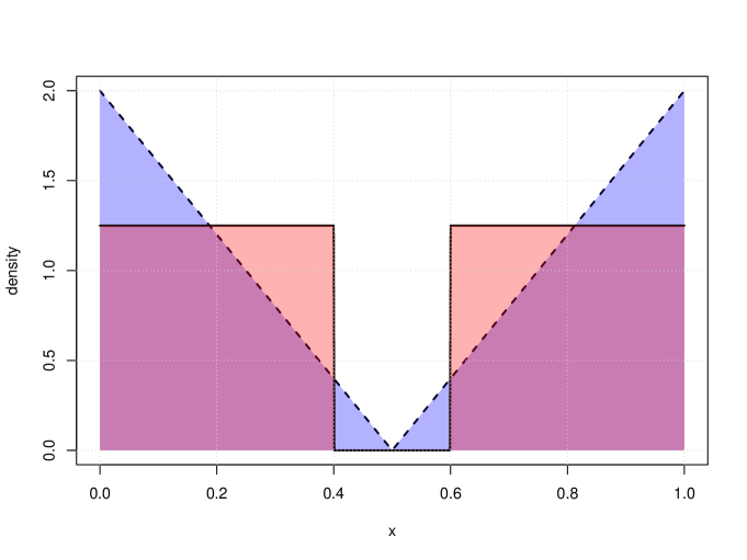
Towards the task of demonstrating empirical evidence of the rates in Theorem 5, we consider the family of beta distributions on the unit interval 𝒳=[0,1]\mathcal{X}=\left[0,1\right] as our base class (i.e., (7)) to estimate a pair of target densities

f1(x)=12χ[0,2/5](x)+12χ[3/5,1](x),f_{1}\left(x\right)=\frac{1}{2}\chi_{\left[0,2/5\right]}\left(x\right)+\frac{1}{2}\chi_{\left[3/5,1\right]}\left(x\right),

and

f2(x)=χ[0,1](x){24xif x1/2,2+4xif x>1/2,f_{2}\left(x\right)=\chi_{\left[0,1\right]}\left(x\right)\begin{cases}2-4x&\text{if }x\leq 1/2,\\ -2+4x&\text{if }x>1/2,\end{cases}

where χ𝒜\chi_{\mathcal{A}} is the characteristic function that takes value 11 if x𝒜x\in\mathcal{A} and 0, otherwise. Note that neither f1f_{1} nor f2f_{2} are in 𝒞\mathcal{C}. In particular, f1(x)=0f_{1}\left(x\right)=0 when x(25,35)x\in\left(\frac{2}{5},\frac{3}{5}\right), and f2(x)=0f_{2}(x)=0 when x=1/2x=1/2, and hence neither densities are bounded away from 0, on 𝒳\mathcal{X}. Thus, the theory of Rakhlin et al. (2005) cannot be applied to provide bounds for the expected KL divergence between MLEs of beta mixtures and the pair of targets. We visualize f1f_{1} and f2f_{2} in Figure 1.

Refer to caption
Figure 1: Simulation target densities f1f_{1} (solid line) and f2f_{2} (dashed line).

To observe the rate of decrease of the hh-lifted KL divergence between the targets and respective sequences of hh-MLLEs, we conduct two experiments E1 and E2. In E1, our target density is set to f1f_{1} and h1=β(;1/2,1/2)h_{1}=\beta\left(\cdot;1/2,1/2\right). For each n{210,,215}n\in\left\{2^{10},\dots,2^{15}\right\} and k{2,,8}k\in\left\{2,\dots,8\right\}, we independently simulate 𝐗n\mathbf{X}_{n} and 𝐘n\mathbf{Y}_{n} with each XiX_{i} and YiY_{i} (i[n]i\in\left[n\right]), i.i.d., from the distributions characterized by f1f_{1} and h1h_{1}, respectively. In E2, we target f2f_{2} with hh-MLLEs over the same ranges of kk and nn, but with h2=β(;1,1)h_{2}=\beta\left(\cdot;1,1\right)–the density of the uniform distribution. For each kk and nn, we simulate 𝐗n\mathbf{X}_{n} and 𝐘n\mathbf{Y}_{n}, respectively, from distributions characterized by f2f_{2} and h2h_{2}.

In both experiments, we simulate r=50r=50 replicates of each (k,n)\left(k,n\right)-scenario and compute the corresponding hh-MLLEs, (fk,n,l)l[r]\left(f_{k,n,l}\right)_{l\in[r]}, using the previously described MM algorithm. For each l[r]l\in\left[r\right], we compute the corresponding negative log hh-lifted likelihood between the target ff and fk,n,lf_{k,n,l}:

Kk,n,l=𝒳(f+h)log(fk,n,l+h)dμK_{k,n,l}=-\int_{\mathcal{X}}\left(f+h\right)\log\left(f_{k,n,l}+h\right)\mathrm{d}\mu

to assess the rates, and note that

KLh(f||fk,n,l)=𝒳(f+h)log(f+h)dμ+Kk,n,l,\mathrm{KL}_{h}\left(f\,||\,f_{k,n,l}\right)=\int_{\mathcal{X}}\left(f+h\right)\log\left(f+h\right)\mathrm{d}\mu+K_{k,n,l},

where the prior term is a constant with respect to kk and nn.

To analyze the sample of 7×6×50=21007\times 6\times 50=2100 observations of relationship between the values (Kk,n,l)l[r]\left(K_{k,n,l}\right)_{l\in[r]} and the corresponding values of kk and nn, we use non-linear least squares (Amemiya, 1985, Sec. 4.3) to fit the regression relationship

𝐄[Kk,n,l]=a0+a1(k+2)b1+a2nb2.{\operatorname*{{\mathrm{\mathbf{E}}}}}\left[K_{k,n,l}\right]=a_{0}+\frac{a_{1}}{\left(k+2\right)^{b_{1}}}+\frac{a_{2}}{n^{b_{2}}}. (10)

We obtain 95%95\% asymptotic confidence intervals for the estimates of the regression parameters a0a_{0}, a1a_{1}, a2a_{2}, b1b_{1}, b2b_{2}\in\mathbb{R}, under the assumption of potential mis-specification of (10), by using the sandwich estimator for the asymptotic covariance matrix (cf. White 1982).

4.3 Results

We report the estimates along with 95%95\% asymptotic confidence intervals for the parameters of (10) for E1 and E2 in Table 1. Plots of the average negative log hh-lifted likelihood values by sample sizes nn and numbers of components kk are provided in Figure 2.

Table 1: Estimates of parameters for fitted relationships (with 95%95\% confidence intervals) between negative log hh-lifted likelihood values, sample size and number of mixture components for experiments E1 and E2.
E1 a0a_{0} a1a_{1} a2a_{2} b1b_{1} b2b_{2}
Est. 1.68-1.68 0.730.73 6.806.80 1.871.87 0.990.99
95% CI (1.68,1.67)\left(-1.68,-1.67\right) (0.68,0.78)\left(0.68,0.78\right) (1.24,12.36)\left(1.24,12.36\right) (1.81,1.93)\left(1.81,1.93\right) (0.87,1.11)\left(0.87,1.11\right)
E2 a0a_{0} a1a_{1} a2a_{2} b1b_{1} b2b_{2}
Est. 1.47-1.47 1.491.49 6.756.75 4.364.36 1.071.07
95% CI (1.48,1.47)\left(-1.48,-1.47\right) (0.58,2.41)\left(0.58,2.41\right) (2.17,11.32)\left(2.17,11.32\right) (3.91,4.81)\left(3.91,4.81\right) (0.97,1.16)\left(0.97,1.16\right)
Refer to caption
Figure 2: Average negative log hh-lifted likelihood values by sample sizes nn and numbers of components kk for experiments E1 and E2.

From Table 1, we observe that 𝐄[Kk,n,l]\operatorname*{{\mathrm{\mathbf{E}}}}\left[K_{k,n,l}\right] decreases with both nn and kk in both simulations, and that the rates at which the averages decrease are faster than anticipated by Theorem 5, with respect to both nn and kk. We can visually confirm the decreases in the estimate of 𝐄[Kk,n,l]\operatorname*{{\mathrm{\mathbf{E}}}}\left[K_{k,n,l}\right] via Figure 2. In both E1 and E2, the rate of decrease over the assessed range of nn is approximately proportional to 1/n1/n, as opposed to the anticipated rate of 1/n1/\sqrt{n}, whereas the rate of decrease in kk is far larger, at approximately 1/k1.871/k^{1.87} for E1 and 1/k4.361/k^{4.36} for E2.

These observations provide empirical evidence towards the fact that the rate of decrease of 𝐄[Kk,n,l]\operatorname*{{\mathrm{\mathbf{E}}}}\left[K_{k,n,l}\right] is at least 1/k1/k and 1/n1/\sqrt{n}, respectively, for kk and nn, at least over the simulation scenarios. These fast rates of fit over small values of nn and kk may be indicative of a diminishing returns of fit phenomenon, as discussed in Cadez & Smyth (2000) or the so-called elbow phenomenon (see, e.g., Ritter 2014, Sec. 4.2), whereupon the rate of decrease in average loss for small values of kk is fast and becomes slower as kk increases, converging to some asymptotic rate. This is also the reason why we do not include the outcomes when k=1k=1, as the drop in 𝐄[Kk,n,l]\operatorname*{{\mathrm{\mathbf{E}}}}\left[K_{k,n,l}\right] between k=1k=1 and k=2k=2 is so dramatic that it makes our simulated data ill-fitted by any model of form (10). As such, we do not view Theorem 5 as being pessimistic in light of these phenomena, as it applies uniformly over all values of kk and nn.

5 Conclusion

The estimation of probability densities using finite mixtures from some base class 𝒫\mathcal{P} appears often in machine learning and statistical inference as a natural method for modelling underlying data generating processes. In this work, we pursue novel generalization bounds for such mixture estimators. To this end, we introduce the family of hh-lifted KL divergences for densities on compact supports, within the family of Bregman divergences, which correspond to risk functions that can be bounded, even when densities in the class 𝒫\mathcal{P} are not bounded away from zero, unlike the standard KL divergence.

Unlike the least-squares loss, the corresponding maximum hh-likelihood estimation problem can be computed via an MM algorithm, mirroring the availability of EM algorithms for the maximum likelihood problem corresponding to the KL divergence. Along with our derivations of generalization bounds that achieve the same rates as the best-known bounds for the KL divergence and least square loss, we also provide numerical evidence towards the correctness of these bounds in the case when 𝒫\mathcal{P} corresponds to beta densities.

Aside from beta distributions, mixture densities on compact supports that can be analysed under our framework appear frequently in the literature. For supports on compact Euclidean subset, examples include mixtures of Dirichlet distributions (Fan et al., 2012) and bivariate binomial distributions (Papageorgiou & David, 1994). Alternatively, one can consider distributions on compact Euclidean manifolds, such as mixtures of Kent (Peel et al., 2001) distributions and von Mises–Fisher distributions (Banerjee et al., 2005, Ng & Kwong, 2022). We defer investigating the practical performance of the maximum hh-lifted likelihood estimators and accompanying theory for such models to future work.

Acknowledgments

We express sincere gratitude to the Reviewers and Action Editor for their valuable feedback, which has helped to improve the quality of this paper. Hien Duy Nguyen and TrungTin Nguyen acknowledge funding from the Australian Research Council grant DP230100905.

References

  • Amari (2016) Shun-ichi Amari. Information Geometry and Its Applications, volume 194. Springer, New York, 2016.
  • Amemiya (1985) Takeshi Amemiya. Advanced econometrics. Harvard University Press, 1985.
  • Banerjee et al. (2005) Arindam Banerjee, Inderjit S Dhillon, Joydeep Ghosh, Suvrit Sra, and Greg Ridgeway. Clustering on the unit hypersphere using von Mises-Fisher distributions. Journal of Machine Learning Research, 6(9), 2005.
  • Bartlett & Mendelson (2002) Peter L Bartlett and Shahar Mendelson. Rademacher and gaussian complexities: Risk bounds and structural results. Journal of Machine Learning Research, 3(Nov):463–482, 2002.
  • Basu et al. (1998) Ayanendranath Basu, Ian R Harris, Nils L Hjort, and MC Jones. Robust and efficient estimation by minimising a density power divergence. Biometrika, 85(3):549–559, 1998.
  • Basu et al. (2011) Ayanendranath Basu, Hiroyuki Shioya, and Chanseok Park. Statistical Inference: The Minimum Distance Approach. CRC press, Boca Raton, 2011.
  • Cadez & Smyth (2000) Igor Cadez and Padhraic Smyth. Model complexity, goodness of fit and diminishing returns. Advances in Neural Information Processing Systems, 13, 2000.
  • Csiszár (1995) Imre Csiszár. Generalized projections for non-negative functions. In Proceedings of 1995 IEEE International Symposium on Information Theory, pp.  6. IEEE, 1995.
  • Dalalyan & Sebbar (2018) Arnak S Dalalyan and Mehdi Sebbar. Optimal kullback–leibler aggregation in mixture density estimation by maximum likelihood. Mathematical Statistics and Learning, 1(1):1–35, 2018.
  • DeVore & Temlyakov (2016) Ronald A DeVore and Vladimir N Temlyakov. Convex optimization on banach spaces. Foundations of Computational Mathematics, 16(2):369–394, 2016.
  • Devroye & Györfi (1985) Luc Devroye and László Györfi. Nonparametric Density Estimation: The L1 View. Wiley Interscience Series in Discrete Mathematics. Wiley, 1985.
  • Devroye & Lugosi (2001) Luc Devroye and Gabor Lugosi. Combinatorial Methods in Density Estimation. Springer Science & Business Media, 2001.
  • Fan et al. (2012) Wentao Fan, Nizar Bouguila, and Djemel Ziou. Variational learning for finite dirichlet mixture models and applications. IEEE transactions on neural networks and learning systems, 23:762–774, 2012.
  • Ferrari & Yang (2010) Davide Ferrari and Yuhong Yang. Maximum lq-likelihood method. Annals of Statistics, 38:573–583, 2010.
  • Frigyik et al. (2008) Béla A Frigyik, Santosh Srivastava, and Maya R Gupta. Functional bregman divergence and bayesian estimation of distributions. IEEE Transactions on Information Theory, 54(11):5130–5139, 2008.
  • Fujisawa & Eguchi (2006) Hironori Fujisawa and Shinto Eguchi. Robust estimation in the normal mixture model. Journal of Statistical Planning and Inference, 136(11):3989–4011, 2006.
  • Ghosal (2001) Subhashis Ghosal. Convergence rates for density estimation with Bernstein polynomials. The Annals of Statistics, 29(5):1264 – 1280, 2001. Publisher: Institute of Mathematical Statistics.
  • Gil et al. (2013) Manuel Gil, Fady Alajaji, and Tamas Linder. Rényi divergence measures for commonly used univariate continuous distributions. Information Sciences, 249:124–131, 2013.
  • Giraud (2021) Christophe Giraud. Introduction to high-dimensional statistics. CRC Press, 2021.
  • Haagerup (1981) Uffe Haagerup. The best constants in the Khintchine inequality. Studia Mathematica, 70(3):231–283, 1981.
  • Hunter & Lange (2004) David R Hunter and Kenneth Lange. A tutorial on mm algorithms. The American Statistician, 58(1):30–37, 2004.
  • Klemelä (2007) Jussi S Klemelä. Density estimation with stagewise optimization of the empirical risk. Machine Learning, 67:169–195, 2007.
  • Klemelä (2009) Jussi S Klemelä. Smoothing of multivariate data: density estimation and visualization. John Wiley & Sons, New York, 2009.
  • Kobayashi & Watanabe (2021) Masahiro Kobayashi and Kazuho Watanabe. Generalized Dirichlet-process-means for f-separable distortion measures. Neurocomputing, 458:667–689, 2021.
  • Kobayashi & Watanabe (2024) Masahiro Kobayashi and Kazuho Watanabe. Unbiased Estimating Equation and Latent Bias under f-Separable Bregman Distortion Measures. IEEE Transactions on Information Theory, 2024.
  • Koltchinskii (2011) Vladimir Koltchinskii. Oracle Inequalities in Empirical Risk Minimization and Sparse Recovery Problems: École D’Été de Probabilités de Saint-Flour XXXVIII-2008. Lecture Notes in Mathematics. Springer, 2011.
  • Koltchinskii & Panchenko (2004) Vladimir Koltchinskii and Dmitry Panchenko. Rademacher processes and bounding the risk of function learning. arXiv: Probability, pp.  443–457, 2004.
  • Kosorok (2007) Michael R. Kosorok. Introduction to Empirical Processes and Semiparametric Inference. Springer Series in Statistics. Springer New York, 2007.
  • Lange (2013) Kenneth Lange. Optimization, volume 95. Springer Science & Business Media, New York, 2013.
  • Lange (2016) Kenneth Lange. MM optimization algorithms. SIAM, Philadelphia, 2016.
  • Li & Barron (1999) Jonathan Li and Andrew Barron. Mixture Density Estimation. In S. Solla, T. Leen, and K. Müller (eds.), Advances in Neural Information Processing Systems, volume 12. MIT Press, 1999.
  • Massart (2007) Pascal Massart. Concentration inequalities and model selection: Ecole d’Eté de Probabilités de Saint-Flour XXXIII-2003. Springer, 2007.
  • Maugis & Michel (2011) Cathy Maugis and Bertrand Michel. A non asymptotic penalized criterion for gaussian mixture model selection. ESAIM: Probability and Statistics, 15:41–68, 2011.
  • Maugis-Rabusseau & Michel (2013) Cathy Maugis-Rabusseau and Bertrand Michel. Adaptive density estimation for clustering with gaussian mixtures. ESAIM: Probability and Statistics, 17:698–724, 2013.
  • McDiarmid (1989) Colin McDiarmid. On the method of bounded differences. In J.Editor Siemons (ed.), Surveys in Combinatorics, 1989: Invited Papers at the Twelfth British Combinatorial Conference, London Mathematical Society Lecture Note Series, pp.  148–188. Cambridge University Press, 1989.
  • McDiarmid (1998) Colin McDiarmid. Concentration. In Michel Habib, Colin McDiarmid, Jorge Ramirez-Alfonsin, and Bruce Reed (eds.), Probabilistic Methods for Algorithmic Discrete Mathematics, pp.  195–248. Springer Berlin Heidelberg, Berlin, Heidelberg, 1998.
  • McLachlan & Peel (2004) Geoffrey J McLachlan and David Peel. Finite Mixture Models. John Wiley & Sons, 2004.
  • Meir & Zeevi (1997) Ronny Meir and Assaf Zeevi. Density estimation through convex combinations of densities: Approximation and estimation bounds. Neural Networks, 10:99–109, 02 1997.
  • Naito & Eguchi (2013) Kanta Naito and Shinto Eguchi. Density estimation with minimization of U-divergence. Machine Learning, 90(1):29–57, January 2013.
  • Ng & Kwong (2022) Tin Lok James Ng and Kwok-Kun Kwong. Universal approximation on the hypersphere. Communications in Statistics-Theory and Methods, 51:8694–8704, 2022.
  • Nguyen (2017) Hien D Nguyen. An introduction to majorization-minimization algorithms for machine learning and statistical estimation. Wiley Interdisciplinary Reviews: Data Mining and Knowledge Discovery, 7(2):e1198, 2017.
  • Nguyen et al. (2021) Hien D Nguyen, TrungTin Nguyen, Faicel Chamroukhi, and Geoffrey J McLachlan. Approximations of conditional probability density functions in Lebesgue spaces via mixture of experts models. Journal of Statistical Distributions and Applications, 8(1):13, August 2021.
  • Nguyen et al. (2022a) Hien D Nguyen, Florence Forbes, Gersende Fort, and Olivier Cappé. An online minorization-maximization algorithm. In Proceedings of the 17th Conference of the International Federation of Classification Societies, 2022a.
  • Nguyen et al. (2020) TrungTin Nguyen, Hien D Nguyen, Faicel Chamroukhi, and Geoffrey J McLachlan. Approximation by finite mixtures of continuous density functions that vanish at infinity. Cogent Mathematics & Statistics, 7:1750861, 2020.
  • Nguyen et al. (2022b) TrungTin Nguyen, Faicel Chamroukhi, Hien D Nguyen, and Geoffrey J McLachlan. Approximation of probability density functions via location-scale finite mixtures in Lebesgue spaces. Communications in Statistics - Theory and Methods, pp.  1–12, 2022b.
  • Nguyen et al. (2022c) TrungTin Nguyen, Hien D Nguyen, Faicel Chamroukhi, and Florence Forbes. A non-asymptotic approach for model selection via penalization in high-dimensional mixture of experts models. Electronic Journal of Statistics, 16(2):4742–4822, 2022c.
  • Papageorgiou & David (1994) Haris Papageorgiou and Katerina M David. On countable mixtures of bivariate binomial distributions. Biometrical journal, 36(5):581–601, 1994.
  • Pardo (2006) Leandro Pardo. Statistical Inference Based on Divergence Measures. CRC Press, Boca Raton, 2006.
  • Peel et al. (2001) David Peel, William J Whiten, and Geoffrey J McLachlan. Fitting mixtures of kent distributions to aid in joint set identification. Journal of the American Statistical Association, 96:56–63, 2001.
  • Petrone (1999) Sonia Petrone. Random Bernstein Polynomials. Scandinavian Journal of Statistics, 26(3):373–393, 1999.
  • Petrone & Wasserman (2002) Sonia Petrone and Larry Wasserman. Consistency of Bernstein Polynomial Posteriors. Journal of the Royal Statistical Society Series B: Statistical Methodology, 64(1):79–100, March 2002.
  • Qin & Priebe (2013) Yichen Qin and Carey E Priebe. Maximum LqL_{q}-likelihood estimation via the expectation-maximization algorithm: a robust estimation of mixture models. Journal of the American Statistical Association, 108(503):914–928, 2013.
  • Rakhlin et al. (2005) Alexander Rakhlin, Dmitry Panchenko, and Sayan Mukherjee. Risk bounds for mixture density estimation. ESAIM: PS, 9:220–229, 2005.
  • Razaviyayn et al. (2013) Meisam Razaviyayn, Mingyi Hong, and Zhi-Quan Luo. A Unified Convergence Analysis of Block Successive Minimization Methods for Nonsmooth Optimization. SIAM Journal on Optimization, 23(2):1126–1153, 2013.
  • Ritter (2014) Gunter Ritter. Robust cluster analysis and variable selection. CRC Press, Boca Raton, 2014.
  • Rockafellar (1997) Ralph Tyrrell Rockafellar. Convex analysis, volume 11. Princeton University Press, Princeton, 1997.
  • Shalev-Shwartz & Ben-David (2014) Shai Shalev-Shwartz and Shai Ben-David. Understanding Machine Learning: from Theory to Algorithms. Cambridge University Press, Cambridge, 2014.
  • Shapiro et al. (2021) Alexander Shapiro, Darinka Dentcheva, and Andrzej Ruszczynski. Lectures on Stochastic Programming: Modeling and Theory, Third Edition. Society for Industrial and Applied Mathematics, Philadelphia, PA, July 2021.
  • Stummer & Vajda (2012) Wolfgang Stummer and Igor Vajda. On bregman distances and divergences of probability measures. IEEE Transactions on Information Theory, 58(3):1277–1288, 2012.
  • Sundberg (2019) Rolf Sundberg. Statistical Modelling by Exponential Families. Cambridge University Press, Cambridge, 2019.
  • Temlyakov (2016) Vladimir N Temlyakov. Convergence and rate of convergence of some greedy algorithms in convex optimization. Proceedings of the Steklov Institute of Mathematics, 293:325–337, 2016.
  • van de Geer (2016) Sara van de Geer. Estimation and Testing Under Sparsity: École d’Été de Probabilités de Saint-Flour XLV – 2015. Springer, 2016.
  • van der Vaart & Wellner (1996) Aad W van der Vaart and Jon A Wellner. Weak Convergence and Empirical Processes: With Applications to Statistics. Springer, 1996.
  • Verbeek et al. (2003) Jakob J Verbeek, Nikos Vlassis, and Ben Kröse. Efficient greedy learning of Gaussian mixture models. Neural computation, 15(2):469–485, 2003.
  • Vlassis & Likas (2002) Nikos Vlassis and Aristidis Likas. A greedy EM algorithm for gaussian mixture learning. Neural Processing Letters, 15:77–87, 2002.
  • White (1982) Halbert White. Maximum likelihood estimation of misspecified models. Econometrica, 50(1):1–25, 1982.
  • Wu & Lange (2010) Tong Tong Wu and Kenneth Lange. The MM alternative to EM. Statistical Science, 25(4):492–505, 2010.
  • Zhang (2003) Tong Zhang. Sequential greedy approximation for certain convex optimization problems. IEEE Transactions on Information Theory, 49(3):682–691, 2003.

Appendix A Proofs of main results

The following section is devoted to establishing some technical definitions and instrumental results which are used to prove Theorem 5 and Corollary 6, and also includes the proofs of these results themselves.

A.1 Preliminaries

Recall that we are interested in bounds of the form (2). Note that 𝒫\mathcal{P} is a subset of the linear space

𝒱=cl(k{j=1kϖjφ(;θj)φ(;θj)𝒫,ϖj,j[k]}),\mathcal{V}=\mathrm{cl}\left(\bigcup_{k\in\mathbb{N}}\left\{\sum_{j=1}^{k}\varpi_{j}\varphi\left(\cdot;\theta_{j}\right)\mid\varphi\left(\cdot;\theta_{j}\right)\in\mathcal{P},\varpi_{j}\in\mathbb{R},j\in\left[k\right]\right\}\right),

and hence we can apply the following result, paraphrased from Zhang (2003, Thm. II.1).

Lemma 8.

Let κ\kappa be a differentiable and convex function on 𝒱\mathcal{V}, and let (f¯k)k\left(\bar{f}_{k}\right)_{k\in\mathbb{N}} be a sequence of functions obtained by Algorithm 1. If

supp,q𝒞,π(0,1)d2dπ2κ((1π)p+πq)𝔐<,\sup_{p,q\in\mathcal{C},\pi\in\left(0,1\right)}\frac{\mathrm{d}^{2}}{\mathrm{d}\pi^{2}}\kappa\left(\left(1-\pi\right)p+\pi q\right)\leq\mathfrak{M}<\infty,

then, for each kk\in\mathbb{N},

κ(f¯k)infp𝒞κ(p)2𝔐k+2.\kappa\left(\bar{f}_{k}\right)-\inf_{p\in\mathcal{C}}\kappa\left(p\right)\leq\frac{2\mathfrak{M}}{k+2}.
Algorithm 1 Algorithm for computing a greedy approximation sequence.
1:f¯0𝒫\bar{f}_{0}\in\mathcal{P}
2:for kk\in\mathbb{N} do
3:     Compute (π¯k,θ¯k)=argmin(π,θ)[0,1]×Θκ((1π)f¯k1+πφ(;θ))\left(\bar{\pi}_{k},\bar{\theta}_{k}\right)=\operatorname*{arg\,min\,}\limits_{\left(\pi,\theta\right)\in[0,1]\times\Theta}\kappa\left(\left(1-\pi\right)\bar{f}_{k-1}+\pi\varphi\left(\cdot;\theta\right)\right)
4:     Define f¯k=(1π¯k)f¯k1+π¯kφ(;θ¯k)\bar{f}_{k}=\left(1-\bar{\pi}_{k}\right)\bar{f}_{k-1}+\bar{\pi}_{k}\varphi\left(\cdot;\bar{\theta}_{k}\right)
5:end for

We are interested in two choices for κ\kappa:

κ(p)=KLh(f||p)\kappa\left(p\right)=\mathrm{KL}_{h}\left(f\,||\,p\right) (11)

and its sample counterpart,

κn(p)=1ni=1nlogf(Xi)+h(Xi)p(Xi)+h(Xi)+1ni=1nlogf(Yi)+h(Yi)p(Yi)+h(Yi),\kappa_{n}\left(p\right)=\frac{1}{n}\sum_{i=1}^{n}\log\frac{f\left(X_{i}\right)+h\left(X_{i}\right)}{p\left(X_{i}\right)+h\left(X_{i}\right)}+\frac{1}{n}\sum_{i=1}^{n}\log\frac{f\left(Y_{i}\right)+h\left(Y_{i}\right)}{p\left(Y_{i}\right)+h\left(Y_{i}\right)}, (12)

where (Xi)i[n](X_{i})_{i\in[n]} and (Yi)i[n](Y_{i})_{i\in[n]} are realisations of XX and YY, respectively. We obtain the following important results.

Proposition 9.

Let ϰ\varkappa denote either κ\kappa, the KLh\mathrm{KL}_{h} divergence (11), or κn\kappa_{n}, the sample KLh\mathrm{KL}_{h} divergence (12), and assume that hah\geq a and φ(;θ)c\varphi\left(\cdot;\theta\right)\leq c, for each θΘ\theta\in\Theta. Then,

ϰ(f¯k)infp𝒞ϰ(p)4a2c2k+2,\varkappa\left(\bar{f}_{k}\right)-\inf_{p\in\mathcal{C}}\varkappa\left(p\right)\leq\frac{4a^{-2}c^{2}}{k+2},

for each kk\in\mathbb{N}, where (f¯k)k\left(\bar{f}_{k}\right)_{k\in\mathbb{N}} is obtained as per Algorithm 1.

Proof.

See Appendix C.4. ∎

Notice that sequences (f¯k)k\left(\bar{f}_{k}\right)_{k\in\mathbb{N}} obtained via Algorithm 1 are greedy approximation sequences, and that f¯k𝒞k\bar{f}_{k}\in\mathcal{C}_{k}, for each kk\in\mathbb{N}. Let (fk)k\left(f_{k}\right)_{k\in\mathbb{N}} be the sequence of minimizers defined by

fk=argminψk𝒮k×ΘkKLh(f||fk(;ψk)),f_{k}=\underset{\psi_{k}\in\mathcal{S}_{k}\times\Theta^{k}}{\operatorname*{arg\,min\,}}\mathrm{KL}_{h}\left(f\,||\,f_{k}\left(\cdot;\psi_{k}\right)\right), (13)

and let (fk,n)k\left(f_{k,n}\right)_{k\in\mathbb{N}} be the sequence of hh-MLLEs, as per (5). Then, by definition, we have the fact that κ(fk)κ(f¯k)\kappa\left(f_{k}\right)\leq\kappa\left(\bar{f}_{k}\right) and κ(fk,n)κ(f¯k)\kappa\left(f_{k,n}\right)\leq\kappa\left(\bar{f}_{k}\right), for κ\kappa set as (11) or (12), respectively. Thus, we have the following result.

Proposition 10.

For the KLh\mathrm{KL}_{h} divergence (11), under the assumption that hah\geq a and φ(;θ)c\varphi\left(\cdot;\theta\right)\leq c, for each θΘ\theta\in\Theta, we have

κ(fk)infp𝒞κ(p)4a2c2k+2\kappa\left(f_{k}\right)-\inf_{p\in\mathcal{C}}\kappa\left(p\right)\leq\frac{4a^{-2}c^{2}}{k+2} (14)

for each kk\in\mathbb{N}, where (fk)k\left(f_{k}\right)_{k\in\mathbb{N}} is the sequence of minimizers defined via (13). Furthermore, for the sample KLh\mathrm{KL}_{h} divergence (12), under the same assumptions as above, we have

κn(fk,n)infp𝒞κn(p)4a2c2k+2,\kappa_{n}\left(f_{k,n}\right)-\inf_{p\in\mathcal{C}}\kappa_{n}\left(p\right)\leq\frac{4a^{-2}c^{2}}{k+2}, (15)

for each kk\in\mathbb{N}, where (fk,n)k\left(f_{k,n}\right)_{k\in\mathbb{N}} are hh-MLLEs defined via (5).

As is common in many statistical learning/uniform convergence results (e.g., Bartlett & Mendelson, 2002, Koltchinskii & Panchenko, 2004), we employ the use of Rademacher processes and associated bounds. Let (εi)i[n](\varepsilon_{i})_{i\in[n]} be i.i.d. Rademacher random variables, that is 𝐏(εi=1)=𝐏(εi=1)=1/2\mathrm{\mathbf{P}}(\varepsilon_{i}=-1)=\mathrm{\mathbf{P}}(\varepsilon_{i}=1)=\nicefrac{{1}}{{2}}, that are independent of (Xi)i[n](X_{i})_{i\in[n]}. The Rademacher process, indexed by a class of real measurable functions 𝒮\mathcal{S}, is defined as the quantity

Rn(s)=1ni=1ns(Xi)εi,R_{n}(s)=\frac{1}{n}\sum_{i=1}^{n}s(X_{i})\varepsilon_{i},

for s𝒮s\in\mathcal{S}. The Rademacher complexity of the class 𝒮\mathcal{S} is given by n(𝒮)=𝐄sups𝒮|Rn(s)|\mathcal{R}_{n}(\mathcal{S})=\operatorname*{{\mathrm{\mathbf{E}}}}\sup_{s\in\mathcal{S}}\lvert R_{n}(s)\rvert.

In the subsequent section, we make use of the following result regarding the supremum of convex functions:

Lemma 11 (Rockafellar, 1997, Thm. 32.2).

Let η\eta be a convex function on a linear space 𝒯\mathcal{T}, and let 𝒮𝒯\mathcal{S}\subset\mathcal{T} be an arbitrary subset. Then,

supp𝒮η(p)=suppco(𝒮)η(p).\sup_{p\in\mathcal{S}}\eta\left(p\right)=\sup_{p\in\mathrm{co}\left(\mathcal{S}\right)}\eta\left(p\right).

In particular, we use the fact that since a linear functional of convex combinations achieves its maximum value at vertices, the Rademacher complexity of 𝒮\mathcal{S} is equal to the Rademacher complexity of co(𝒮)\mathrm{co}(\mathcal{S}) (see Lemma 21). We consequently obtain the following result.

Lemma 12.

Let (εi)i[n](\varepsilon_{i})_{i\in[n]} be i.i.d. Rademacher random variables, independent of (Xi)i[n](X_{i})_{i\in[n]} and 𝒫\mathcal{P} be defined as above. The sets 𝒞\mathcal{C} and 𝒫\mathcal{P} will have equal complexity, n(𝒞)=n(𝒫)\mathcal{R}_{n}(\mathcal{C})=\mathcal{R}_{n}(\mathcal{P}), and the supremum of the Rademacher process indexed by 𝒞\mathcal{C} is equal to the supremum on the basis functions of 𝒫\mathcal{P}:

𝐄εsupg𝒞|1ni=1ng(Xi)εi|=𝐄εsupθΘ|1ni=1nφ(Xi;θ)εi|.{\operatorname*{{\mathrm{\mathbf{E}}}}}_{\varepsilon}\sup_{g\in\mathcal{C}}\left\lvert\frac{1}{n}\sum_{i=1}^{n}g(X_{i})\varepsilon_{i}\right\rvert={\operatorname*{{\mathrm{\mathbf{E}}}}}_{\varepsilon}\sup_{\theta\in\Theta}\left\lvert\frac{1}{n}\sum_{i=1}^{n}\varphi(X_{i};\theta)\varepsilon_{i}\right\rvert.
Proof.

Follows immediately from Lemma 11. ∎

A.2 Proofs

We first present a result establishing a uniform concentration bound for the hh-lifted log-likelihood ratios, which is instrumental in the proof of Theorem 5. Our proofs broadly follow the structure of Rakhlin et al. (2005), modified as needed for the use of KLh\mathrm{KL}_{h}.

Assume that 0φ(;θ)<c0\leq\varphi(\cdot;\theta)<{c} for some c>0c\in\operatorname*{\mathbb{R}}_{>0}. For brevity, we adopt the notation: T(g)𝒞=supg𝒞|T(g)|\left\lVert T(g)\right\rVert_{\mathcal{C}}=\sup_{g\in\mathcal{C}}\lvert T(g)\rvert.

Theorem 13.

Let X1,,XnX_{1},\ldots,X_{n} be an i.i.d. sample of size nn drawn from a fixed density ff such that 0f(x)c0\leq f(x)\leq c for all x𝒳x\in\mathcal{X}, and let hh be a positive density with 0<ah(x)b0<a\leq h(x)\leq b for all x𝒳x\in\mathcal{X}. Then, for each t>0t>0, with probability at least 1et1-\mathrm{e}^{-t},

1ni=1nlogg(Xi)+h(Xi)f(Xi)+h(Xi)𝐄flogg+hf+h𝒞w1n𝐄0clog1/2N(𝒫,ε,dn,x)dε+w2n+w3tn,\left\lVert\frac{1}{n}\sum_{i=1}^{n}\log\frac{g(X_{i})+h(X_{i})}{f(X_{i})+h(X_{i})}-{\operatorname*{{\mathrm{\mathbf{E}}}}}_{f}\log\frac{g+h}{f+h}\right\rVert_{\mathcal{C}}\leq\frac{w_{1}}{\sqrt{n}}\operatorname*{{\mathrm{\mathbf{E}}}}\int_{0}^{c}\log^{1/2}N(\mathcal{P},\varepsilon,d_{n,x})\mathrm{d}\varepsilon+\frac{w_{2}}{\sqrt{n}}+w_{3}\sqrt{\frac{t}{n}},

where w1w_{1}, w2w_{2}, and w3w_{3} are constants that each depend on some or all of aa, bb, and cc, and N(𝒫,ε,dn,x)N(\mathcal{P},\varepsilon,d_{n,x}) is the ε\varepsilon-covering number of 𝒫\mathcal{P} with respect to the following empirical L2L_{2} metric

dn,x2(φ1,φ2)=1ni=1n(φ1(Xi)φ2(Xi))2.d_{n,x}^{2}(\varphi_{1},\varphi_{2})=\frac{1}{n}\sum_{i=1}^{n}(\varphi_{1}(X_{i})-\varphi_{2}(X_{i}))^{2}.
Remark 14.

The bound on the term

1ni=1nlogg(Yi)+h(Yi)f(Yi)+h(Yi)𝐄hlogg+hf+h𝒞\left\lVert\frac{1}{n}\sum_{i=1}^{n}\log\frac{g(Y_{i})+h(Y_{i})}{f(Y_{i})+h(Y_{i})}-{\operatorname*{{\mathrm{\mathbf{E}}}}}_{h}\log\frac{g+h}{f+h}\right\rVert_{\mathcal{C}}

is the same as the above, except where the empirical distance dn,xd_{n,x} is replaced by dn,yd_{n,y}, defined in the same way as dn,xd_{n,x} but with YiY_{i} replacing XiX_{i}.

Proof of Theorem 13.

Fix hh and define the following quantities: g~=g+h\tilde{g}=g+h, f~=f+h\tilde{f}=f+h, 𝒞~=𝒞+h\tilde{\mathcal{C}}=\mathcal{C}+h,

mi=logg~(Xi)f~(Xi),mi=logg~(Xi)f~(Xi),Z(x1,,xn)=1ni=1nlogg~(Xi)f~(Xi)𝐄logg~f~𝒞~.m_{i}=\log\frac{\tilde{g}(X_{i})}{\tilde{f}(X_{i})},\quad m_{i}^{\prime}=\log\frac{\tilde{g}(X_{i}^{\prime})}{\tilde{f}(X_{i}^{\prime})},\quad Z(x_{1},\ldots,x_{n})=\left\lVert\frac{1}{n}\sum_{i=1}^{n}\log\frac{\tilde{g}(X_{i})}{\tilde{f}(X_{i})}-\operatorname*{{\mathrm{\mathbf{E}}}}\log\frac{\tilde{g}}{\tilde{f}}\right\rVert_{\tilde{\mathcal{C}}}.

We first apply McDiarmid’s inequality (Lemma 23) to the random variable ZZ. The bound on the martingale difference is given by

|Z(X1,,Xi,,Xn)Z(X1,,Xi,,Xn)|\displaystyle\left\lvert Z(X_{1},\ldots,X_{i},\ldots,X_{n})-Z(X_{1},\ldots,X_{i}^{\prime},\ldots,X_{n})\right\rvert =|𝐄logg~f~1n(m1++mi++mn)𝒞~\displaystyle=\left\lvert\left\lVert\operatorname*{{\mathrm{\mathbf{E}}}}\log\frac{\tilde{g}}{\tilde{f}}-\frac{1}{n}(m_{1}+\!...\!+m_{i}+\!...\!+m_{n})\right\rVert_{\tilde{\mathcal{C}}}\right.
𝐄logg~f~1n(m1++mi++mn)𝒞~|\displaystyle-\left.\left\lVert\operatorname*{{\mathrm{\mathbf{E}}}}\log\frac{\tilde{g}}{\tilde{f}}-\frac{1}{n}(m_{1}+\!...\!+m_{i}^{\prime}+\!...\!+m_{n})\right\rVert_{\tilde{\mathcal{C}}}\right\rvert
1nlogg~(Xi)f~(Xi)logg~(Xi)f~(Xi)𝒞~\displaystyle\leq\frac{1}{n}\left\lVert\log\frac{\tilde{g}(X_{i}^{\prime})}{\tilde{f}(X_{i}^{\prime})}-\log\frac{\tilde{g}(X_{i})}{\tilde{f}(X_{i})}\right\rVert_{\tilde{\mathcal{C}}}
1n(logc+balogac+b)=1n2logc+ba=ci.\displaystyle\leq\frac{1}{n}\left(\log\frac{c+b}{a}-\log\frac{a}{c+b}\right)=\frac{1}{n}2\log\frac{c+b}{a}=c_{i}.

The chain of inequalities holds because of the triangle inequality and the properties of the supremum. By Lemma 23, we have

𝐏(Z𝐄Z>ε)exp{nε2(2logc+ba)2},{\mathrm{\mathbf{P}}}(Z-\operatorname*{{\mathrm{\mathbf{E}}}}Z>\varepsilon)\leq\exp\left\{-\frac{n\varepsilon^{2}}{(\sqrt{2}\log\frac{c+b}{a})^{2}}\right\},

so

𝐏(Zε+𝐄Z)1exp{nε2(2logc+ba)2},{\mathrm{\mathbf{P}}}(Z\leq\varepsilon+\operatorname*{{\mathrm{\mathbf{E}}}}Z)\geq 1-\exp\left\{-\frac{n\varepsilon^{2}}{(\sqrt{2}\log\frac{c+b}{a})^{2}}\right\},

where it follows from t=nε2/(2logc+ba)2t=n\varepsilon^{2}/(\sqrt{2}\log\frac{c+b}{a})^{2} that ε=2log(c+ba)tn\varepsilon=\sqrt{2}\log\left(\frac{c+b}{a}\right)\sqrt{\frac{t}{n}}. Therefore with probability at least 1et1-\mathrm{e}^{-t},

1ni=1nlogg~(Xi)f~(Xi)𝐄flogg~f~𝒞~𝐄1ni=1nlogg~(Xi)f~(Xi)𝐄flogg~f~𝒞~+2log(c+ba)tn.\left\lVert\frac{1}{n}\sum_{i=1}^{n}\log\frac{\tilde{g}(X_{i})}{\tilde{f}(X_{i})}-{\operatorname*{{\mathrm{\mathbf{E}}}}}_{f}\log\frac{\tilde{g}}{\tilde{f}}\right\rVert_{\tilde{\mathcal{C}}}\leq\operatorname*{{\mathrm{\mathbf{E}}}}\left\lVert\frac{1}{n}\sum_{i=1}^{n}\log\frac{\tilde{g}(X_{i})}{\tilde{f}(X_{i})}-{\operatorname*{{\mathrm{\mathbf{E}}}}}_{f}\log\frac{\tilde{g}}{\tilde{f}}\right\rVert_{\tilde{\mathcal{C}}}+\sqrt{2}\log\left(\frac{c+b}{a}\right)\sqrt{\frac{t}{n}}.

Let (εi)i[n](\varepsilon_{i})_{i\in[n]} be i.i.d. Rademacher random variables, independent of (Xi)i[n](X_{i})_{i\in[n]}. By Lemma 24,

𝐄1ni=1nlogg~(Xi)f~(Xi)𝐄flogg~f~𝒞~2𝐄1ni=1nlogg~(Xi)f~(Xi)εi𝒞~.\operatorname*{{\mathrm{\mathbf{E}}}}\left\lVert\frac{1}{n}\sum_{i=1}^{n}\log\frac{\tilde{g}(X_{i})}{\tilde{f}(X_{i})}-{\operatorname*{{\mathrm{\mathbf{E}}}}}_{f}\log\frac{\tilde{g}}{\tilde{f}}\right\rVert_{\tilde{\mathcal{C}}}\leq 2\operatorname*{{\mathrm{\mathbf{E}}}}\left\lVert\frac{1}{n}\sum_{i=1}^{n}\log\frac{\tilde{g}(X_{i})}{\tilde{f}(X_{i})}\varepsilon_{i}\right\rVert_{\tilde{\mathcal{C}}}.

By combining the results above, the following inequality holds with probability at least 1et1-\mathrm{e}^{-t}

1ni=1nlogg~(Xi)f~(Xi)𝐄flogg~f~𝒞~2𝐄1ni=1nlogg~(Xi)f~(Xi)εi𝒞~+2log(c+ba)tn.\left\lVert\frac{1}{n}\sum_{i=1}^{n}\log\frac{\tilde{g}(X_{i})}{\tilde{f}(X_{i})}-{\operatorname*{{\mathrm{\mathbf{E}}}}}_{f}\log\frac{\tilde{g}}{\tilde{f}}\right\rVert_{\tilde{\mathcal{C}}}\leq 2\operatorname*{{\mathrm{\mathbf{E}}}}\left\lVert\frac{1}{n}\sum_{i=1}^{n}\log\frac{\tilde{g}(X_{i})}{\tilde{f}(X_{i})}\varepsilon_{i}\right\rVert_{\tilde{\mathcal{C}}}+\sqrt{2}\log\left(\frac{c+b}{a}\right)\sqrt{\frac{t}{n}}.

Now let pi=g~(Xi)f~(Xi)1p_{i}=\frac{\tilde{g}(X_{i})}{\tilde{f}(X_{i})}-1, such that ac+bpi+1c+ba\frac{a}{c+b}\leq p_{i}+1\leq\frac{c+b}{a} holds for all i[n]i\in[n]. Additionally, let η(p)=log(p+1)\eta(p)=\log(p+1) so that η(0)=0\eta(0)=0 and note that for p[ac+b1,c+ba1]p\in\left[\frac{a}{c+b}-1,\frac{c+b}{a}-1\right], the derivative of η(p)\eta(p) is maximal at p=ac+b1p^{*}=\frac{a}{c+b}-1, and equal to η(p)=(c+b)/a\eta^{{{}^{\prime}}}(p^{*})=(c+b)/a. Therefore, ab+clog(p+1)\frac{a}{b+c}\log(p+1) is 11-Lipschitz. By Lemma 22 applied to η(p)\eta(p),

2𝐄1ni=1nlogg~(Xi)f~(Xi)εi𝒞~\displaystyle 2\operatorname*{{\mathrm{\mathbf{E}}}}\left\lVert\frac{1}{n}\sum_{i=1}^{n}\log\frac{\tilde{g}(X_{i})}{\tilde{f}(X_{i})}\varepsilon_{i}\right\rVert_{\tilde{\mathcal{C}}} =2𝐄1ni=1nη(pi)εi𝒞~4(c+b)a𝐄1ni=1ng~(Xi)f~(Xi)εi1ni=1nεi𝒞~\displaystyle=2\operatorname*{{\mathrm{\mathbf{E}}}}\left\lVert\frac{1}{n}\sum_{i=1}^{n}\eta(p_{i})\varepsilon_{i}\right\rVert_{\tilde{\mathcal{C}}}\leq\frac{4(c+b)}{a}\operatorname*{{\mathrm{\mathbf{E}}}}\left\lVert\frac{1}{n}\sum_{i=1}^{n}\frac{\tilde{g}(X_{i})}{\tilde{f}(X_{i})}\varepsilon_{i}-\frac{1}{n}\sum_{i=1}^{n}\varepsilon_{i}\right\rVert_{\tilde{\mathcal{C}}}
4(c+b)a𝐄1ni=1ng~(Xi)f~(Xi)εi𝒞~+4(c+b)a𝐄ε|1ni=1nεi|\displaystyle\leq\frac{4(c+b)}{a}\operatorname*{{\mathrm{\mathbf{E}}}}\left\lVert\frac{1}{n}\sum_{i=1}^{n}\frac{\tilde{g}(X_{i})}{\tilde{f}(X_{i})}\varepsilon_{i}\right\rVert_{\tilde{\mathcal{C}}}+\frac{4(c+b)}{a}{\operatorname*{{\mathrm{\mathbf{E}}}}}_{\varepsilon}\left\lvert\frac{1}{n}\sum_{i=1}^{n}\varepsilon_{i}\right\rvert
4(c+b)a𝐄1ni=1ng~(Xi)f~(Xi)εi𝒞~+4(c+b)a1n,\displaystyle\leq\frac{4(c+b)}{a}\operatorname*{{\mathrm{\mathbf{E}}}}\left\lVert\frac{1}{n}\sum_{i=1}^{n}\frac{\tilde{g}(X_{i})}{\tilde{f}(X_{i})}\varepsilon_{i}\right\rVert_{\tilde{\mathcal{C}}}+\frac{4(c+b)}{a}\frac{1}{\sqrt{n}},

where the final inequality follows from the following result, proved in Haagerup (1981):

𝐄ε|1ni=1nεi|(𝐄ε{1ni=1nεi}2)1/2=1n.{\operatorname*{{\mathrm{\mathbf{E}}}}}_{\varepsilon}\left\lvert\frac{1}{n}\sum_{i=1}^{n}\varepsilon_{i}\right\rvert\leq\left({\operatorname*{{\mathrm{\mathbf{E}}}}}_{\varepsilon}\left\{\frac{1}{n}\sum_{i=1}^{n}\varepsilon_{i}\right\}^{2}\right)^{1/2}=\frac{1}{\sqrt{n}}.

Now, let ξi(g~i)=ag~(Xi)/f~(Xi)\xi_{i}(\tilde{g}_{i})=a\cdot{\tilde{g}(X_{i})}/{\tilde{f}(X_{i})}, and note that

|ξi(ui)ξi(vi)|=a|f~(Xi)||u(Xi)v(Xi)||u(Xi)v(Xi)|.\lvert\xi_{i}(u_{i})-\xi_{i}(v_{i})\rvert=\frac{a}{\lvert\tilde{f}(X_{i})\rvert}\lvert u(X_{i})-v(X_{i})\rvert\leq\lvert u(X_{i})-v(X_{i})\rvert.

By again applying Lemma 22, we have

4(c+b)a𝐄1ni=1ng~(Xi)f~(Xi)εi𝒞~\displaystyle\frac{4(c+b)}{a}\operatorname*{{\mathrm{\mathbf{E}}}}\left\lVert\frac{1}{n}\sum_{i=1}^{n}\frac{\tilde{g}(X_{i})}{\tilde{f}(X_{i})}\varepsilon_{i}\right\rVert_{\tilde{\mathcal{C}}} 8(c+b)a2𝐄1ni=1ng~(Xi)εi𝒞~\displaystyle\leq\frac{8(c+b)}{a^{2}}\operatorname*{{\mathrm{\mathbf{E}}}}\left\lVert\frac{1}{n}\sum_{i=1}^{n}\tilde{g}(X_{i})\varepsilon_{i}\right\rVert_{\tilde{\mathcal{C}}}
8(c+b)a2𝐄1ni=1ng(Xi)εi𝒞+8(c+b)a2𝐄|1ni=1nh(Xi)εi|\displaystyle\leq\frac{8(c+b)}{a^{2}}\operatorname*{{\mathrm{\mathbf{E}}}}\left\lVert\frac{1}{n}\sum_{i=1}^{n}g(X_{i})\varepsilon_{i}\right\rVert_{\mathcal{C}}+\frac{8(c+b)}{a^{2}}\operatorname*{{\mathrm{\mathbf{E}}}}\left\lvert\frac{1}{n}\sum_{i=1}^{n}h(X_{i})\varepsilon_{i}\right\rvert
8(c+b)a2𝐄1ni=1ng(Xi)εi𝒞+8(c+b)a2bn.\displaystyle\leq\frac{8(c+b)}{a^{2}}\operatorname*{{\mathrm{\mathbf{E}}}}\left\lVert\frac{1}{n}\sum_{i=1}^{n}g(X_{i})\varepsilon_{i}\right\rVert_{\mathcal{C}}+\frac{8(c+b)}{a^{2}}\frac{b}{\sqrt{n}}.

Applying Lemmas 12 and 25, the following inequality holds for some constant K>0K>0:

𝐄εsupg𝒞|1ni=1ng(Xi)εi|=𝐄εsupθΘ|1ni=1nφ(Xi;θ)εi|Kn𝐄0clog1/2N(𝒫,ε,dn,x)dε,{\operatorname*{{\mathrm{\mathbf{E}}}}}_{\varepsilon}\sup_{g\in\mathcal{C}}\left\lvert\frac{1}{n}\sum_{i=1}^{n}g(X_{i})\varepsilon_{i}\right\rvert={\operatorname*{{\mathrm{\mathbf{E}}}}}_{\varepsilon}\sup_{\theta\in\Theta}\left\lvert\frac{1}{n}\sum_{i=1}^{n}\varphi(X_{i};\theta)\varepsilon_{i}\right\rvert\leq\frac{K}{\sqrt{n}}\operatorname*{{\mathrm{\mathbf{E}}}}\int_{0}^{c}\log^{1/2}N(\mathcal{P},\varepsilon,d_{n,x})\mathrm{d}\varepsilon, (16)

and combining the results together, the following inequality holds with probability at least 1et1-\mathrm{e}^{-t}:

1ni=1nlogg~(Xi)f~(Xi)𝐄flogg~f~\displaystyle\left\lVert\frac{1}{n}\sum_{i=1}^{n}\log\frac{\tilde{g}(X_{i})}{\tilde{f}(X_{i})}-{\operatorname*{{\mathrm{\mathbf{E}}}}}_{f}\log\frac{\tilde{g}}{\tilde{f}}\right\rVert 8(c+b)Ka2n𝐄0clog1/2N(𝒫,ε,dn,x)dε+(8b+4a)(c+b)a2n+2log(c+ba)tn\displaystyle\leq\frac{8(c+b)K}{a^{2}\sqrt{n}}\operatorname*{{\mathrm{\mathbf{E}}}}\int_{0}^{c}\log^{1/2}N(\mathcal{P},\varepsilon,d_{n,x})\mathrm{d}\varepsilon+\frac{(8b+4a)(c+b)}{a^{2}\sqrt{n}}+\sqrt{2}\log\left(\frac{c+b}{a}\right)\sqrt{\frac{t}{n}}
=w1n𝐄0clog1/2N(𝒫,ε,dn,x)dε+w2n+w3tn,\displaystyle=\frac{w_{1}}{\sqrt{n}}\operatorname*{{\mathrm{\mathbf{E}}}}\int_{0}^{c}\log^{1/2}N(\mathcal{P},\varepsilon,d_{n,x})\mathrm{d}\varepsilon+\frac{w_{2}}{\sqrt{n}}+w_{3}\sqrt{\frac{t}{n}}, (17)

where w1w_{1}, w2w_{2}, and w3w_{3} are constants that each depend on some or all of aa, bb, and cc. ∎

Remark 15.

From Lemma 25 we have that σn2supfPnf2\sigma^{2}_{n}\coloneqq\sup_{f\in\mathscr{F}}P_{n}f^{2}. To make explicit why 2σn=(supg𝒞Png2)1/2=2c2\sigma_{n}=\left(\sup_{g\in\mathcal{C}}P_{n}g^{2}\right)^{1/2}=2c, let =𝒞\mathscr{F}=\mathcal{C} and observe

σn2=supg𝒞Png2=supg𝒞1ni=1ng(Xi)21ni=1nc2=c2.\sigma^{2}_{n}=\sup_{g\in\mathcal{C}}P_{n}g^{2}=\sup_{g\in\mathcal{C}}\frac{1}{n}\sum_{i=1}^{n}g(X_{i})^{2}\leq\frac{1}{n}\sum_{i=1}^{n}c^{2}=c^{2}.

Since our basis functions φ(,θ)\varphi(\cdot,\theta) are bounded by cc, everything greater than cc will have value 0 and hence the change from 2c2c to cc is inconsequential. However, it can also be motivated by the fact that φ(,θ)\varphi(\cdot,\theta) are positive functions.

As highlighted in Remark 14, the full result of Theorem 13 relies on the empirical L2L_{2} distances dn,xd_{n,x} and dn,yd_{n,y}. In the result of Theorem 5, we make use of the following result to bound dn,xd_{n,x} and dn,yd_{n,y}.

Proposition 16.

By combining Lemmas 18 and 19, the following inequalities holds:

logN(𝒫,ε,)logN[](𝒫,ε,)logN(𝒫,ε/2,),\log N(\mathcal{P},\varepsilon,\operatorname*{\lVert\,\cdot\,\rVert})\leq\log N_{[]}(\mathcal{P},\varepsilon,\operatorname*{\lVert\,\cdot\,\rVert})\leq\log N(\mathcal{P},\varepsilon/2,{\operatorname*{\lVert\,\cdot\,\rVert}}_{\infty}),

where N[](𝒫,ε,)N_{[]}(\mathcal{P},\varepsilon,\operatorname*{\lVert\,\cdot\,\rVert}) is the ε\varepsilon-bracketing number of 𝒫\mathcal{P}. Therefore, we have that

logN(𝒫,ε,dn,x)logN(𝒫,ε/2,), and logN(𝒫,ε,dn,y)logN(𝒫,ε/2,).\log N(\mathcal{P},\varepsilon,d_{n,x})\leq\log N(\mathcal{P},\varepsilon/2,{\operatorname*{\lVert\,\cdot\,\rVert}}_{\infty}),\text{ and }\log N(\mathcal{P},\varepsilon,d_{n,y})\leq\log N(\mathcal{P},\varepsilon/2,{\operatorname*{\lVert\,\cdot\,\rVert}}_{\infty}).

With this result, we can now prove Theorem 5.

Proof (of Theorem 5).

The notation is the same as in the proof of Theorem 13. The values of the constants may change from line to line.

KLh(f||fk,n)KLh(f||fk)=𝐄flogf~f~k,n+𝐄hlogf~f~k,n𝐄flogf~f~k𝐄hlogf~f~k\displaystyle\mathrm{KL}_{h}\left(f\,||\,f_{k,n}\right)-\mathrm{KL}_{h}\left(f\,||\,f_{k}\right)={\operatorname*{{\mathrm{\mathbf{E}}}}}_{f}\log\frac{\tilde{f}}{\tilde{f}_{k,n}}+{\operatorname*{{\mathrm{\mathbf{E}}}}}_{h}\log\frac{\tilde{f}}{\tilde{f}_{k,n}}-{\operatorname*{{\mathrm{\mathbf{E}}}}}_{f}\log\frac{\tilde{f}}{\tilde{f}_{k}}-{\operatorname*{{\mathrm{\mathbf{E}}}}}_{h}\log\frac{\tilde{f}}{\tilde{f}_{k}}
=𝐄flogf~f~k,n1ni=1nlogf~(Xi)f~k,n(Xi)+1ni=1nlogf~(Xi)f~k,n(Xi)+𝐄hlogf~f~k,n1ni=1nlogf~(Yi)f~k,n(Yi)+1ni=1nlogf~(Yi)f~k,n(Yi)\displaystyle\ ={\operatorname*{{\mathrm{\mathbf{E}}}}}_{f}\log\frac{\tilde{f}}{\tilde{f}_{k,n}}-\frac{1}{n}\sum_{i=1}^{n}\log\frac{\tilde{f}(X_{i})}{\tilde{f}_{k,n}(X_{i})}+\frac{1}{n}\sum_{i=1}^{n}\log\frac{\tilde{f}(X_{i})}{\tilde{f}_{k,n}(X_{i})}+{\operatorname*{{\mathrm{\mathbf{E}}}}}_{h}\log\frac{\tilde{f}}{\tilde{f}_{k,n}}-\frac{1}{n}\sum_{i=1}^{n}\log\frac{\tilde{f}(Y_{i})}{\tilde{f}_{k,n}(Y_{i})}+\frac{1}{n}\sum_{i=1}^{n}\log\frac{\tilde{f}(Y_{i})}{\tilde{f}_{k,n}(Y_{i})}
𝐄flogf~f~k+1ni=1nlogf~(Xi)f~k(Xi)1ni=1nlogf~(Xi)f~k(Xi)𝐄hlogf~f~k+1ni=1nlogf~(Yi)f~k(Yi)1ni=1nlogf~(Yi)f~k(Yi)\displaystyle\ \qquad-{\operatorname*{{\mathrm{\mathbf{E}}}}}_{f}\log\frac{\tilde{f}}{\tilde{f}_{k}}+\frac{1}{n}\sum_{i=1}^{n}\log\frac{\tilde{f}(X_{i})}{\tilde{f}_{k}(X_{i})}-\frac{1}{n}\sum_{i=1}^{n}\log\frac{\tilde{f}(X_{i})}{\tilde{f}_{k}(X_{i})}-{\operatorname*{{\mathrm{\mathbf{E}}}}}_{h}\log\frac{\tilde{f}}{\tilde{f}_{k}}+\frac{1}{n}\sum_{i=1}^{n}\log\frac{\tilde{f}(Y_{i})}{\tilde{f}_{k}(Y_{i})}-\frac{1}{n}\sum_{i=1}^{n}\log\frac{\tilde{f}(Y_{i})}{\tilde{f}_{k}(Y_{i})}
=(𝐄flogf~f~k,n1ni=1nlogf~(Xi)f~k,n(Xi))+(𝐄hlogf~f~k,n1ni=1nlogf~(Yi)f~k,n(Yi))\displaystyle\ =\left({\operatorname*{{\mathrm{\mathbf{E}}}}}_{f}\log\frac{\tilde{f}}{\tilde{f}_{k,n}}-\frac{1}{n}\sum_{i=1}^{n}\log\frac{\tilde{f}(X_{i})}{\tilde{f}_{k,n}(X_{i})}\right)+\left({\operatorname*{{\mathrm{\mathbf{E}}}}}_{h}\log\frac{\tilde{f}}{\tilde{f}_{k,n}}-\frac{1}{n}\sum_{i=1}^{n}\log\frac{\tilde{f}(Y_{i})}{\tilde{f}_{k,n}(Y_{i})}\right)
+(1ni=1nlogf~(Xi)f~k(Xi)𝐄flogf~f~k)+(1ni=1nlogf~(Yi)f~k(Yi)𝐄hlogf~f~k)\displaystyle\ \quad+\left(\frac{1}{n}\sum_{i=1}^{n}\log\frac{\tilde{f}(X_{i})}{\tilde{f}_{k}(X_{i})}-{\operatorname*{{\mathrm{\mathbf{E}}}}}_{f}\log\frac{\tilde{f}}{\tilde{f}_{k}}\right)+\left(\frac{1}{n}\sum_{i=1}^{n}\log\frac{\tilde{f}(Y_{i})}{\tilde{f}_{k}(Y_{i})}-{\operatorname*{{\mathrm{\mathbf{E}}}}}_{h}\log\frac{\tilde{f}}{\tilde{f}_{k}}\right)
+(1ni=1nlogf~(Xi)f~k,n(Xi)1ni=1nlogf~(Xi)f~k(Xi))+(1ni=1nlogf~(Yi)f~k,n(Yi)1ni=1nlogf~(Yi)f~k(Yi))\displaystyle\ \quad+\left(\frac{1}{n}\sum_{i=1}^{n}\log\frac{\tilde{f}(X_{i})}{\tilde{f}_{k,n}(X_{i})}-\frac{1}{n}\sum_{i=1}^{n}\log\frac{\tilde{f}(X_{i})}{\tilde{f}_{k}(X_{i})}\right)+\left(\frac{1}{n}\sum_{i=1}^{n}\log\frac{\tilde{f}(Y_{i})}{\tilde{f}_{k,n}(Y_{i})}-\frac{1}{n}\sum_{i=1}^{n}\log\frac{\tilde{f}(Y_{i})}{\tilde{f}_{k}(Y_{i})}\right)
2supg~𝒞~|1ni=1nlogg~(Xi)f~(Xi)𝐄flogg~f~|+2supg~𝒞~|1ni=1nlogg~(Yi)f~(Yi)𝐄hlogg~f~|\displaystyle\ \leq 2\sup_{\tilde{g}\in\tilde{\mathcal{C}}}\left\lvert\frac{1}{n}\sum_{i=1}^{n}\log\frac{\tilde{g}(X_{i})}{\tilde{f}(X_{i})}-{\operatorname*{{\mathrm{\mathbf{E}}}}}_{f}\log\frac{\tilde{g}}{\tilde{f}}\right\rvert+2\sup_{\tilde{g}\in\tilde{\mathcal{C}}}\left\lvert\frac{1}{n}\sum_{i=1}^{n}\log\frac{\tilde{g}(Y_{i})}{\tilde{f}(Y_{i})}-{\operatorname*{{\mathrm{\mathbf{E}}}}}_{h}\log\frac{\tilde{g}}{\tilde{f}}\right\rvert
+(1ni=1nlogf~(Xi)f~k,n(Xi)1ni=1nlogf~(Xi)f~k(Xi))+(1ni=1nlogf~(Yi)f~k,n(Yi)1ni=1nlogf~(Yi)f~k(Yi))\displaystyle\ \quad+\left(\frac{1}{n}\sum_{i=1}^{n}\log\frac{\tilde{f}(X_{i})}{\tilde{f}_{k,n}(X_{i})}-\frac{1}{n}\sum_{i=1}^{n}\log\frac{\tilde{f}(X_{i})}{\tilde{f}_{k}(X_{i})}\right)+\left(\frac{1}{n}\sum_{i=1}^{n}\log\frac{\tilde{f}(Y_{i})}{\tilde{f}_{k,n}(Y_{i})}-\frac{1}{n}\sum_{i=1}^{n}\log\frac{\tilde{f}(Y_{i})}{\tilde{f}_{k}(Y_{i})}\right)
2𝐄{w1xn0clog1/2N(𝒫,ε,dn,x)dε}+w2xn+w3xtn+1ni=1nlogf~k(Xi)f~k,n(Xi)\displaystyle\ \leq 2\operatorname*{{\mathrm{\mathbf{E}}}}\left\{\frac{w^{x}_{1}}{\sqrt{n}}\int_{0}^{c}\log^{1/2}N(\mathcal{P},\varepsilon,d_{n,x})\mathrm{d}\varepsilon\right\}+\frac{w^{x}_{2}}{\sqrt{n}}+w^{x}_{3}\sqrt{\frac{t}{n}}+\frac{1}{n}\sum_{i=1}^{n}\log\frac{\tilde{f}_{k}(X_{i})}{\tilde{f}_{k,n}(X_{i})}
+2𝐄{w1yn0clog1/2N(𝒫,ε,dn,y)dε}+w2yn+w3ytn+1ni=1nlogf~k(Yi)f~k,n(Yi)\displaystyle\ \qquad+2\operatorname*{{\mathrm{\mathbf{E}}}}\left\{\frac{w^{y}_{1}}{\sqrt{n}}\int_{0}^{c}\log^{1/2}N(\mathcal{P},\varepsilon,d_{n,y})\mathrm{d}\varepsilon\right\}+\frac{w^{y}_{2}}{\sqrt{n}}+w^{y}_{3}\sqrt{\frac{t}{n}}+\frac{1}{n}\sum_{i=1}^{n}\log\frac{\tilde{f}_{k}(Y_{i})}{\tilde{f}_{k,n}(Y_{i})}
w1n0clog1/2N(𝒫,ε/2,)dε+w2n+w3tn+1ni=1nlogf~k(Xi)f~k,n(Xi)+1ni=1nlogf~k(Yi)f~k,n(Yi),\displaystyle\ \leq\frac{w_{1}}{\sqrt{n}}\int_{0}^{c}\log^{1/2}N(\mathcal{P},\varepsilon/2,{\operatorname*{\lVert\,\cdot\,\rVert}}_{\infty})\mathrm{d}\varepsilon+\frac{w_{2}}{\sqrt{n}}+w_{3}\sqrt{\frac{t}{n}}+\frac{1}{n}\sum_{i=1}^{n}\log\frac{\tilde{f}_{k}(X_{i})}{\tilde{f}_{k,n}(X_{i})}+\frac{1}{n}\sum_{i=1}^{n}\log\frac{\tilde{f}_{k}(Y_{i})}{\tilde{f}_{k,n}(Y_{i})},

with probability at least 1et1-\mathrm{e}^{-t}, by Theorem 13. Now, we can use (15) from Proposition 10 applied to the target density fkf_{k}, obtaining the following:

KLh(fk||fk,n)\displaystyle\mathrm{KL}_{h}\left(f_{k}\,||\,f_{k,n}\right) =1ni=1nlogf~k(Xi)f~k,n(Xi)+1ni=1nlogf~k(Yi)f~k,n(Yi)4a2c2k+2+infp𝒞KLh(fk||p).\displaystyle=\frac{1}{n}\sum_{i=1}^{n}\log\frac{\tilde{f}_{k}(X_{i})}{\tilde{f}_{k,n}(X_{i})}+\frac{1}{n}\sum_{i=1}^{n}\log\frac{\tilde{f}_{k}(Y_{i})}{\tilde{f}_{k,n}(Y_{i})}\leq\frac{4a^{-2}c^{2}}{k+2}+\inf_{p\in\mathcal{C}}\mathrm{KL}_{h}\left(f_{k}\,||\,p\right).

Since by definition we have that fk𝒞f_{k}\in\mathcal{C}, infp𝒞KLh(fk||p)=0\inf_{p\in\mathcal{C}}\mathrm{KL}_{h}\left(f_{k}\,||\,p\right)=0, and so with probability at least 1et1-\mathrm{e}^{-t} we have:

KLh(f||fk,n)\displaystyle\mathrm{KL}_{h}\left(f\,||\,f_{k,n}\right) KLh(f||fk)w1n0clog1/2N(𝒫,ε/2,)dε+w2n+w3tn+w4k+2.\displaystyle-\mathrm{KL}_{h}\left(f\,||\,f_{k}\right)\leq\frac{w_{1}}{\sqrt{n}}\int_{0}^{c}\log^{1/2}N(\mathcal{P},\varepsilon/2,{\operatorname*{\lVert\,\cdot\,\rVert}}_{\infty})\mathrm{d}\varepsilon+\frac{w_{2}}{\sqrt{n}}+w_{3}\sqrt{\frac{t}{n}}+\frac{w_{4}}{k+2}. (18)

We can write the overall error as the sum of the approximation and estimation errors as follows. The former is bounded by (14), and the latter is bounded as above in (18). Therefore, with probability at least 1et1-\mathrm{e}^{-t},

KLh(f||fk,n)KLh(f||𝒞)\displaystyle\mathrm{KL}_{h}\left(f\,||\,f_{k,n}\right)-\mathrm{KL}_{h}\left(f\,||\,\mathcal{C}\right) =[KLh(f||fk)KLh(f||𝒞)]+[KLh(f||fk,n)KLh(f||fk)]\displaystyle=[\mathrm{KL}_{h}\left(f\,||\,f_{k}\right)-\mathrm{KL}_{h}\left(f\,||\,\mathcal{C}\right)]+[\mathrm{KL}_{h}\left(f\,||\,f_{k,n}\right)-\mathrm{KL}_{h}\left(f\,||\,f_{k}\right)]
w4k+2+w1n0clog1/2N(𝒫,ε/2,)dε+w2n+w3tn.\displaystyle\leq\frac{w_{4}}{k+2}+\frac{w_{1}}{\sqrt{n}}\int_{0}^{c}\log^{1/2}N(\mathcal{P},\varepsilon/2,{\operatorname*{\lVert\,\cdot\,\rVert}}_{\infty})\mathrm{d}\varepsilon+\frac{w_{2}}{\sqrt{n}}+w_{3}\sqrt{\frac{t}{n}}. (19)

As in Rakhlin et al. (2005), we rewrite the above probabilistic statement as a statement in terms of expectations. To this end, let

𝒜w4k+2+w1n0clog1/2N(𝒫,ε/2,)dε+w2n,\mathcal{A}\coloneqq\frac{w_{4}}{k+2}+\frac{w_{1}}{\sqrt{n}}\int_{0}^{c}\log^{1/2}N(\mathcal{P},\varepsilon/2,{\operatorname*{\lVert\,\cdot\,\rVert}}_{\infty})\mathrm{d}\varepsilon+\frac{w_{2}}{\sqrt{n}},

and 𝒵KLh(f||fk,n)KLh(f||𝒞)\mathcal{Z}\coloneqq\mathrm{KL}_{h}\left(f\,||\,f_{k,n}\right)-\mathrm{KL}_{h}\left(f\,||\,\mathcal{C}\right). We have shown 𝐏(𝒵𝒜+w3tn)et{\mathrm{\mathbf{P}}}\left(\mathcal{Z}\geq\mathcal{A}+w_{3}\sqrt{\frac{t}{n}}\right)\leq\mathrm{e}^{-t}. Since 𝒵0\mathcal{Z}\geq 0,

𝐄{𝒵}=0𝒜𝐏(𝒵>s)ds+𝒜𝐏(𝒵>s)ds𝒜+0𝐏(𝒵>𝒜+s)ds.\operatorname*{{\mathrm{\mathbf{E}}}}\{\mathcal{Z}\}=\int^{\mathcal{A}}_{0}{\mathrm{\mathbf{P}}}(\mathcal{Z}>s)\mathrm{d}s+\int^{\infty}_{\mathcal{A}}{\mathrm{\mathbf{P}}}(\mathcal{Z}>s)\mathrm{d}s\leq\mathcal{A}+\int_{0}^{\infty}{\mathrm{\mathbf{P}}}(\mathcal{Z}>\mathcal{A}+s)\mathrm{d}s.

Setting s=w3tns=w_{3}\sqrt{\frac{t}{n}}, we have t=w5ns2t=w_{5}ns^{2} and 𝐄{𝒵}𝒜+0ew5ns2ds𝒜+wn\operatorname*{{\mathrm{\mathbf{E}}}}\{\mathcal{Z}\}\leq\mathcal{A}+\int_{0}^{\infty}e^{-w_{5}ns^{2}}\mathrm{d}s\leq\mathcal{A}+\frac{w}{\sqrt{n}}. Hence,

𝐄{KLh(f||fk,n)}KLh(f||𝒞)c1k+2+c2n0clog1/2N(𝒫,ε/2,)dε+c3n,{\operatorname*{{\mathrm{\mathbf{E}}}}}\left\{\mathrm{KL}_{h}\left(f\,||\,f_{k,n}\right)\right\}-\mathrm{KL}_{h}\left(f\,||\,\mathcal{C}\right)\leq\frac{c_{1}}{k+2}+\frac{c_{2}}{\sqrt{n}}\int_{0}^{c}\log^{1/2}N\left(\mathcal{P},\varepsilon/2,{\operatorname*{\lVert\,\cdot\,\rVert}}_{\infty}\right)\mathrm{d}\varepsilon+\frac{c_{3}}{\sqrt{n}},

where c1c_{1}, c2c_{2}, and c3c_{3} are constants that depend on some or all of aa, bb, and cc. ∎

Remark 17.

The approximation error characterises the suitability of the class 𝒞\mathcal{C}, i.e., how well functions in 𝒞\mathcal{C} are able to estimate a target ff which does not necessarily lie in 𝒞\mathcal{C}. The estimation error characterises the error arising from the estimation of the target ff on the basis of the finite sample of size nn.

Proof of Corollary 6.

Let 𝒳\mathcal{X} and Θ\Theta be compact and assume the Lipshitz condition given in (8). If φ(x;)\varphi(x;\cdot) is continuously differentiable, then

|φ(x;θ)φ(x;τ)|\displaystyle\left|\varphi\left(x;\theta\right)-\varphi\left(x;\tau\right)\right| k=1d|φ(x;)θk(θk)||θkτk|supθΘφ(x;)θ(θ)1θτ1.\displaystyle\leq\sum_{k=1}^{d}\left|\frac{\partial\varphi\left(x;\cdot\right)}{\partial\theta_{k}}\left(\theta_{k}^{*}\right)\right|\left|\theta_{k}-\tau_{k}\right|\leq\sup_{\theta^{*}\in\Theta}\left\|\frac{\partial\varphi\left(x;\cdot\right)}{\partial\theta}\left(\theta^{*}\right)\right\|_{1}\left\|\theta-\tau\right\|_{1}.

Setting

Φ(x)=supθΘφ(x;)θ(θ)1,\varPhi\left(x\right)=\sup_{\theta^{*}\in\Theta}\left\|\frac{\partial\varphi\left(x;\cdot\right)}{\partial\theta}\left(\theta^{*}\right)\right\|_{1},

we have Φ<\lVert\varPhi\rVert_{\infty}<\infty. From Lemma 20, we obtain the fact that

logN[](𝒫,2εΦ,)logN(Θ,ε,),\log N_{[]}\left(\mathcal{P},2\varepsilon\lVert\varPhi\rVert_{\infty},{\operatorname*{\lVert\,\cdot\,\rVert}}_{\infty}\right)\leq\log N\left(\Theta,\varepsilon,{\operatorname*{\lVert\,\cdot\,\rVert}}_{\infty}\right),

which by the change of variable δ=2εΦε=δ/2Φ\delta=2\varepsilon\lVert\varPhi\rVert_{\infty}\implies\varepsilon=\delta/2\lVert\varPhi\rVert_{\infty} implies

logN[](𝒫,ε/2,)logN(Θ,ε4Φ,1).\log N_{[]}\left(\mathcal{P},\varepsilon/2,{\operatorname*{\lVert\,\cdot\,\rVert}}_{\infty}\right)\leq\log N\left(\Theta,\frac{\varepsilon}{4\lVert\varPhi\rVert_{\infty}},{\operatorname*{\lVert\,\cdot\,\rVert}}_{1}\right).

Since Θd\Theta\subset\mathbb{R}^{d}, using the fact that a Euclidean set of radius rr has covering number N(r,ε)(3rε)d,N\left(r,\varepsilon\right)\leq\left(\frac{3r}{\varepsilon}\right)^{d}, we have

logN(Θ,ε4Φ,1)dlog[12Φdiam(Θ)ε].\log N\left(\Theta,\frac{\varepsilon}{4\lVert\varPhi\rVert_{\infty}},{\operatorname*{\lVert\,\cdot\,\rVert}}_{1}\right)\leq d\log\left[\frac{12\lVert\varPhi\rVert_{\infty}\mathrm{diam}\left(\Theta\right)}{\varepsilon}\right].

So

0clogN(Θ,ε4Φ,1)dε0cdlog[12Φdiam(Θ)ε]dε,\int_{0}^{c}\sqrt{\log N\left(\Theta,\frac{\varepsilon}{4\lVert\varPhi\rVert_{\infty}},{\operatorname*{\lVert\,\cdot\,\rVert}}_{1}\right)}\mathrm{d}\varepsilon\leq\int_{0}^{c}\sqrt{d\log\left[\frac{12\lVert\varPhi\rVert_{\infty}\mathrm{diam}\left(\Theta\right)}{\varepsilon}\right]}\mathrm{d}\varepsilon,

and since c<c<\infty, the integral is finite, as required. ∎

Appendix B Discussions and remarks regarding hh-MLLEs

In this section, we share some commentary on the derivation of the hh-lifted KL divergence, its advantages and drawbacks, and some thoughts on the selection of the lifting function hh. We also discuss the suitability of the MM algorithms in contrast to other approaches (e.g., EM algorithms).

B.1 Elementary derivation

From Equation 4, we observe that if XX arises from a measure with density ff, and if we aim to approximate ff with a density gcok(𝒫)g\in\mathrm{co}_{k}(\mathcal{P}) that minimizes the hh-lifted KL divergence KLh\mathrm{KL}_{h} with respect to ff, then we can define an approximator (referred to as the minimum hh-lifted KL approximator) as

fk\displaystyle f_{k} =argmingcok(𝒫)[𝒳{f+h}log{f+h}dμ𝒳{f+h}log{g+h}dμ]\displaystyle=\underset{g\in\mathrm{co}_{k}(\mathcal{P})}{\operatorname*{arg\,min\,}}\left[\int_{\mathcal{X}}\{f+h\}\log\{f+h\}\mathrm{d}\mu-\int_{\mathcal{X}}\{f+h\}\log\{g+h\}\mathrm{d}\mu\right]
=argmingcok(𝒫)𝒳{f+h}log{g+h}dμ=argmaxgcok(𝒫)𝒳{f+h}log{g+h}dμ,\displaystyle=\underset{g\in\mathrm{co}_{k}(\mathcal{P})}{\operatorname*{arg\,min\,}}-\int_{\mathcal{X}}\{f+h\}\log\{g+h\}\mathrm{d}\mu=\underset{g\in\mathrm{co}_{k}(\mathcal{P})}{\operatorname*{arg\,max\,}}\int_{\mathcal{X}}\{f+h\}\log\{g+h\}\mathrm{d}\mu,

noting that 𝒳{f+h}log{f+h}dμ\int_{\mathcal{X}}\{f+h\}\log\{f+h\}\mathrm{d}\mu is a constant that does not depend on the argument gg. Now, observe that

𝒳flog{g+h}dμ=𝐄flog{g+h} and 𝒳flog{g+h}dμ=𝐄flog{g+h},\displaystyle\int_{\mathcal{X}}f\log\{g+h\}\mathrm{d}\mu={\operatorname*{{\mathrm{\mathbf{E}}}}}_{f}\log\{g+h\}\text{ and }\int_{\mathcal{X}}f\log\{g+h\}\mathrm{d}\mu={\operatorname*{{\mathrm{\mathbf{E}}}}}_{f}\log\{g+h\},

since both ff and hh are densities on 𝒳\mathcal{X} with respect to the dominating measure μ\mu. If a sample 𝐗n=(Xi)i[n]\mathbf{X}_{n}=(X_{i})_{i\in[n]} is available, we can estimate the expectation 𝐄flog{g+h}{\operatorname*{{\mathrm{\mathbf{E}}}}}_{f}\log\{g+h\} by the sample average functional

1ni=1nlog{g(Xi)+h(Xi)},\frac{1}{n}\sum_{i=1}^{n}\log\{g(X_{i})+h(X_{i})\},

resulting in the sample estimator for fkf_{k}:

fk,n=argmaxgcok(𝒫)[1ni=1nlog{g(Xi)+h(Xi)}+𝐄hlog{g+h}],f_{k,n}^{\prime}=\underset{g\in\mathrm{co}_{k}(\mathcal{P})}{\operatorname*{arg\,max\,}}\left[\frac{1}{n}\sum_{i=1}^{n}\log\{g(X_{i})+h(X_{i})\}+{\operatorname*{{\mathrm{\mathbf{E}}}}}_{h}\log\{g+h\}\right],

which serves as an alternative to Equation 5. However, the expectation 𝐄hlog{g+h}{\operatorname*{{\mathrm{\mathbf{E}}}}}_{h}\log\{g+h\} is intractable, making the optimization problem computationally infeasible, especially when 𝒳\mathcal{X} is multivariate (i.e., 𝒳d\mathcal{X}\subset\mathbb{R}^{d} for d>1d>1), as integral evaluations may be challenging to compute accurately. Thus, we approximate the intractable integral 𝐄hlog{g+h}{\operatorname*{{\mathrm{\mathbf{E}}}}}_{h}\log\{g+h\} using the sample average approximation (SAA) from stochastic programming (cf. Shapiro et al., 2021, Chapter 5), yielding the Monte Carlo approximation

1n1i=1n1log{g(Yi)+h(Yi)}\frac{1}{n_{1}}\sum_{i=1}^{n_{1}}\log\{g(Y_{i})+h(Y_{i})\}

for a sufficiently large n1n_{1}\in\mathbb{N}, where each YiY_{i} is an independent and identically distributed random variable from the measure on 𝒳\mathcal{X} with density hh. This approach provides an estimator for fkf_{k} of the form

fk,n,n1=argmaxgcok(𝒫)[1ni=1nlog{g(Xi)+h(Xi)}+1n1i=1n1log{g(Yi)+h(Yi)}],f_{k,n,n_{1}}=\underset{g\in\mathrm{co}_{k}(\mathcal{P})}{\operatorname*{arg\,max\,}}\left[\frac{1}{n}\sum_{i=1}^{n}\log\{g(X_{i})+h(X_{i})\}+\frac{1}{n_{1}}\sum_{i=1}^{n_{1}}\log\{g(Y_{i})+h(Y_{i})\}\right],

which is exactly the hh-MLLE defined by Equation (5) when we take n1=nn_{1}=n. Notably, the additional samples 𝐘n=(Yi)i[n]\mathbf{Y}_{n}=(Y_{i})_{i\in[n]} provide no information regarding 𝐄flog{g+h}{\operatorname*{{\mathrm{\mathbf{E}}}}}_{f}\log\{g+h\}, which is the component of the objective function coupling the estimator gg with the target ff. However, it offers a feasible mechanism for approximating the otherwise intractable integral 𝐄hlog{g+h}{\operatorname*{{\mathrm{\mathbf{E}}}}}_{h}\log\{g+h\}.

By setting n1=nn_{1}=n for the SAA approximation of 𝐄hlog{g+h}{\operatorname*{{\mathrm{\mathbf{E}}}}}_{h}\log\{g+h\}, the convergence rate in Theorem 5 remains unaffected. Specifically, for any t>0t>0,

1ni=1nlogg(Xi)+h(Xi)f(Xi)+h(Xi)𝐄flogg+hf+h𝒞w1n𝐄log1/2N(𝒫,ε,dn,x)dε+w2n+w3tn\left\|\frac{1}{n}\sum_{i=1}^{n}\log\frac{g(X_{i})+h(X_{i})}{f(X_{i})+h(X_{i})}-{\operatorname*{{\mathrm{\mathbf{E}}}}}_{f}\log\frac{g+h}{f+h}\right\|_{\mathcal{C}}\leq\frac{w_{1}}{\sqrt{n}}{\operatorname*{{\mathrm{\mathbf{E}}}}}\log^{1/2}N(\mathcal{P},\varepsilon,d_{n,x})\mathrm{d}\varepsilon+\frac{w_{2}}{\sqrt{n}}+w_{3}\sqrt{\frac{t}{n}}

and

1ni=1nlogg(Yi)+h(Yi)f(Yi)+h(Yi)𝐄hlogg+hf+h𝒞w1n𝐄log1/2N(𝒫,ε,dn,y)dε+w2n+w3tn,\left\|\frac{1}{n}\sum_{i=1}^{n}\log\frac{g(Y_{i})+h(Y_{i})}{f(Y_{i})+h(Y_{i})}-{\operatorname*{{\mathrm{\mathbf{E}}}}}_{h}\log\frac{g+h}{f+h}\right\|_{\mathcal{C}}\leq\frac{w_{1}}{\sqrt{n}}{\operatorname*{{\mathrm{\mathbf{E}}}}}\log^{1/2}N(\mathcal{P},\varepsilon,d_{n,y})\mathrm{d}\varepsilon+\frac{w_{2}}{\sqrt{n}}+w_{3}\sqrt{\frac{t}{n}},

with probability at least 1et1-e^{-t}, as noted in Remark 14. Given that both upper bounds are of order 𝒪(1/n)+𝒪(t/n)\mathcal{O}(1/\sqrt{n})+\mathcal{O}(\sqrt{t/n}), the combined bound in the proof of Theorem 5 in Appendix A.2 is also of this order, as required.

Finally, to obtain the additional samples 𝐘n=(Yi)i[n]\mathbf{Y}_{n}=(Y_{i})_{i\in[n]}, we simply simulate 𝐘n\mathbf{Y}_{n} from the data-generating process defined by hh. Since we can choose hh freely, selecting an hh that facilitates easy simulation (e.g., hh uniform over 𝒳\mathcal{X}, which remains bounded away from zero on a compact set) is advisable for satisfying the requirements of our theorems.

B.2 Advantages and limitations

As discussed extensively in Sections 1 and 2, our two primary benchmarks are the MLE and the least L2L_{2} estimator. Indeed, the MLE is simpler than the hh-MLLE estimator, as it takes the reduced form

f^k,n=argmaxgcok(𝒫)1ni=1nlogg(Xi),\hat{f}_{k,n}=\underset{g\in\mathrm{co}_{k}(\mathcal{P})}{\operatorname*{arg\,max\,}}~{}\frac{1}{n}\sum_{i=1}^{n}\log g(X_{i}),

and does not require a sample average approximation for intractable integrals. It is well established that the MLE estimates the minimum KL divergence approximation to the target ff

fk=argmingcok(𝒫)𝒳flogfgdμ=KLh(f||g).f_{k}=\underset{g\in\mathrm{co}_{k}(\mathcal{P})}{\operatorname*{arg\,min\,}}\int_{\mathcal{X}}f\log\frac{f}{g}\mathrm{d}\mu=\mathrm{KL}_{h}\left(f\,||\,g\right).

However, as highlighted in the foundational works of Li & Barron (1999) and Rakhlin et al. (2005), controlling the expected risk

𝐄{KL(f||f^k,n)}KL(f||𝒞).{\operatorname*{{\mathrm{\mathbf{E}}}}}\left\{\mathrm{KL}\left(f\,||\,\hat{f}_{k,n}\right)\right\}-\mathrm{KL}\left(f\,||\,\mathcal{C}\right).

requires that fγf\geq\gamma for some strictly positive constant γ>0\gamma>0. This requirement excludes many interesting density functions as targets, including those that vanish at the boundaries of 𝒳\mathcal{X}, such as the β(;1/2,1/2)\beta(\cdot;1/2,1/2) distribution, or those that vanish in the interior of 𝒳\mathcal{X}, such as examples f1f_{1} and f2f_{2} in Section 4.2. Consequently, the condition fγf\geq\gamma is restrictive and often impractical in many data analysis settings.

Alternatively, one could consider targeting the minimum L2L_{2} estimator:

fk\displaystyle f_{k} =argmingcok(𝒫)𝒳(fg)2dμ=argmingcok(𝒫)𝒳f22fg+g2dμ=argmingcok(𝒫)[2𝒳fgdμ+𝒳g2dμ].\displaystyle=\underset{g\in\mathrm{co}_{k}(\mathcal{P})}{\operatorname*{arg\,min\,}}\int_{\mathcal{X}}(f-g)^{2}\mathrm{d}\mu=\underset{g\in\mathrm{co}_{k}(\mathcal{P})}{\operatorname*{arg\,min\,}}\int_{\mathcal{X}}f^{2}-2fg+g^{2}\mathrm{d}\mu=\underset{g\in\mathrm{co}_{k}(\mathcal{P})}{\operatorname*{arg\,min\,}}\left[-2\int_{\mathcal{X}}fg\mathrm{d}\mu+\int_{\mathcal{X}}g^{2}\mathrm{d}\mu\right].

Using a sample 𝐗n\mathbf{X}_{n} generated from the distribution given by ff, the first term of the objective can be approximated by 1ni=1ng(Xi)-\frac{1}{n}\sum_{i=1}^{n}g(X_{i}), which is relatively simple. However, the second term involves an intractable integral that cannot be approximated by Monte Carlo sampling from a fixed generative distribution, as it depends on the optimization argument gg. Thus, unlike the hh-MLLE, it is not feasible to reduce this intractable integral to a sample average, which implies the need for a numerical approximation in practice. This can be computationally complex, particularly when gg is intricate and 𝒳\mathcal{X} is high-dimensional. Hence, the minimum L2L_{2}-norm estimator of the form

f^k,n=argmingcok(𝒫)[2ni=1ng(Xi)+𝒳g2dμ]\hat{f}_{k,n}=\underset{g\in\mathrm{co}_{k}(\mathcal{P})}{\operatorname*{arg\,min\,}}\left[-\frac{2}{n}\sum_{i=1}^{n}g(X_{i})+\int_{\mathcal{X}}g^{2}\mathrm{d}\mu\right]

is often computationally infeasible, though its risk

𝐄ff^k,n2infg𝒞fg2{\operatorname*{{\mathrm{\mathbf{E}}}}}\|f-\hat{f}_{k,n}\|_{2}-\inf_{g\in\mathcal{C}}\|f-g\|_{2}

can be bounded, as shown in the works of Klemelä (2007) and Klemelä (2009), even when min𝒳f=0\min_{\mathcal{X}}f=0. In comparison with the minimum L2L_{2} estimator and the MLE, we observe that the hh-MLLE allows risk bounding for targets ff not bounded from below (i.e., min𝒳f=0\min_{\mathcal{X}}f=0), without requiring intractable integral expressions. The hh-MLLE achieves the beneficial properties of both the MLE and minimum L2L_{2} estimators, which is the focus of our work.

Other divergences and risk minimization schemes for estimating ff, such as β\beta-likelihoods and LqL_{q} likelihood, could also be considered. The LqL_{q} likelihood, for instance, provides a maximizing estimator with a simple sample average expression, similar to the MLE and hh-MLLE. However, it lacks a characterization in terms of a proper divergence function, such as the KL divergence, hh-lifted KL divergence, or L2L_{2} norm. Consequently, this estimator is often inconsistent, as observed in Ferrari & Yang (2010) and Qin & Priebe (2013). These studies show that the LqL_{q} likelihood estimator may not converge meaningfully to ff, even when fcok(𝒫)f\in\mathrm{co}_{k}(\mathcal{P}), for any fixed q>0{1}q\in\mathbb{R}_{>0}\setminus\{1\}, unless a sequence of maximum LqL_{q} likelihood estimators is constructed with qq depending on nn and approaching 11 to approximate the MLE. Thus, the maximum LqL_{q} likelihood estimator does not yield the type of risk bound we require.

Similarly, with the β\beta-likelihood (or density power divergence), the situation is comparable to that of the minimum L2L_{2} norm estimator, where the sample-based estimator involves an intractable integral that cannot be approximated through SAA. Specifically, the minimum β\beta-likelihood estimator is defined as (cf. Basu et al., 1998):

f^k,n=argmingcok(𝒫)[1n(1+1β)i=1ngβ(Xi)+𝒳g1+βdμ]\hat{f}_{k,n}=\underset{g\in\mathrm{co}_{k}(\mathcal{P})}{\operatorname*{arg\,min\,}}\left[-\frac{1}{n}\left(1+\frac{1}{\beta}\right)\sum_{i=1}^{n}g^{\beta}(X_{i})+\int_{\mathcal{X}}g^{1+\beta}\mathrm{d}\mu\right]

for β>0\beta>0, which closely resembles the form of the minimum L2L_{2} estimator. Hence, the limitations of the minimum L2L_{2} estimator apply here as well, although a risk bound with respect to the β\beta-likelihood divergence could theoretically be obtained if the computational challenges are disregarded. In Section 1.3, we cite additional estimators based on various divergences and modified likelihoods. Nevertheless, in each case, one of the limitations discussed here will apply.

B.3 Selection of the lifting density function hh

The choice of hh is entirely independent of the data. In fact, hh can be any density with respect to μ\mu, satisfying 0<ah(x)b<0<a\leq h(x)\leq b<\infty for every x𝒳x\in\mathcal{X}. Beyond this requirement, our theoretical framework remains unaffected by the specific choice of hh. In Section 4, we explore cases where hh is uniform and non-uniform, demonstrating convergence in both kk and nn that aligns with the predictions of Theorem 5. For practical implementation, as discussed in Appendix B.1, hh serves as the sampling distribution for the sample average approximation (SAA) of the intractable integral 𝐄hlog{g+h}{\operatorname*{{\mathrm{\mathbf{E}}}}}_{h}\log\{g+h\}. Given its role as a sampling distribution, it is advantageous to select a form for hh that is easy to sample from. In many applications, we find that the uniform distribution over 𝒳\mathcal{X} is an optimal choice for hh, as it meets the bounding conditions.

We observe that although calibrating hh does not improve the rate, it does influence the constants in the upper bound of the final equation of Equation 19. Specifically, for each t>0t>0, with probability at least 1et1-\mathrm{e}^{-t},

KLh(f||fk,n)KLh(f||𝒞)w1n0clog1/2N(𝒫,ε/2,)dε+w2n+w3tn+w4k+2,\mathrm{KL}_{h}\left(f\,||\,f_{k,n}\right)-\mathrm{KL}_{h}\left(f\,||\,\mathcal{C}\right)\leq\frac{w_{1}}{\sqrt{n}}\int_{0}^{c}\log^{1/2}N(\mathcal{P},\varepsilon/2,{\operatorname*{\lVert\,\cdot\,\rVert}}_{\infty})\mathrm{d}\varepsilon+\frac{w_{2}}{\sqrt{n}}+w_{3}\sqrt{\frac{t}{n}}+\frac{w_{4}}{k+2},

which contributes to the constants in Theorem 5. Letting cc denote the upper bound of the target ff (i.e., f(x)c<f(x)\leq c<\infty for every x𝒳x\in\mathcal{X}), we make the following observations regarding the constants:

w1c+ba2,w2(8b+4a)(c+b)a2,w3log(c+ba),w4c2a2.w_{1}\propto\frac{c+b}{a^{2}},\quad w_{2}\propto\frac{(8b+4a)(c+b)}{a^{2}},\quad w_{3}\propto\log\left(\frac{c+b}{a}\right),\quad w_{4}\propto\frac{c^{2}}{a^{2}}.

Here, w1,w2,w_{1},\,w_{2}, and w3w_{3} are per the final bound in Equation 17 in the proof of Theorem 13, while w4w_{4} arises from the bound in Equation 15.

When hh is uniform, it takes the form h(x)=zh(x)=z, where z=1/𝒳dμz=1/\int_{\mathcal{X}}\mathrm{d}\mu, making a=z=ba=z=b. If hh is non-uniform, then necessarily a<z<ba<z<b, as there would exist a region 𝒵\mathcal{Z} of positive measure where h(x)>zh(x)>z, which implies that h(x)<zh(x)<z for some x𝒳𝒵x\in\mathcal{X}\setminus\mathcal{Z}; otherwise,

𝒳hdμ=𝒵hdμ+𝒳𝒵hdμ>μ(𝒵)μ(𝒳)+μ(𝒳𝒵)μ(𝒳)=1,\int_{\mathcal{X}}h\mathrm{d}\mu=\int_{\mathcal{Z}}h\mathrm{d}\mu+\int_{\mathcal{X}\setminus\mathcal{Z}}h\mathrm{d}\mu>\frac{\mu(\mathcal{Z})}{\mu(\mathcal{X})}+\frac{\mu(\mathcal{X}\setminus\mathcal{Z})}{\mu(\mathcal{X})}=1,

contradicting hh being a density function. Although we cannot control cc, we can choose hh to control aa and bb. Setting h=zh=z minimizes the numerators in w1w_{1}, as deviations from uniformity increase the numerators of w1w_{1} and w4w_{4} while decreasing the denominators. The same reasoning applies to w2w_{2}:

w2\displaystyle w_{2} (8b+4a)(c+b)a2={8bca2+4ca+8b2a2+4ba}.\displaystyle\propto\frac{(8b+4a)(c+b)}{a^{2}}=\left\{\frac{8bc}{a^{2}}+\frac{4c}{a}+\frac{8b^{2}}{a^{2}}+\frac{4b}{a}\right\}.

Since c>0c>0, any deviation from uniformity in hh either increases or maintains the numerators while decreasing the denominators, minimizing w2w_{2} when hh is uniform. The same logic applies to w3w_{3}, as the logarithmic function is increasing, so w3w_{3} is minimized when hh is uniform.

Consequently, we conclude that the smallest constants in Theorem 5 are achieved when hh is chosen as the uniform distribution on 𝒳\mathcal{X}. This suggests that a uniform hh is optimal from both practical and theoretical perspectives.

B.4 Discussions regarding the sharpness of the obtained risk bound

Similar to the role of Gaussian mixtures as the archetypal class of mixture models for Euclidean spaces, beta mixtures represent the archetypal class of mixture models on the compact interval [0,1][0,1], as established in the studies by Ghosal (2001); Petrone (1999). Just as Gaussian mixtures can approximate any continuous density on 𝒳=d\mathcal{X}=\mathbb{R}^{d} to an arbitrary level of accuracy in the LpL_{p}-norm (Nguyen et al., 2020; 2021; 2022b), mixtures of beta distributions can similarly approximate any continuous density on 𝒳=[0,1]\mathcal{X}=[0,1] with respect to the supremum norm (Ghosal, 2001; Petrone, 1999; Petrone & Wasserman, 2002). We will leverage this property in the following discussion.

Assuming the target ff is within the closure of our mixture class 𝒞\mathcal{C} (i.e., KLh(f||𝒞)=0\mathrm{KL}_{h}\left(f\,||\,\mathcal{C}\right)=0), setting kn=𝒪(n)k_{n}=\mathcal{O}(\sqrt{n}) achieves a convergence rate in expected KLh\mathrm{KL}_{h} of 𝒪(1/n)\mathcal{O}(1/\sqrt{n}) for the mixture maximum hh-lifted likelihood estimator (hh-MLLE) fkn,nf_{k_{n},n}. An interesting question is whether this rate is tight and not overly conservative, given the observed rates in Table 1. We aim to investigate this question by discussing a lower bound for the estimation problem.

To approach this, we use Proposition 3 to observe that KLh\mathrm{KL}_{h} satisfies a Pinsker-like inequality:

KLh(f||g)TV(f,g),\sqrt{\mathrm{KL}_{h}\left(f\,||\,g\right)}\geq\mathrm{TV}(f,g),

where TV(f,g)=12𝒳|fg|dμ\mathrm{TV}(f,g)=\frac{1}{2}\int_{\mathcal{X}}|f-g|\mathrm{d}\mu. Using this inequality along with Corollary 6 and the convexity of ff2f\mapsto f^{2}, we find that the hh-MLLE satisfies the following total variation bound:

𝐄{TV(f,fkn,n)}\displaystyle{\operatorname*{{\mathrm{\mathbf{E}}}}}\left\{\mathrm{TV}(f,f_{k_{n},n})\right\} w1,fkn+w2,fnw1,fkn1/2+w2,fn1/4wfn1/4,\displaystyle\leq\sqrt{\frac{w_{1,f}}{k_{n}}+\frac{w_{2,f}}{\sqrt{n}}}\leq\frac{w_{1,f}}{k_{n}^{1/2}}+\frac{w_{2,f}}{n^{1/4}}\leq\frac{w_{f}}{n^{1/4}},

for some positive constants w1,f,w2,f,wfw_{1,f},\,w_{2,f},\,w_{f} depending on ff, by taking kn=nk_{n}=\sqrt{n}. Now, consider the specific case when 𝒳=[0,1]\mathcal{X}=[0,1], and the component class 𝒫\mathcal{P} consists of beta distributions. In this case, we have (cf. Petrone & Wasserman, 2002, Eq. 5), for any continuous density function f:[0,1]0f:[0,1]\to\mathbb{R}_{\geq 0}:

infg𝒞supx[0,1]|f(x)g(x)|=0, which implies that infg𝒞KLh(f||g)=0,\inf_{g\in\mathcal{C}}\sup_{x\in[0,1]}|f(x)-g(x)|=0,\text{ which implies that }\inf_{g\in\mathcal{C}}\mathrm{KL}_{h}\left(f\,||\,g\right)=0,

since

supx[0,1]|f(x)g(x)|L2(f,g)γKLh(f||g),\sup_{x\in[0,1]}|f(x)-g(x)|\geq L_{2}(f,g)\geq\sqrt{\gamma}\,\mathrm{KL}_{h}\left(f\,||\,g\right),

for any 0<γh0<\gamma\leq h, with the second inequality due to Proposition 3. Thus, for a compact parameter space Θ\Theta defining 𝒫\mathcal{P}, we assume KLh(f||𝒞)=0\mathrm{KL}_{h}\left(f\,||\,\mathcal{C}\right)=0. Consequently, the rate of 𝒪(n1/4)\mathcal{O}(n^{-1/4}) for expected total variation distance is achievable in the beta mixture model setting. This convergence is uniform in the sense that

𝐄{TV(f,fkn,n)}wn1/4,{\operatorname*{{\mathrm{\mathbf{E}}}}}\left\{\mathrm{TV}(f,f_{k_{n},n})\right\}\leq\frac{w}{n^{1/4}},

where ww depends only on the maximum cfc\geq f, the diameter of Θ\Theta, and the condition KLh(f||𝒞)=0\mathrm{KL}_{h}\left(f\,||\,\mathcal{C}\right)=0, with component distributions in 𝒫\mathcal{P} restricted to parameter values in Θ\Theta.

In the context of minimum total variation density estimation on [0,1][0,1], Exercise 15.14 of Devroye & Lugosi (2001) states that for every estimator f^\hat{f} and every Lipschitz continuous density ff (with a sufficiently large Lipschitz constant),

supfLip𝐄f{TV(f^,f)}Wn1/3,\sup_{f\in\mathrm{Lip}}{\operatorname*{{\mathrm{\mathbf{E}}}}}_{f}\left\{\mathrm{TV}(\hat{f},f)\right\}\geq\frac{W}{n^{1/3}},

for some universal constant WW depending only on the Lipschitz constant. This lower bound is faster than our achieved rate of 𝒪(n1/4)\mathcal{O}(n^{-1/4}), but it applies only to the smaller class of Lipschitz targets, a subset of the continuous targets satisfying KLh(f||𝒞)=0\mathrm{KL}_{h}\left(f\,||\,\mathcal{C}\right)=0.

The target f2f_{2} from our simulations in Section 4 belongs to the class of Lipschitz targets, and thus the improved lower bound rate of 𝒪(n1/3)\mathcal{O}(n^{-1/3}) from Devroye & Lugosi (2001) applies. We can compare this with nb2\sqrt{n^{-b_{2}}} for Experiment 2 in Table 1, yielding an empirical rate in nn of 𝒪(n1.03)\mathcal{O}(n^{-1.03}), with an exponent between 1.07-1.07 and 0.98-0.98 (95% confidence), over the range n{210,,215}n\in\{2^{10},\dots,2^{15}\}. Clearly, this observed rate is faster than the lower bound rate of 𝒪(n1/3)\mathcal{O}(n^{-1/3}), indicating that the faster rates observed in Table 1 are due to small values of nn and kk. As nn increases, the rate must eventually decelerate to at least 𝒪(n1/3)\mathcal{O}(n^{-1/3}) when the target ff is Lipschitz on 𝒳\mathcal{X}, which is only marginally faster than our guaranteed rate of 𝒪(n1/4)\mathcal{O}(n^{-1/4}). Demonstrating that 𝒪(n1/4)\mathcal{O}(n^{-1/4}) is minimax optimal for certain target classes ff is a complex task, left for future exploration.

Lastly, we note that our discussions in this section implies that the hh-MLLE provides an effective and genetic method for obtaining estimators with total variation guarantees, which complements the comprehensive studies on the topic presented in Devroye & Györfi (1985) and Devroye & Lugosi (2001).

B.5 The KL divergence and the MLE

For any probability densities ff and gg with respect to a dominant measure μ\mu on 𝒳\mathcal{X}, the hh-lifted KL divergence is defined as

KLh(f||g)=𝒳{f+h}log(f+hg+h)dμ,\mathrm{KL}_{h}\left(f\,||\,g\right)=\int_{\mathcal{X}}\{f+h\}\log\left(\frac{f+h}{g+h}\right)\mathrm{d}\mu,

which we establish as a Bregman divergence on the space of probability densities dominated by μ\mu on 𝒳\mathcal{X} in Appendix C.1.

We previously demonstrated a relationship between KLh\mathrm{KL}_{h} and the L2L_{2} distance (Proposition 3), showing that if h(x)γ>0h(x)\geq\gamma>0 for all x𝒳x\in\mathcal{X}, then

KLh(f||g)1γL22(f,g), where L22(f,g)=fg22=𝒳(fg)2dμ\mathrm{KL}_{h}\left(f\,||\,g\right)\leq\frac{1}{\gamma}L_{2}^{2}(f,g),\text{ where }L_{2}^{2}(f,g)=\|f-g\|_{2}^{2}=\int_{\mathcal{X}}(f-g)^{2}\mathrm{d}\mu

is the square of the L2L_{2} distance between the densities. Given that we can always select h(x)γh(x)\geq\gamma, this bound is always enforceable. This relationship is stronger than that between the standard KL divergence and the L2L_{2} distance, which similarly satisfies

KL(f||g)1γL22(f,g),\mathrm{KL}\left(f\,||\,g\right)\leq\frac{1}{\gamma}L_{2}^{2}(f,g),

but with the more restrictive requirement that f(x)γ>0f(x)\geq\gamma>0 for every x𝒳x\in\mathcal{X}, limiting its applicability to densities that do not vanish. In the proof of Proposition 3 in Appendix C.2, we show that one can write

KLh(f||g)=2KL(f+h2,g+h2),\mathrm{KL}_{h}\left(f\,||\,g\right)=2\mathrm{KL}\left(\frac{f+h}{2},\frac{g+h}{2}\right),

which allows the application of the theory from Rakhlin et al. (2005) by considering the mixture density (f+h)/2(f+h)/2 as the target and using g+hg+h as the approximand, where gcok(𝒫)g\in\mathrm{co}_{k}\left(\mathcal{P}\right). Under this framework, the maximum likelihood estimator can be formulated as

fk,nargmingcok(𝒫)1ni=1nlog(g(Zi)+h(Zi)2),f_{k,n}\in\operatorname*{arg\,min\,}_{g\in\mathrm{co}_{k}\left(\mathcal{P}\right)}-\frac{1}{n}\sum_{i=1}^{n}\log\left(\frac{g(Z_{i})+h(Z_{i})}{2}\right),

where (Zi)i[n]\left(Z_{i}\right)_{i\in\left[n\right]} are independent and identically distributed samples from a distribution with density (f+h)/2(f+h)/2. This sampling can be performed by choosing XiX_{i} with probability 1/21/2 or YiY_{i} with probability 1/21/2 for each i[n]i\in[n], where XiX_{i} is an observation from the generative model ff and YiY_{i} is an independent sample from the auxiliary density hh. Although the modified estimator, based on the bound from Rakhlin et al. (2005), attains equivalent convergence rates, it inefficiently utilizes observed data, as 50% of the data is replaced by simulated samples YiY_{i}. In contrast, our hh-MLLE estimator maximally utilizes all available data while achieving the same bound.

B.6 Comparison of the MM algorithm and the EM algorithm

Since the risk functional is not a log-likelihood, a straightforward EM approach cannot be used to compute the hh-MLLE. However, by interpreting KLh\mathrm{KL}_{h} as a loss between the target mixture (f+h)/2(f+h)/2 and the estimator (fk,n+h)/2(f_{k,n}+h)/2, an EM algorithm can be constructed using the standard admixture framework (see Lange, 2013, Section 9.5). Remarkably, the EM algorithm for estimating (fk,n+h)/2(f_{k,n}+h)/2, has the same form as our MM algorithm, which leverages Jensen’s inequality (cf. Lange, 2013, Section 8.3). In fact, the majorizer in any EM algorithm results directly from Jensen’s inequality (see Lange, 2013, Section 9.2), making our MM algorithm in Section 4.1 no more complex than an EM approach for mixture models.

Beyond the EM and MM methods, no other standard algorithms typically address the generic estimation of a kk-component mixture model in cok(𝒫)\mathrm{co}_{k}(\mathcal{P}) for a given parametric class 𝒫\mathcal{P}. Since our MM algorithm follows a structure nearly identical to the EM algorithm for the MLE of this problem, it has comparable iterative complexity. Notably, per iteration, the MM approach requires additional evaluations for both 𝐗n\mathbf{X}_{n} and 𝐘n\mathbf{Y}_{n}, and for g(Xi)g(X_{i}) and h(Xi)h(X_{i}), so it requires a constant multiple of evaluations compared to EM, depending on whether hh is a uniform distribution or otherwise (typically by a factor of 2 or 4).

B.7 Non-convex optimization

We note that the hh-MLLE problem (and the corresponding MLE) are non-convex optimization problems. This implies that, aside from global optimization methods, no iterative algorithm–whether gradient-based methods like gradient descent, coordinate descent, mirror descent, or momentum-based variants–can be guaranteed to find a global optimum. Likewise, second-order techniques such as Newton and quasi-Newton methods also cannot be expected to locate the global solution. In non-convex scenarios, the primary assurance that can be offered is convergence to a critical point of the objective function. In our case, this assurance is achieved by applying Corollary 1 from Razaviyayn et al. (2013), as discussed in Section 4.1. Notably, this convergence guarantee is consistent with that provided by other iterative approaches, such as EM, gradient descent, or Newton’s method.

Additionally, it may be valuable to examine whether specific convergence rates can be ensured when the algorithm’s iterates approach a neighborhood around a critical value. In the context of the MM algorithm, we can affirmatively answer this question: since the hh-MLLE objective is twice continuously differentiable with respect to the parameter ψk\psi_{k}, it satisfies the local convergence conditions outlined in Lange (2016, Proposition 7.2.2). This result implies that if ψk(s)\psi_{k}^{(s)} lies within a sufficiently close neighborhood of a local minimizer ψk\psi_{k}^{*}, the MM algorithm converges linearly to ψk\psi_{k}^{*}. This behavior aligns with the convergence guarantees offered by other iterative methods, such as gradient descent or line-search based quasi-Newton methods. Quadratic convergence rates near ψk\psi_{k}^{*} can be achieved with a Newton method, though this forfeits the monotonicity (or stability) of the MM algorithm, as it is well-known that even in convex settings, Newton’s method can diverge if the initialization is not properly handled.

An additional advantage of the MM algorithm over Newton’s method is its capacity to decompose the original objective into a sum of functions where each component of ψk=(π1,,πk,θ1,,θk)\psi_{k}=(\pi_{1},\dots,\pi_{k},\theta_{1},\dots,\theta_{k}) is separable within the summation. In other words, we can independently optimize functions that depend only on subsets of parameters, either (π1,,πk)(\pi_{1},\dots,\pi_{k}) or each θj\theta_{j} for j=1,,kj=1,\dots,k, thereby simplifying the iterative computation. This characteristic is noted after Equation 9 in the main text. Such decomposition can lead to computational efficiency by avoiding the need to compute the Hessian matrix for Newton’s method or approximations required by quasi-Newton methods. Specifically, in cases involving mixtures of exponential family distributions such as the beta distributions discussed in Section 4.2, each parameter-separated problem becomes a strictly concave maximization problem, which can be efficiently solved (see Proposition 3.10 in Sundberg, 2019).

Appendix C Auxiliary proofs

In this section, we include other proofs of claims made in the main text that are not included in Appendix A.

C.1 The hh-lifted KL divergence as a Bregman divergence

Let u~=u+h\tilde{u}=u+h, so that ϕ(u)=u~log(u~)u~+1\phi(u)=\tilde{u}\log(\tilde{u})-\tilde{u}+1. Then ϕ(u)=log(u~)\phi^{\prime}(u)=\log(\tilde{u}), and

Dϕ(f||g)\displaystyle D_{\phi}(f\,||\,g) =X{f~log(f~)f~1}{g~log(g~)g~1}log(g~)(fg)dμ\displaystyle=\int_{X}\{\tilde{f}\log(\tilde{f})-\tilde{f}-1\}-\{\tilde{g}\log(\tilde{g})-\tilde{g}-1\}-\log(\tilde{g})(f-g)\mathrm{d}\mu
=𝒳f~log(f~)g~log(g~)flog(g~)+glog(g~)dμ\displaystyle=\int_{\mathcal{X}}\tilde{f}\log(\tilde{f})-\tilde{g}\log(\tilde{g})-f\log(\tilde{g})+g\log(\tilde{g})\mathrm{d}\mu
=𝒳{f+h}log(f~){g+h}log(g~)flog(g~)+glog(g~)dμ\displaystyle=\int_{\mathcal{X}}\{f+h\}\log(\tilde{f})-\{g+h\}\log(\tilde{g})-f\log(\tilde{g})+g\log(\tilde{g})\mathrm{d}\mu
=𝒳{f+h}logf+hg+hdμ=KLh(f||g).\displaystyle=\int_{\mathcal{X}}\{f+h\}\log{\frac{f+h}{g+h}}\mathrm{d}\mu=\mathrm{KL}_{h}\left(f\,||\,g\right).

C.2 Proof of Proposition 2

Let f~=f+h\tilde{f}=f+h and g~=g+h\tilde{g}=g+h. Since hh is positive, there exists some g~\tilde{g}_{*} such that g~=infx𝒳{g(x)+h(x)}>0\tilde{g}_{*}=\inf_{x\in\mathcal{X}}\left\{g(x)+h(x)\right\}>0. Similarly, since 𝒳\mathcal{X} is compact, there exists some positive f~\tilde{f}^{*} such that 0<f~=supx𝒳{f(x)+h(x)}<0<\tilde{f}^{*}=\sup_{x\in\mathcal{X}}\left\{f(x)+h(x)\right\}<\infty. Define M=supx𝒳log{f~(x)/g~(x)}M=\sup_{x\in\mathcal{X}}\log\{\tilde{f}(x)/\tilde{g}(x)\}. Then M<M<\infty, and

KLh(f||g)=𝒳f~logf~g~dμsupx𝒳logf~g~𝒳f~dμ=2M<.\mathrm{KL}_{h}\left(f\,||\,g\right)=\int_{\mathcal{X}}\tilde{f}\log\frac{\tilde{f}}{\tilde{g}}\mathrm{d}\mu\leq\sup_{x\in\mathcal{X}}\log\frac{\tilde{f}}{\tilde{g}}\int_{\mathcal{X}}\tilde{f}\mathrm{d}\mu=2M<\infty.

C.3 Proof of Proposition 3

Defining f~\tilde{f} and g~\tilde{g} as above, we have

KLh(f||g)=𝒳f~logf~g~dμ𝒳f~(f~g~1)dμ=𝒳(fg)2g~dμγ1L22(f,g),\mathrm{KL}_{h}\left(f\,||\,g\right)=\int_{\mathcal{X}}\tilde{f}\log\frac{\tilde{f}}{\tilde{g}}\mathrm{d}\mu\leq\int_{\mathcal{X}}\tilde{f}\left(\frac{\tilde{f}}{\tilde{g}}-1\right)\mathrm{d}\mu=\int_{\mathcal{X}}\frac{(f-g)^{2}}{\tilde{g}}\mathrm{d}\mu\leq\gamma^{-1}L_{2}^{2}(f,g),

The first inequality comes from the fundamental inequalities on logarithm log(x)x1\log(x)\leq x-1 for all x0x\geq 0. Indeed, let f(x)=log(x)x+1f(x)=\log(x)-x+1. We obtain f(x)=1x1=1xxf^{\prime}(x)=\frac{1}{x}-1=\frac{1-x}{x}. Then f(x)<0f^{\prime}(x)<0 if x>1x>1 and f(x)0f^{\prime}(x)\geq 0 if x1x\leq 1. Therefore, ff is strictly decreasing on (1,)(1,\infty) and ff is strictly increasing on (0,1](0,1]. This leads to the desired inequality f(x)f(1)=0f(x)\leq f(1)=0 for all x0x\geq 0.

The next equality comes from the following identities:

𝒳f~(f~g~1)dμ=𝒳f~2f~g~g~dμ=𝒳f~2f~g~f~g~+g~g~g~dμ=𝒳(f~g~)2g~dμ=𝒳(fg)2g~dμ.\int_{\mathcal{X}}\tilde{f}(\frac{\tilde{f}}{\tilde{g}}-1)\mathrm{d}\mu=\int_{\mathcal{X}}\frac{\tilde{f}^{2}-\tilde{f}\tilde{g}}{\tilde{g}}\mathrm{d}\mu=\int_{\mathcal{X}}\frac{\tilde{f}^{2}-\tilde{f}\tilde{g}-\tilde{f}\tilde{g}+\tilde{g}\tilde{g}}{\tilde{g}}\mathrm{d}\mu=\int_{\mathcal{X}}\frac{(\tilde{f}-\tilde{g})^{2}}{\tilde{g}}\mathrm{d}\mu=\int_{\mathcal{X}}\frac{(f-g)^{2}}{\tilde{g}}\mathrm{d}\mu.

The last equality is followed from

𝒳f~g~+g~g~g~dμ=𝒳f~dμ+𝒳g~dμ=𝒳(f+h)dμ+𝒳(g+h)dμ=𝒳hdμ+𝒳hdμ=0.\int_{\mathcal{X}}\frac{-\tilde{f}\tilde{g}+\tilde{g}\tilde{g}}{\tilde{g}}\mathrm{d}\mu=-\int_{\mathcal{X}}\tilde{f}\mathrm{d}\mu+\int_{\mathcal{X}}\tilde{g}\mathrm{d}\mu=-\int_{\mathcal{X}}(f+h)\mathrm{d}\mu+\int_{\mathcal{X}}(g+h)\mathrm{d}\mu=-\int_{\mathcal{X}}h\mathrm{d}\mu+\int_{\mathcal{X}}h\mathrm{d}\mu=0.

In fact, the proof of Proposition 3 follows the standard technique in the derivation of the estimation error, see for example Meir & Zeevi (1997).

Additionally, we can show that the hh-lifted KL divergence satisfies a Pinsker-like inequality, in the sense that

KLh(f||g)TV(f,g),\sqrt{\mathrm{KL}_{h}\left(f\,||\,g\right)}\geq\mathrm{TV}(f,g),

where TV\mathrm{TV} represents the total variation distance between the densities ff and gg. Indeed, this is easy to observe since

KLh(f||g)\displaystyle\mathrm{KL}_{h}\left(f\,||\,g\right) =𝒳{f+h}logf+hg+hdμ=2f+h2log{f+h2}{g+h2}dμ=2KL(f+h2,g+h2)\displaystyle=\int_{\mathcal{X}}\left\{f+h\right\}\log\frac{f+h}{g+h}\mathrm{d}\mu=2\int\frac{f+h}{2}\log\frac{\left\{\frac{f+h}{2}\right\}}{\left\{\frac{g+h}{2}\right\}}\mathrm{d}\mu=2\mathrm{KL}\left(\frac{f+h}{2},\frac{g+h}{2}\right)
4{12𝒳|f+h2g+h2|dμ}2={𝒳|f+h2g+h2|dμ}2={12𝒳|fg|dμ}2=TV2(f,g),\displaystyle\geq 4\left\{\frac{1}{2}\int_{\mathcal{X}}\left|\frac{f+h}{2}-\frac{g+h}{2}\right|\mathrm{d}\mu\right\}^{2}\!\!\!=\left\{\int_{\mathcal{X}}\left|\frac{f+h}{2}-\frac{g+h}{2}\right|\mathrm{d}\mu\right\}^{2}\!\!\!=\left\{\frac{1}{2}\int_{\mathcal{X}}\left|f-g\right|\mathrm{d}\mu\right\}^{2}\!\!\!=\mathrm{TV}^{2}(f,g),

where the inequality is due to Pinsker’s inequality:

12KL(f||g)TV(f,g).\sqrt{\frac{1}{2}\mathrm{KL}\left(f\,||\,g\right)}\geq\mathrm{TV}\left(f,g\right).

C.4 Proof of Proposition 9

For choice (11), by the dominated convergence theorem, we observe that

d2dπ2κ((1π)p+πq)\displaystyle\frac{\mathrm{d}^{2}}{\mathrm{d}\pi^{2}}\kappa\left(\left(1-\pi\right)p+\pi q\right) =𝐄f{d2dπ2logf+h(1π)p+πq+h}+𝐄h{d2dπ2logf+h(1π)p+πq+h}\displaystyle={\operatorname*{{\mathrm{\mathbf{E}}}}}_{f}\left\{\frac{\mathrm{d}^{2}}{\mathrm{d}\pi^{2}}\log\frac{f+h}{\left(1-\pi\right)p+\pi q+h}\right\}+{\operatorname*{{\mathrm{\mathbf{E}}}}}_{h}\left\{\frac{\mathrm{d}^{2}}{\mathrm{d}\pi^{2}}\log\frac{f+h}{\left(1-\pi\right)p+\pi q+h}\right\}
=𝐄f{(pq)2[(1π)p+πq+h]2}+𝐄h{(pq)2[(1π)p+πq+h]2}.\displaystyle={\operatorname*{{\mathrm{\mathbf{E}}}}}_{f}\left\{\frac{\left(p-q\right)^{2}}{\left[\left(1-\pi\right)p+\pi q+h\right]^{2}}\right\}+{\operatorname*{{\mathrm{\mathbf{E}}}}}_{h}\left\{\frac{\left(p-q\right)^{2}}{\left[\left(1-\pi\right)p+\pi q+h\right]^{2}}\right\}.

Suppose that each φ(;θ)𝒫\varphi\left(\cdot;\theta\right)\in\mathcal{P} is bounded from above by c<c<\infty. Then, since p,q𝒞p,q\in\mathcal{C} are non-negative functions, we have the fact that (pq)2c2\left(p-q\right)^{2}\leq c^{2}. If we further have aha\leq h for some a>0a>0, then [(1π)p+πq+h]2a2\left[\left(1-\pi\right)p+\pi q+h\right]^{2}\geq a^{2}, which implies that

d2dπ2κ((1π)p+πq)2×c2a2\frac{\mathrm{d}^{2}}{\mathrm{d}\pi^{2}}\kappa\left(\left(1-\pi\right)p+\pi q\right)\leq 2\times\frac{c^{2}}{a^{2}}

for every p,q𝒞p,q\in\mathcal{C} and π(0,1)\pi\in\left(0,1\right), and thus

supp,q𝒞,π(0,1)d2dπ2κ((1π)p+πq)2c2a2<.\sup_{p,q\in\mathcal{C},\pi\in\left(0,1\right)}\frac{\mathrm{d}^{2}}{\mathrm{d}\pi^{2}}\kappa\left(\left(1-\pi\right)p+\pi q\right)\leq\frac{2c^{2}}{a^{2}}<\infty.

Similarly, for case (12), we have

d2dπ2κn((1π)p+πq)\displaystyle\frac{\mathrm{d}^{2}}{\mathrm{d}\pi^{2}}\kappa_{n}((1-\pi)p+\pi q) =1ni=1nd2dπ2logf(xi)+h(xi)(1π)p(xi)+πq(xi)+h(xi)\displaystyle=\frac{1}{n}\sum_{i=1}^{n}\frac{\mathrm{d}^{2}}{\mathrm{d}\pi^{2}}\log\frac{f(x_{i})+h(x_{i})}{\left(1-\pi\right)p\left(x_{i}\right)+\pi q\left(x_{i}\right)+h\left(x_{i}\right)}
+1ni=1nd2dπ2logf(yi)+h(yi)(1π)p(yi)+πq(yi)+h(yi)\displaystyle\qquad\qquad+\ \frac{1}{n}\sum_{i=1}^{n}\frac{\mathrm{d}^{2}}{\mathrm{d}\pi^{2}}\log\frac{f\left(y_{i}\right)+h\left(y_{i}\right)}{\left(1-\pi\right)p\left(y_{i}\right)+\pi q\left(y_{i}\right)+h\left(y_{i}\right)}
=1ni=1n(p(xi)q(xi))2[(1π)p(xi)+πq(xi)+h(xi)]2+1ni=1n(p(yi)q(yi))2[(1π)p(yi)+πq(yi)+h(yi)]2.\displaystyle=\frac{1}{n}\sum_{i=1}^{n}\frac{\left(p\left(x_{i}\right)-q\left(x_{i}\right)\right)^{2}}{\left[\left(1-\pi\right)p\left(x_{i}\right)+\pi q\left(x_{i}\right)+h\left(x_{i}\right)\right]^{2}}+\frac{1}{n}\sum_{i=1}^{n}\frac{\left(p\left(y_{i}\right)-q\left(y_{i}\right)\right)^{2}}{\left[\left(1-\pi\right)p\left(y_{i}\right)+\pi q\left(y_{i}\right)+h\left(y_{i}\right)\right]^{2}}.

By the same argument, as for κ\kappa, we have the fact that (p(x)q(x))2c2\left(p\left(x\right)-q\left(x\right)\right)^{2}\leq c^{2}, for every p,q𝒞p,q\in\mathcal{C} and every x𝒳x\in\mathcal{X}, and furthermore [(1π)p(x)+πq(x)+h(x)]2a2\left[\left(1-\pi\right)p\left(x\right)+\pi q\left(x\right)+h\left(x\right)\right]^{2}\geq a^{2}, for any π(0,1)\pi\in\left(0,1\right). Thus,

supp,q𝒞,π(0,1)d2dπ2κ((1π)p+πq)2c2a2<, as required.\sup_{p,q\in\mathcal{C},\pi\in\left(0,1\right)}\frac{\mathrm{d}^{2}}{\mathrm{d}\pi^{2}}\kappa\left(\left(1-\pi\right)p+\pi q\right)\leq\frac{2c^{2}}{a^{2}}<\infty,\text{ as required.}

Appendix D Technical results

Here we collect some technical results that are required in our proofs but appear elsewhere in the literature. In some places, notation may be modified from the original text to keep with the established conventions herein.

Lemma 18 (Kosorok, 2007. Lem 9.18).

Let N(,ε,)N(\mathscr{F},\varepsilon,\operatorname*{\lVert\,\cdot\,\rVert}) denote the ε\varepsilon-covering number of \mathscr{F}, N[](,ε,)N_{[]}(\mathscr{F},\varepsilon,\operatorname*{\lVert\,\cdot\,\rVert}) the ε\varepsilon-bracketing number of \mathscr{F}, and \operatorname*{\lVert\,\cdot\,\rVert} be any norm on \mathscr{F}. Then, for all ε>0\varepsilon>0

N(,ε,)N[](,ε,)N(\mathscr{F},\varepsilon,\operatorname*{\lVert\,\cdot\,\rVert})\leq N_{[]}(\mathscr{F},\varepsilon,\operatorname*{\lVert\,\cdot\,\rVert})
Lemma 19 (Kosorok, 2007. Lem 9.22).

For any norm \operatorname*{\lVert\,\cdot\,\rVert} dominated by {\operatorname*{\lVert\,\cdot\,\rVert}}_{\infty} and any class of functions \mathscr{F},

logN[](,2ε,)logN(,ε,), for all ε>0.\log N_{[]}(\mathscr{F},2\varepsilon,\operatorname*{\lVert\,\cdot\,\rVert})\leq\log N(\mathscr{F},\varepsilon,{\operatorname*{\lVert\,\cdot\,\rVert}}_{\infty}),\text{ for all $\varepsilon>0$.}
Lemma 20 (Kosorok, 2007. Thm 9.23).

For some metric dd on TT, let ={ft:tT}\mathscr{F}=\{f_{t}:t\in T\} be a function class:

|fs(x)ft(x)|d(s,t)F(x),\lvert f_{s}(x)-f_{t}(x)\rvert\leq d(s,t)F(x),

some fixed function FF on 𝒳\mathcal{X}, and for all x𝒳x\in\mathcal{X} and s,tTs,t\in T. Then, for any norm \operatorname*{\lVert\,\cdot\,\rVert},

N[](,2εF,)N(T,ε,d).N_{[]}(\mathscr{F},2\varepsilon\lVert F\rVert,\operatorname*{\lVert\,\cdot\,\rVert})\leq N(T,\varepsilon,d).
Lemma 21 (Shalev-Shwartz & Ben-David (2014), Lem 26.7).

Let AA be a subset of m\mathbb{R}^{m} and let

A={j=1nαj𝐚jn,𝐚jA,αj0,α1=1}.A^{\prime}=\left\{\sum_{j=1}^{n}\alpha_{j}\mathbf{a}_{j}\mid n\in\operatorname*{\mathbb{N}},\mathbf{a}_{j}\in A,\alpha_{j}\geq 0,\lVert\mathbf{\alpha}\rVert_{1}=1\right\}.

Then, n(A)=n(A)\mathcal{R}_{n}(A^{\prime})=\mathcal{R}_{n}(A), i.e., both AA and AA^{\prime} have the same Rademacher complexity.

Lemma 22 (van de Geer, 2016, Thm. 16.2).

Let (Xi)i[n](X_{i})_{i\in[n]} be non-random elements of 𝒳\mathcal{X} and let \mathscr{F} be a class of real-valued functions on 𝒳\mathcal{X}. If φi:\varphi_{i}:\operatorname*{\mathbb{R}}\to\operatorname*{\mathbb{R}}, i[n]i\in[n], are functions vanishing at zero that satisfy for all u,vu,v\in\operatorname*{\mathbb{R}}, |φi(u)φi(v)||uv|,\lvert\varphi_{i}(u)-\varphi_{i}(v)\rvert\leq\lvert u-v\rvert, then we have

𝐄{i=1nφi(f(Xi))εi}2𝐄{i=1nf(Xi)εi}.{\mathrm{\mathbf{E}}}\left\{\left\lVert\sum_{i=1}^{n}\varphi_{i}(f(X_{i}))\varepsilon_{i}\right\rVert_{\mathscr{F}}\right\}\leq 2{\mathrm{\mathbf{E}}}\left\{\left\lVert\sum_{i=1}^{n}f(X_{i})\varepsilon_{i}\right\rVert_{\mathscr{F}}\right\}.
Lemma 23 (McDiarmid, 1998, Thm. 3.1 or McDiarmid, 1989).

Suppose (Xi)i[n](X_{i})_{i\in[n]} are independent random variables and let Z=g(X1,,Xn)Z=g(X_{1},\ldots,X_{n}), for some function gg. If gg satisfies the bounded difference condition, that is there exists constant cjc_{j} such that for all j[n]j\in[n] and all x1,,xj,xj,,xnx_{1},\ldots,x_{j},x_{j}^{\prime},\ldots,x_{n},

|g(x1,,xj1,xj,xj+1,,xn)g(x1,,xj1,xj,xj+1,,xn)|cj,\lvert g(x_{1},\ldots,x_{j-1},x_{j},x_{j+1},\ldots,x_{n})-g(x_{1},\ldots,x_{j-1},x_{j}^{\prime},x_{j+1},\ldots,x_{n})\rvert\leq c_{j},

then

𝐏(Z𝐄Zt)exp{2t2j=1ncj2}.{\mathrm{\mathbf{P}}}(Z-{\mathrm{\mathbf{E}}}Z\geq t)\leq\exp\left\{\frac{-2t^{2}}{\sum_{j=1}^{n}c_{j}^{2}}\right\}.
Lemma 24 (van der Vaart & Wellner, 1996, Lem. 2.3.1).

Let (f)=𝐄f\mathfrak{R}(f)=\mathrm{\mathbf{E}}f and n(f)=n1i=1nf(Xi)\mathfrak{R}_{n}(f)=n^{-1}\sum_{i=1}^{n}f(X_{i}). If Φ:>0>0\varPhi:\mathbb{R}_{>0}\to\mathbb{R}_{>0} is a convex function, then the following inequality holds for any class of measurable functions \mathscr{F}:

𝐄Φ((f)n(f))𝐄Φ(2Rn(f)),{\mathrm{\mathbf{E}}}\varPhi\left(\left\lVert\mathfrak{R}(f)-\mathfrak{R}_{n}(f)\right\rVert_{\mathscr{F}}\right)\leq{\mathrm{\mathbf{E}}}\varPhi\left(2\left\lVert R_{n}(f)\right\rVert_{\mathscr{F}}\right),

where Rn(f)R_{n}(f) is the Rademacher process indexed by \mathscr{F}. In particular, since the identity map is convex,

𝐄{(f)n(f)}2𝐄{Rn(f)}.{\mathrm{\mathbf{E}}}\left\{\lVert\mathfrak{R}(f)-\mathfrak{R}_{n}(f)\rVert_{\mathscr{F}}\right\}\leq 2{\mathrm{\mathbf{E}}}\left\{\lVert R_{n}(f)\rVert_{\mathscr{F}}\right\}.
Lemma 25 (Koltchinskii, 2011, Thm. 3.11).

Let dnd_{n} be the empirical distance

dn2(f1,f2)=1ni=1n(f1(Xi)f2(Xi))2d_{n}^{2}(f_{1},f_{2})=\frac{1}{n}\sum_{i=1}^{n}(f_{1}(X_{i})-f_{2}(X_{i}))^{2}

and denote by N(,ε,dn)N(\mathscr{F},\varepsilon,d_{n}) the ε\varepsilon-covering number of \mathscr{F}. Let σn2supfPnf2\sigma_{n}^{2}\coloneqq\sup_{f\in\mathscr{F}}P_{n}f^{2}. Then the following inequality holds

𝐄{Rn(f)}Kn𝐄02σnlog1/2N(,ε,dn)dε{\mathrm{\mathbf{E}}}\left\{\lVert R_{n}(f)\rVert_{\mathscr{F}}\right\}\leq\frac{K}{\sqrt{n}}\mathrm{\mathbf{E}}\int_{0}^{2\sigma_{n}}\log^{1/2}N(\mathscr{F},\varepsilon,d_{n})\mathrm{d}\varepsilon

for some constant K>0K>0.