Rmote Sensing Image Change Detection
With Graph Interaction

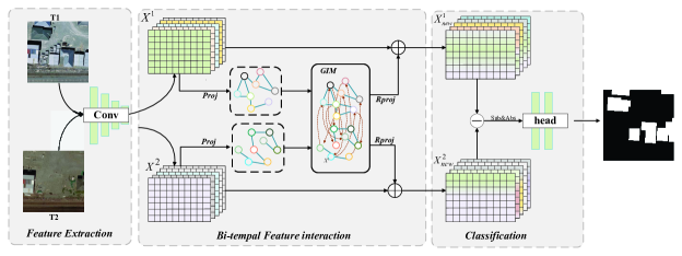
Figure 1 illustrates the architecture of the proposed BGINet. The network comprises two main components: a generic feature extractor and a Bitemporal Graph Interaction Module. To ensure model efficiency, we utilize the first three stages of ResNet-18 [15] as the generic feature extractor. The Graph Interaction Module (GIM) branch takes the bitemporal generic features extracted by the feature extractor as input and maps them into a graph structure. Inspired by nonlocal operations, we incorporate self-attentiveness in the graph space to efficiently capture remote dependencies between bitemporal features. The evolved bitemporal features are then integrated with the original features. Finally, a 1 × 1 convolutional layer with a sigmoid activation function is applied to obtain the final difference map, which serves as an indicator of change.

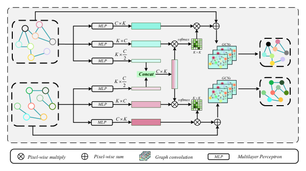
Here, we detail the Graph Interaction Module (GIM). As shown in Figure 2, GIM are composed of three operations, namely, graph projection, graph interaction, and graph reprojection. Given bitemporal 2D feature map $X^{1}\in\mathbb{R}^{h\times w\times c}$,$X^{2}\in\mathbb{R}^{h\times w\times c}$ , $\boldsymbol{x}_{ij}^{1}$,$\boldsymbol{x}_{ij}^{2}\in\mathbb{R}^{d}$ denotes the d-dimensional feature at $(i,j)$of bitemporal. The graph embedding can be denoted as $\mathcal{G}_{1}=(\mathcal{V}_{1},\mathcal{Z}_{1},\mathcal{A}_{1})$ or $\mathcal{G}_{2}=(\mathcal{V}_{2},\mathcal{Z}_{2},\mathcal{A}_{2})$, where ${\mathcal{V}_{1}}$,${\mathcal{V}_{2}}$ is a set of nodes, ${\mathcal{Z}_{1}}$,${\mathcal{Z}_{2}}$ is the feature matrix, and ${\mathcal{A}_{1}}$,${\mathcal{A}_{2}}$ is the affinity matrix between the nodes.

1) Graph Projection: To establish a correspondence between maps $X^{1}$ and $X^{2}$, we perform a feature mapping to obtain graphs $\mathcal{G}_{1}$ and $\mathcal{G}_{2}$. In this mapping, pixels with similar features are assigned to the same vertex in the graph. For simplicity, let’s consider the feature mapping of the $t_{1}$ time phase as an example. Following the approach in [14], we parameterize two matrices $\mathcal{W}\in\mathbb{R}^{|\mathcal{V}|\times d}$ and $\Sigma\in\mathbb{R}^{|\mathcal{V}|\times d}$, where $|\mathcal{V}|$ represents the number of vertices, which can be pre-specified.

Each row $w_{k}$ of $\mathcal{W}$ serves as the anchor point for vertex $k$. To compute the soft assignment $q_{ij}^{k}$ of feature vector $\boldsymbol{x}_{ij}$ to $w_{k}$, we use the following equation:

In this equation, $\sigma_{k}$ is the row vector of $\Sigma$ and is constrained to the range $(0,1)$ using a sigmoid function. The numerator measures the similarity between the feature vector and the anchor point, while the denominator normalizes the assignment across all vertices. Next, we encode the vertex feature matrix $\mathcal{Z}\in R^{|\mathcal{V}|\times d}$ using the corresponding pixel features. For vertex $k$, we compute $z_{k}$, which represents the weighted average of the residuals between feature vectors $x_{ij}$ and $w_{k}$. Then, we normalize $z_{k}$ to obtain $z^{\prime}_{k}$, the unit vector that forms the row vector of the feature matrix $\mathcal{Z}$ of graph $\mathcal{G}$:

Finally, the graph affinity matrix $\mathcal{A}$ is computed using the equation:

2) Graph Interaction: The proposed GIM receiver map embeddings $\mathcal{G}_{1}=(\mathcal{V}_{1},\mathcal{Z}_{1},\mathcal{A}_{1})$, and $\mathcal{G}_{2}=(\mathcal{V}_{2},\mathcal{Z}_{2},\mathcal{A}_{2})$ as inputs form the feature mapping of $t_{1}$ time phase and $t_{2}$ time phase, respectively, and models the between graph interaction and guides the inter-graph message passing from $V_{1}$ to $V_{2}$ and $V_{2}$ to $V_{1}$. This goal leads us to take inspiration from non-local operations and DMINet [51] and compute inter-graph dependencies with a concern mechanism. This operation of ours significantly reduces the number and computational complexity of parameters and achieves better results

GIM models the betweengraph interaction and guides the inter-graph message passing from $\mathcal{Z}_{1}$ to $\mathcal{Z}_{2}$ or from $\mathcal{Z}_{2}$ to $\mathcal{Z}_{1}$ As shown in Figure3,we use different multi-layer perceptrons (MLPs) to transform $\mathcal{Z}_{1}$ to the query graph $\mathcal{Z}_{1}^{q}$,key graph $\mathcal{Z}_{1}^{k}$ and value graph $\mathcal{Z}_{1}^{v}$ transform $\mathcal{Z}_{2}$ to the query graph $\mathcal{Z}_{2}^{q}$,key graph $\mathcal{Z}_{2}^{k}$ and value $\mathcal{Z}_{2}^{v}$.Next, we unify $\mathcal{Z}_{1}^{q}$,$\mathcal{Z}_{2}^{q}$ as:

Then, the similarity matrix $\mathcal{A}_{1\rightarrow 2}^{\text{inter }}$ and $\mathcal{A}_{2\rightarrow 1}^{\text{inter }}$$\in\mathbb{R}^{K\times K}$is calculated by a matrix multiplication as:

where $\mathcal{A}_{C\rightarrow E}^{\text{inter }}\in\mathbb{R}^{K\times K}$. After that, we can transfer semantic information from $\mathcal{Z}_{1}$ to $\mathcal{Z}_{2}$ and $\mathcal{Z}_{2}$ to $\mathcal{Z}_{1}$ by

After performing inter-graph interaction, we conduct the intra-graph reasoning by taking$\mathcal{Z}_{1}^{\prime}$ and $\mathcal{Z}_{2}^{\prime}$ as inputs to obtain enhanced graph representations.

3) Graph Reprojection: To map the enhanced graph representations back to the original coordinate space, we revisit the assignments from the graph projection step.

The WHU Building Change Detection Dataset[16]:The data consists of two aerial images of two different time phases and the exact location, which contains 12796 buildings in 20.5 km2 with a resolution of 0.2 m and a size of 32570x15354. We crop the images to 256x256 size and randomly divide the training, validation, and test sets: 6096/762/762.

Guangzhou Dataset(GZ-CD)[17]: The dataset was collected from 2006-2019, covering the suburbs of Guangzhou, China, and to facilitate the generation of image pairs, the Google Earth service of BIGEMAP software was used to collect 19 seasonally varying VHR image pairs with a spatial resolution of 0.55 m and a size range of 1006x1168 pixels to 4936x5224.We crop the images to 256x256 size and randomly divide the training, validation, and test sets: 2876/353/374.

In the experiment, the number of vertices $|\mathcal{V}|$ is set to 32. We utilize the AdamW optimizer with weight decay 1e-4 and a polynomial schedule, where the initial learning rate is set to 0.0004. The total number of iterations is set to 100. The GPU used for the experiment is an NVIDIA V100.In this experiment, we employ the joint loss function consisting of Focal loss and Dice loss. For Focal loss, we set the parameters $\gamma$ and $\alpha$ to 2.0 and 0.2, respectively.The overall loss function is formulated as follows:

Here, $\sigma$ represents the sigmoid activation function. We denote the model prediction as $p$, and $\lambda_{1}$ and $\lambda_{2}$ as the coefficients of the Focal loss and Dice loss, respectively. In this experiment, we set $\lambda_{1}$ and $\lambda_{2}$ to 0.5 and 1, respectively.

Our comparison experiments evaluate the trade-off between accuracy, number of parameters, and floating-point operations (FLOP). The quantitative results for the two datasets are presented in Table I and Table II, respectively. The best-performing model in each column is highlighted in bold, while the second-best model is underlined. The tables provide a comprehensive view of the performance metrics, allowing us to analyze the accuracy and efficiency of different models

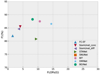
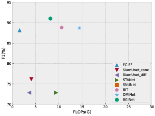
In Fig. 3 and Fig. 4, we present a tradeoff analysis between the F1 score and computational cost for various classical remote sensing image change detection methods and recently proposed methods (e.g., STANet, BIT, DMINet, etc.). These figures provide valuable insights into different approaches’ performance and computational requirements.The results indicate that while the aforementioned methods demonstrate good performance, they often have a significant computational overhead. On the other hand, baseline models like FC-EF require minimal computational resources but fall short in accuracy. Our proposed method, however, achieves a favorable balance between accuracy and computational overhead.By examining the figures, it is evident that our method outperforms the baseline models in terms of accuracy while still maintaining a manageable computational cost. This highlights the effectiveness and efficiency of our approach in remote sensing image change detection tasks.

To validate the effectiveness of our proposed BGINet, we conducted ablation experiments on network knots using two publicly available datasets. The results of these experiments are presented in Table 3. As a baseline model, we selected resnet18 and utilized only the first three stages of the network. Upon introducing GIM (Graph Interaction Module) on the GZ-CD dataset, we observed improved precision, recall, and F1 scores by $1.05\%,2.63\%,and1.84\%$, respectively. On the WHU dataset, although there was a decrease in the recall by $2.02\%$, we observed improvements in precision and F1 scores by $6.14\%$ and $2.2\%$, respectively. These findings highlight the positive impact of our proposed BGINet, particularly when integrated with GIM, in enhancing the performance of remote sensing image change detection. The ablation experiments demonstrate the introduced graph interaction module’s significance and contribution to improving precision, recall, and overall F1 score on both datasets. Overall, the results affirm the effectiveness of our approach and its potential for advancing the field of remote sensing image change detection.

References

- [1] M. Liu, Z. Chai, H. Deng, and R. Liu, “A cnn-transformer network with multiscale context aggregation for fine-grained cropland change detection,” IEEE Journal of Selected Topics in Applied Earth Observations and Remote Sensing, vol. 15, pp. 4297–4306, 2022, doi:10.1109/JSTARS.2022.3177235.
- [2] H. Chen, Z. Qi, and Z. Shi, “Remote sensing image change detection with transformers,” IEEE Transactions on Geoscience and Remote Sensing, vol. 60, pp. 1–14, 2022, doi:10.1109/TGRS.2021.3095166.
- [3] T. Celik, “Unsupervised change detection in satellite images using principal component analysis and -means clustering,” IEEE Geoscience and Remote Sensing Letters, vol. 6, no. 4, pp. 772–776, 2009, doi:10.1109/LGRS.2009.2025059.
- [4] N. Zerrouki, F. Harrou, and Y. Sun, “Statistical monitoring of changes to land cover,” IEEE Geoscience and Remote Sensing Letters, vol. 15, no. 6, pp. 927–931, 2018, doi:10.1109/LGRS.2018.2817522.
- [5] S. Fang, K. Li, J. Shao, and Z. Li, “Snunet-cd: A densely connected siamese network for change detection of vhr images,” IEEE Geoscience and Remote Sensing Letters, vol. 19, pp. 1–5, 2022, doi:10.1109/LGRS.2021.3056416.
- [6] H. Chen, F. Pu, R. Yang, R. Tang, and X. Xu, “Rdp-net: Region detail preserving network for change detection,” IEEE Transactions on Geoscience and Remote Sensing, vol. 60, pp. 1–10, 2022, doi:10.1109/TGRS.2022.3227098.
- [7] J. Hu, L. Shen, and G. Sun, “Squeeze-and-excitation networks,” in Proceedings of the IEEE conference on computer vision and pattern recognition, 2018, pp. 7132–7141.
- [8] S. Woo, J. Park, J.-Y. Lee, and I. S. Kweon, “Cbam: Convolutional block attention module,” in Proceedings of the European conference on computer vision (ECCV), 2018, pp. 3–19.
- [9] M. Liu, Z. Chai, H. Deng, and R. Liu, “A cnn-transformer network with multiscale context aggregation for fine-grained cropland change detection,” IEEE Journal of Selected Topics in Applied Earth Observations and Remote Sensing, vol. 15, pp. 4297–4306, 2022, doi:10.1109/JSTARS.2022.3177235.
- [10] A. Abuelgasim, W. Ross, S. Gopal, and C. Woodcock, “Change detection using adaptive fuzzy neural networks: Environmental damage assessment after the gulf war,” Remote Sensing of Environment, 1999.
- [11] A. Frick and S. Tervooren, “A framework for the long-term monitoring of urban green volume based on multi-temporal and multi-sensoral remote sensing data,” Journal of geovisualization and spatial analysis, vol. 3, no. 1, p. 6, 2019.
- [12] A. Vaswani, N. Shazeer, N. Parmar, J. Uszkoreit, L. Jones, A. N. Gomez, Ł. Kaiser, and I. Polosukhin, “Attention is all you need,” Advances in neural information processing systems, vol. 30, 2017.
- [13] Y. Feng, J. Jiang, H. Xu, and J. Zheng, “Change detection on remote sensing images using dual-branch multilevel intertemporal network,” IEEE Transactions on Geoscience and Remote Sensing, vol. 61, pp. 1–15, 2023.
- [14] Y. Li and A. Gupta, “Beyond grids: Learning graph representations for visual recognition,” in Neural Information Processing Systems, 2018.
- [15] K. He, X. Zhang, S. Ren, and J. Sun, “Deep residual learning for image recognition,” in Proceedings of the IEEE conference on computer vision and pattern recognition, 2016, pp. 770–778.
- [16] S. Ji, S. Wei, and M. Lu, “Fully convolutional networks for multisource building extraction from an open aerial and satellite imagery data set,” IEEE Transactions on geoscience and remote sensing, vol. 57, no. 1, pp. 574–586, 2018.
- [17] D. Peng, L. Bruzzone, Y. Zhang, H. Guan, H. Ding, and X. Huang, “Semicdnet: A semisupervised convolutional neural network for change detection in high resolution remote-sensing images,” IEEE Transactions on Geoscience and Remote Sensing, vol. 59, no. 7, pp. 5891–5906, 2021, doi:10.1109/TGRS.2020.3011913.
- [18] H. Chen and Z. Shi, “A spatial-temporal attention-based method and a new dataset for remote sensing image change detection,” Remote Sensing, vol. 12, no. 10, 2020, doi:10.3390/rs12101662. [Online]. Available: https://www.mdpi.com/2072-4292/12/10/1662
- [19] R. Caye Daudt, B. Le Saux, and A. Boulch, “Fully convolutional siamese networks for change detection,” in 2018 25th IEEE International Conference on Image Processing (ICIP), 2018, pp. 4063–4067, doi:10.1109/ICIP.2018.8451652.