Robot Deformable Object Manipulation via NMPC-generated Demonstrations in Deep Reinforcement Learning

For a square piece of fabric as a representative deformable object, these tasks are designed: folding along the diagonal, folding along the central axis, and flattening. In each task, the robot is allowed a maximum number of operations, denoted as $t_{\text{m}}$, which varies among different tasks. At the beginning of each experimental round, the robot returns to its default initial pose, while the initial position of the fabric is set according to the requirements of the specific task and is subject to a certain degree of random noise. The details are as followed:

• •

  Folding along the diagonal: The specific objective of the operation is to achieve perfect alignment of one pair of diagonal endpoints of the fabric, while maintaining the distance between the other pair of diagonal endpoints exactly equal to the length of the fabric diagonal, and ensuring that the area of the fabric is equal to half of its area when fully unfolded.

• •

  Folding along the central axis: Before folding, the two sets of fabric endpoints should be symmetrically arranged relative to the folding axis. After folding, these two sets of endpoints should coincide, while ensuring that the distance between endpoints on the side of the folding axis remains consistent with before folding, and the area of the fabric is equal to half of its area when fully unfolded.

• •

  Flattening: When faced with heavily wrinkled fabric, the robot’s task is to flatten it to its maximum area. At the beginning of each experiment, the fabric is initialized by the robot applying random actions within the first 10 time steps. The robot moves a point on the fabric from its initial position to a placement point within a distance of 0.1 m to 0.2 m during each random step, ensuring sufficient disturbance to generate random wrinkles.

Previous studies [21, 30] often directly fed the visual information of the scene as state inputs to DRL, which is intuitive but results in an overly complex state space. Some research [22] simplifies the state space in simulation by using the coordinates of deformable object feature points as state inputs, which is simple but difficult to directly transfer to the real world. This article adopts a compromise solution. Algorithms from OpenCV are utilized to preprocess the visual information of the scene, and the processed results are then used as state inputs for DRL. The state spaces of three different tasks are introduced as follows.

In both the along-diagonal and along-axis folding tasks, using Canny edge detection [31] and the Douglas-Peucker algorithm in OpenCV, the four right-angle corners of the fabric can be identified. During robot manipulation, considering the relationship between the fabric’s motion speed and the robot’s operation speed, this article, under the premise of relatively slow robot operation, employs the pyramid Lucas-Kanade optical flow tracking method to track the four corners. This article selects the positions of the four corners of the square fabric and the proportion $f_{t}$ of the fabric’s current area to its area when fully flattened as the state representation in these two folding tasks. This results in a 13-dimensional state space, as shown in Fig. 2(a). The symbols defining the state variables for the folding tasks are as follows:

where $\boldsymbol{p}_{1_{t}},\boldsymbol{p}_{2_{t}},\boldsymbol{p}_{3_{t}},\boldsymbol{p}_{4_{t}}$ respectively represent the three-dimensional coordinates of the four corners of the fabric at time $t$. All coordinates and vectors mentioned in this article are described with respect to the base coordinate system of the robot they are associated with.

In the flattening task, the fabric’s initial state is heavily wrinkled, making it extremely difficult to detect the right-angle corners of the fabric. We use Canny edge detection and the Douglas-Peucker algorithm in OpenCV to fit the contour of the fabric into an octagon, representing the eight points on the contour that best characterize the shape of the fabric. The coordinates of the eight endpoints, the coordinates of the center point of the fabric contour and the proportion of the fabric’s current area to its area when fully flattened are the state representation. Ultimately, the dimensionality of the state space used in the spreading task in this article is 28, as shown in Fig. 2(b). The symbols defining the state variables for the spreading task are as follows:

where $\boldsymbol{p}_{1_{t}},\boldsymbol{p}_{2_{t}},\cdots,\boldsymbol{p}_{8_{t}}$ respectively represent the three-dimensional coordinates of the eight fitted endpoints of the fabric at time $t$, and $\boldsymbol{p}_{\text{c}_{t}}$ represents the three-dimensional coordinates of the center point of the fabric contour at time $t$.

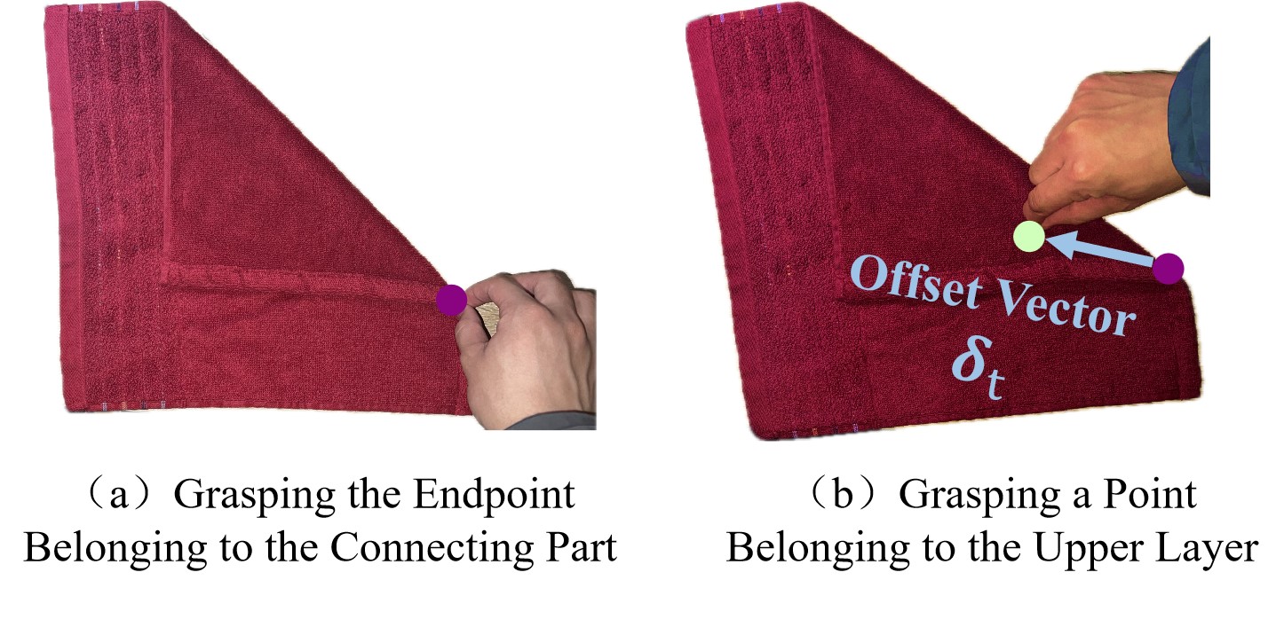
During the process of collecting human demonstrations, we found that humans only need to manipulate the four endpoints of the fabric to complete all folding tasks. In contrast, a strategy solely based on manipulating the endpoints of the fabric outline has minimal effect in flattening tasks. Fig. S1 explains this phenomenon: the fabric in a folded state is divided into upper layer (green), intermediate connecting parts (purple), and lower layer (orange), as shown in Fig. S2(a). Effective relative displacement between the upper and lower layers occurs only when manipulating points on the upper layer, as depicted in Fig. S2(b). Conversely, manipulating the lower layer or the connecting parts, as shown in Fig. S2(c), mostly results in overall movement of the fabric, which is not substantially helpful for flattening tasks.

This article designs a motion vector, as illustrated in Fig. 3. An offset vector $\boldsymbol{\delta}_{t}$ is introduced based on the fabric’s edge endpoints to enable the robot to grasp points on the upper layer of the fabric. By adjusting $\boldsymbol{\delta}_{t}$, the robot can grasp any part of the fabric to manipulate it.

This article refines the operation process into three key steps: firstly, selecting one endpoint from the state variables as the base grasping point; secondly, generating an offset vector $\boldsymbol{\delta}_{t}$ to accurately adjust the position of the grasping point; thirdly, determining the coordinates of the placement point to guide the robot to complete the entire action from grasping to placing. The representation of the action space is described in (3):

where $p_{\text{g}_{t}}$ represents the index of the endpoint selected at time $t$ in the state variables, $\boldsymbol{\delta}_{t}$ represents the offset vector for time $t$, and $\boldsymbol{p}_{\text{p}_{t}}$ represents the coordinates of the placement point at time $t$.

The state transition from time $t$ to time $t+1$ is controlled by $\boldsymbol{a}_{t}$ as expressed in (3). Initially, the robot determines the coordinates of the corresponding endpoint $\boldsymbol{p}_{\text{g}_{t}}$ in $\boldsymbol{s}_{t}$ based on $p_{\text{g}_{t}}$. Subsequently, by combining $\boldsymbol{\delta}_{t}$, the actual grasping coordinates $\boldsymbol{g}_{t}=\boldsymbol{p}_{\text{g}_{t}}+\boldsymbol{\delta}_{t}$ are calculated, guiding the end effector to execute the grasping action at the $\boldsymbol{g}_{t}$ position. Finally, the robot moves the end effector to the $\boldsymbol{p}_{\text{p}_{t}}$ position, opens the gripper, and completes the placing operation.

In the diagonal folding task, as shown in Fig. 2, the target state of the fabric is when endpoint 1 and endpoint 3 coincide, and the distance between endpoint 2 and endpoint 4 equals the length of the diagonal, with the unfolded area of the fabric equal to half of its fully unfolded area. Assuming the side length of the square fabric is $l_{s}$, we define the difference $e_{t}$ between the fabric state at time $t$ and the target state in the diagonal folding task as follows:

The objective of folding along the central axis is to align endpoint 1 with endpoint 2, endpoint 3 with endpoint 4, ensure that the distance between endpoint 1 and endpoint 3 equals the distance between endpoint 2 and endpoint 4, both equal to ls, and the fabric’s unfolded area equals half of its fully unfolded area. We define the gap $e_{t}$ between the fabric state at time $t$ and the target state in the folding along the central axis task as follows:

For $e_{t}$ in different folding tasks, we define their reward functions as follows:

where $done$ represents the completion status of the task, which becomes True when the maximum number of operations, $t_{\text{m}}$, is reached. $t_{\text{z}}$ is the threshold to measure whether the fabric state has significantly changed. According to (6), the reward mechanism $r(\boldsymbol{s}_{t},\boldsymbol{a}_{t})$ assigns rewards or penalties to the agent based on its immediate actions and states, following the following guidelines:

• •

  At the end of a round, a decisive reward of $-200e_{t}+100$ is given based on the error $e_{t}$. The greater the error, the lower the decisive reward. The decisive reward is set to 100 when the $e_{t}$ is 0.

• •

  If the round is not over and the error significantly decreases, i.e., $e_{t-1}-e_{t}>t_{\text{z}}$, indicating the agent is approaching the target, a positive reward of 3 is given to encourage similar behavior.

• •

  Conversely, if the round is not over and the error significantly increases, i.e., $e_{t}-e_{t-1}>t_{\text{z}}$, indicating the agent deviates from the target, a negative penalty of -3 is applied to suppress this behavior.

In the flattening task, we directly define the reward function for the flattening task based on the ratio $f_{t}$ of the fabric’s unfolded area at time $t$ to its fully unfolded area:

The criteria followed here are similar to those described in (6), and will not be repeated here.

In this article, as long as a suitable final $\boldsymbol{p}_{\text{p}_{t}}$ is chosen, selecting any reference $p_{\text{g}_{t}}$ can promote the task to some extent. Therefore, the selection of the fabric $p_{\text{g}_{t}}$ is more closely related to the application range of fuzzy sets. We use the state-action pairs $(\boldsymbol{s}_{t},\boldsymbol{a}_{t})$, with the state $\boldsymbol{s}_{t}$ as input and $p_{\text{g}_{t}}$ from the action $\boldsymbol{a}_{t}$ as output, to construct an HTSK fuzzy system, denoted as $H(\boldsymbol{s}_{t};\boldsymbol{\theta}^{h})$, where $\boldsymbol{\theta}^{h}$ represents its parameters. The input-output relationship of $H(\boldsymbol{s}_{t};\boldsymbol{\theta}^{h})$ is represented as follows:

The training data for the selection strategy of the reference grasping point is sourced from the human demonstration dataset $\mathcal{D}_{\text{demo}}$. Additionally, data with significant contributions to task progress are continuously supplemented during the interaction between the robot and the environment, denoted as $\mathcal{D}_{\text{grasp}}=(\boldsymbol{s}_{n},p_{\text{g}_{n}})^{N}_{n=1}$, where $N$ is the size of the training dataset, $\boldsymbol{s}_{n}=({s}_{1}^{(n)},s_{2}^{(n)},\ldots,s_{M}^{(n)})$ represents the $M$-dimensional state variables of the $n$-th sample, $p_{\text{g}_{n}}\in(1,2,\cdots,k)$ is the index of the reference grasping point for the $n$-th sample, which is also the label of the training dataset, and $k$ is the number of candidate reference grasping points. The system learns the mapping relationship between the states $\boldsymbol{s}_{n}$ and the corresponding reference grasping points $p_{\text{g}_{n}}$ in the demonstration dataset, enabling it to predict appropriate reference grasping points under different states.

The primary improvement of HTSK over TSK is reflected in the saturation issues related to the dimensions of the data. In TSK fuzzy systems, the traditional softmax function is used to calculate the normalized firing levels $\overline{\omega}_{r}$ of each fuzzy rule, as follows:

Here, $H_{r}$ decreases as the dimension $M$ of the input data increases, leading to the saturation of the softmax function [28]. In conventional TSK fuzzy systems, typically only the fuzzy rule with the highest $H_{r}$ receives a non-zero firing level $\overline{\omega}_{r}$. Consequently, as the data dimension $M$ increases, the distinctiveness of all $H_{r}$ values diminishes, and the classification performance of the TSK fuzzy system declines. To address this saturation issue, HTSK substitutes $H_{r}$ in the normalized firing levels $\overline{\omega}_{r}$ of each fuzzy rule within the TSK system with its mean value $H_{r}^{*}$, thereby allowing the normalization process to better accommodate high-dimensional data inputs. In the sixth and seventh layers of the HTSK net [29], based on the softmax function and the probability distribution, the final $p_{\text{g}_{t}}$ is selected as the output.

This article adopts the k-means clustering method to initialize $c_{r,m}$ which is the parameter of the Gaussian membership function, the cross-entropy loss function to measure the difference between the output of the fuzzy system and the true labels, and the Adam optimizer for gradient descent, with a learning rate of 0.04, a batch size of 64, and a weight decay of 1e-8.

In Rainbow-DDPG, BC is typically implemented by adding $L_{\text{bc}}$ to the loss function of the Actor network, as shown in (19):

The definition of $L_{\text{bc}}$ only takes effect when $Q(\boldsymbol{s}_{i},\boldsymbol{a}_{i};\boldsymbol{\varphi})>Q(\boldsymbol{s}_{i},\mu(\boldsymbol{s}_{i};\boldsymbol{\theta});\boldsymbol{\varphi})$. However, training the Critic network to output accurate Q-values is a time-consuming process, which results in the ineffectiveness of $L_{\text{bc}}$ in the early stages of training. Additionally, when the Critic network is fully trained, the replay buffer mainly contains real-time interaction data rather than demonstration data, reducing the probability of sampling demonstration data for training. Therefore, $L_{\text{bc}}$ may not have a significant impact, and RL still requires considerable training time to achieve good policies.

We propose GABC to improve Rainbow-DDPG for generating $\boldsymbol{\delta}_{t}$ and $\boldsymbol{p}_{\text{p}_{t}}$. We denote the current Actor network as $\mu(\boldsymbol{s}_{t},p_{\text{g}_{t}};\boldsymbol{\theta}^{\mu})$, where $\boldsymbol{\theta}^{\mu}$ represents its parameters. In each state $\boldsymbol{s}_{t}$, this network combines with environmental noise $\mathcal{N}(0,\sigma^{2})$ to output $\boldsymbol{\delta}_{t}$ and $\boldsymbol{p}_{\text{p}_{t}}$, guiding the robot to perform fabric manipulation tasks. The input-output relationship of $\mu(\boldsymbol{s}_{t},p_{\text{g}_{t}};\boldsymbol{\theta}^{\mu})$ is represented as follows:

Its current Critic network is denoted as $Q(\boldsymbol{s}_{t},\boldsymbol{a}_{t};\boldsymbol{\theta}^{q})$, where $\boldsymbol{\theta}^{q}$ represents its parameters. In each state $\boldsymbol{s}_{t}$, this network outputs a Q-value $Q(\boldsymbol{s}_{t},\boldsymbol{a}_{t};\boldsymbol{\theta}^{q})$ through $\boldsymbol{\theta}^{q}$ to evaluate the quality of action $\boldsymbol{a}_{t}$. Since the quality of $\boldsymbol{\delta}_{t}$ and $\boldsymbol{p}_{\text{p}_{t}}$ is closely related to the selection of $p_{\text{g}_{t}}$, the input $\boldsymbol{a}_{t}$ of $Q(\boldsymbol{s}_{t},\boldsymbol{a}_{t};\boldsymbol{\theta}^{q})$ not only includes $\boldsymbol{\delta}_{t}$ and $\boldsymbol{p}_{\text{p}_{t}}$ output by the Actor network but also includes $p_{\text{g}_{t}}$ output from demonstration data or the $H(\boldsymbol{s}_{t};\boldsymbol{\theta}^{h})$.

Assuming that during training, the sampled state-action data pairs are $(\boldsymbol{s}_{i},\boldsymbol{a}_{i})$, where $\boldsymbol{a}_{i}=(p_{\text{g}_{i}},\boldsymbol{\delta}_{i},\boldsymbol{p}_{\text{p}_{i}})$. This study denotes $(\boldsymbol{\delta}_{i},\boldsymbol{p}_{\text{p}_{i}})$ as $\boldsymbol{b}_{i}$, and sets $\boldsymbol{w}_{i}=(p_{\text{g}_{i}},\mu(\boldsymbol{s}_{i},p_{\text{g}_{i}};\boldsymbol{\theta}^{\mu}))$. Then, in the framework of this article, $L_{\text{bc}}$ can be redefined as follows:

To expedite the training of the Critic, GABC introduces a loss term called $Q_{\text{diff}}$ into the current Critic network’s loss function. Assuming $(\boldsymbol{s}_{i},\boldsymbol{a}_{i})\in\mathcal{D}_{\text{demo}}$, based on the fact that $\boldsymbol{\delta}_{i}$ and the placement point $\boldsymbol{p}_{\text{p}_{i}}$ in the human demonstration actions $\boldsymbol{a}_{i}$ are significantly superior to the offset vector and placement point output by the current Actor network $\mu(\boldsymbol{s}_{i},p_{\text{g}_{i}};\boldsymbol{\theta}^{\mu})$, $Q_{\text{diff}}$ guides the training of the Critic network by measuring the difference between the $Q$-values output by the current Critic network for the actions $\boldsymbol{a}_{i}$ in the human demonstration data and the $Q$-values output for the actions $\boldsymbol{w}_{i}=(p_{\text{g}_{i}},\mu(\boldsymbol{s}_{i},p_{\text{g}_{i}};\boldsymbol{\theta}^{\mu}))$ by the current Actor network, under the same state $\boldsymbol{s}_{i}$. Specifically, this article sets a pre-training stage, during which, in the pre-training phase, when $Q(\boldsymbol{s}_{i},\boldsymbol{a}_{i};\boldsymbol{\theta}^{q})-Q(\boldsymbol{s}_{i},\boldsymbol{w}_{i};\boldsymbol{\theta}^{q})\geq 100$, $Q_{\text{diff}}$ is set to 0; otherwise, $Q_{\text{diff}}=100-(Q(\boldsymbol{s}_{i},\boldsymbol{a}_{i};\boldsymbol{\theta}^{q})-Q(\boldsymbol{s}_{i},\boldsymbol{w}_{i};\boldsymbol{\theta}^{q}))$, as shown in (22):

After pre-training is completed, the Actor network has already acquired a certain policy, and its output actions $\mu(\boldsymbol{s}_{i},p_{\text{g}_{i}};\boldsymbol{\theta}^{\mu})$ may not significantly inferior to the actions $\boldsymbol{a}_{i}$ in the human demonstration data. The introduction of $Q_{\text{diff}}$ may lead to the training of the Actor network getting stuck in local optima, so that the $Q_{\text{diff}}$ is removed.

The loss function $L_{\text{Critic}}$ for the improved Critic network $Q(\boldsymbol{s}_{t},\boldsymbol{a}_{t};\boldsymbol{\theta}^{q})$ is defined as follows:

where $\lambda_{\text{1step}}$ and $\lambda_{n\text{step}}$ are the weights of the 1-step and n-step TD loss functions, respectively. $\lambda_{\text{diff}}$ is the weight of $Q_{\text{diff}}$, set to 1 during the pre-training phase and 0 in subsequent phases. $L_{\text{1s}}$ and $L_{n\text{s}}$ are similar to the 1-step and n-step TD loss functions [21], and the target functions $y_{\text{1s}}$ and $y_{n\text{s}}$ can be referenced from TD3 model [32]. Here, we define $Q^{\prime}_{1}$, $Q^{\prime}_{2}$, and $\mu^{\prime}$ as two target Critic networks and one target Actor network, with $\boldsymbol{w}^{\prime}_{i+k}=(H(\boldsymbol{s}_{i+k};\boldsymbol{\theta}^{h}),\mu^{\prime}(\boldsymbol{s}_{i+k},H(\boldsymbol{s}_{i+k};\boldsymbol{\theta}^{h});\boldsymbol{\theta}^{{\mu}^{\prime}})),k=1,2,\cdots,n,$ where $n$ is the step length of the n-step TD loss function, $N$ is the batch size, $r_{i}$ is the reward, and $\gamma$ is the discount factor. Consequently, $L_{\text{1s}}$ and $L_{\text{ns}}$ are defined as follows:

During training, the introduction of $Q_{\text{diff}}$ causes the current Critic network to initially tend towards generating larger $Q$-values for actions $\boldsymbol{a}_{i}$ from human demonstrations, the effect of $L_{\text{bc}}$ in (21) becomes more pronounced, leading to a more thorough utilization of human demonstrations and thus accelerating the training of the Actor network. Additionally, the training of the current Actor network $\mu(\boldsymbol{s}_{i},p_{\text{g}_{i}};\boldsymbol{\theta}^{\mu})$ also depends on the $Q$-values output by the current Critic network $\mu(\boldsymbol{s}_{t},p_{\text{g}_{t}};\boldsymbol{\theta}^{\mu})$. Consequently, a current Critic network capable of providing more precise $Q$-values will further accelerate the training of the current Actor network.

This article adopts the CPL training method illustrated in Fig. 5. At each state $\boldsymbol{s}_{t}$, CPL first utilizes the $H(\boldsymbol{s}_{t};\boldsymbol{\theta}^{h})$ to select $p_{\text{g}_{t}}$, and then, based on $p_{\text{g}_{t}}$, selects $\boldsymbol{\delta}_{t}$ and $\boldsymbol{p}_{\text{p}_{t}}$ through $\mu(\boldsymbol{s}_{t},p_{\text{g}_{t}};\boldsymbol{\theta}^{\mu})$.

CPL often faces the challenge of loss allocation [30]. It’s difficult to determine whether high rewards obtained for an action are attributed to the grasping policy $H(\boldsymbol{s}_{t};\boldsymbol{\theta}^{h})$ or the offset vector and placement point selection policy $\mu(\boldsymbol{s}_{t},p_{\text{g}_{t}};\boldsymbol{\theta}^{\mu})$. To address this, the following training approach is adopted. Firstly, each state-action pair $(\boldsymbol{s}_{t},\boldsymbol{a}_{t})$ is extracted from $\mathcal{D}_{\text{demo}}$ to form an initial training dataset $\mathcal{D}_{\text{grasp}}$ tailored for the HTSK fuzzy system. Then, $\mathcal{D}_{\text{grasp}}$ is used to train $H(\boldsymbol{s}_{t};\boldsymbol{\theta}^{h})$ to get $\boldsymbol{\theta}^{h}$. Subsequently, with $\boldsymbol{\theta}^{h}$ fixed, based on the $H(\boldsymbol{s}_{t};\boldsymbol{\theta}^{h})$ to select $p_{\text{g}_{t}}$, the improved Rainbow-DDPG algorithm with GABC enhancement is employed to train the offset vector and placement point selection policy $\mu(\boldsymbol{s}_{t},p_{\text{g}_{t}};\boldsymbol{\theta}^{\mu})$, obtaining $\boldsymbol{\theta}^{\mu}$.

During the process, data is also collected to supplement the training dataset $\mathcal{D}_{\text{grasp}}$ and continuously train the improved grasping policy $H(\boldsymbol{s}_{t};\boldsymbol{\theta}^{h})$ parameters $\boldsymbol{\theta}^{h}$. Specifically, when the action $\boldsymbol{a}_{t}$ executed by the robot at time $t$ significantly advances the progress of the task (in folding tasks, $e_{t-1}-e_{t}>t_{\text{z}}$, in flattening tasks, $f_{t}-f_{t-1}>t_{\text{z}}$), $(\boldsymbol{s}_{t},\boldsymbol{a}_{t})$ is added to $\mathcal{D}_{\text{grasp}}$. After getting a certain amount of new data, $\mathcal{D}_{\text{grasp}}$ is used to retrain the grasping policy $H(\boldsymbol{s}_{t};\boldsymbol{\theta}^{h})$ to get new parameters $\boldsymbol{\theta}^{h}$.

Combining all the improvements introduced above, we proposed the HGCR-DDPG algorithm. The relevant pseudocode is detailed in Algorithm 1.

References

- [1] J. Zhu et al., “Challenges and Outlook in Robotic Manipulation of Deformable Objects,” in IEEE Robotics & Automation Magazine, vol. 29, no. 3, pp. 67-77, Sept. 2022.
- [2] P. Long, W. Khalil and P. Martinet, “Modeling & control of a meat-cutting robotic cell,” 2013 16th International Conference on Advanced Robotics (ICAR), Montevideo, Uruguay, 2013, pp. 1-6.
- [3] M. C. Gemici and A. Saxena, “Learning haptic representation for manipulating deformable food objects,” 2014 IEEE/RSJ International Conference on Intelligent Robots and Systems, Chicago, IL, USA, 2014, pp. 638-645.
- [4] I. Leizea, A. Mendizabal, H. Alvarez, I. Aguinaga, D. Borro and E. Sanchez, “Real-Time Visual Tracking of Deformable Objects in Robot-Assisted Surgery,” in IEEE Computer Graphics and Applications, vol. 37, no. 1, pp. 56-68, Jan.-Feb. 2017.
- [5] B. Thananjeyan, A. Garg, S. Krishnan, C. Chen, L. Miller and K. Goldberg, “Multilateral surgical pattern cutting in 2D orthotropic gauze with deep reinforcement learning policies for tensioning,” 2017 IEEE International Conference on Robotics and Automation (ICRA), Singapore, 2017, pp. 2371-2378.
- [6] Y. Gao, H. J. Chang and Y. Demiris, “Iterative path optimisation for personalised dressing assistance using vision and force information,” 2016 IEEE/RSJ International Conference on Intelligent Robots and Systems (IROS), Daejeon, Korea (South), 2016, pp. 4398-4403.
- [7] F. Zhang and Y. Demiris, “Learning garment manipulation policies toward robot-assisted dressing,” in Science Robotics, vol.7, no.65, eabm6010, 2022.
- [8] I. G. Ramirez-Alpizar, M. Higashimori, M. Kaneko, C. -H. D. Tsai and I. Kao, “Dynamic Nonprehensile Manipulation for Rotating a Thin Deformable Object: An Analogy to Bipedal Gaits,” in IEEE Transactions on Robotics, vol. 28, no. 3, pp. 607-618, June 2012.
- [9] J. Huang, T. Fukuda and T. Matsuno, “Model-Based Intelligent Fault Detection and Diagnosis for Mating Electric Connectors in Robotic Wiring Harness Assembly Systems,” in IEEE/ASME Transactions on Mechatronics, vol. 13, no. 1, pp. 86-94, Feb. 2008.
- [10] J. Zhu, B. Navarro, P. Fraisse, A. Crosnier and A. Cherubini, “Dual-arm robotic manipulation of flexible cables,” in 2018 IEEE/RSJ International Conference on Intelligent Robots and Systems (IROS), Madrid, Spain, 2018, pp. 479-484.
- [11] A. Shademan, R. S. Decker, J. D. Opfermann, S. Leonard, A. Krieger and P. C. W. Kim, “Supervised autonomous robotic soft tissue surgery,” in Science Translational Medicine, vpl. 8, no. 337, ra64-337, 2016.
- [12] A. Jevtić et al., ”Personalized Robot Assistant for Support in Dressing,” in IEEE Transactions on Cognitive and Developmental Systems, vol. 11, no. 3, pp. 363-374, Sept. 2019.
- [13] J. Zhu, M. Gienger, G. Franzese and J. Kober, “Do You Need a Hand? – A Bimanual Robotic Dressing Assistance Scheme,” in IEEE Transactions on Robotics, vol. 40, pp. 1906-1919, 2024.
- [14] J. Sanchez, J-A. Corrales, B-C. Bouzgarrou and Y. Mezouar, “Robotic manipulation and sensing of deformable objects in domestic and industrial applications: a survey,” in The International Journal of Robotics Research, vol. 37, no. 7, pp. 688-716, 2018.
- [15] H. Yin, A. Varava and D. Kragi, “Modeling, learning, perception, and control methods for deformable object manipulation,” in Science Robotics, vol.6, no.54, eabd8803, 2021.
- [16] Y. Li, Y. Yue, D. Xu, E. Grinspun and P. K. Allen, “Folding deformable objects using predictive simulation and trajectory optimization,” 2015 IEEE/RSJ International Conference on Intelligent Robots and Systems (IROS), Hamburg, Germany, 2015, pp. 6000-6006.
- [17] H. Lin, F. Guo, F. Wang and Y-B. Jia, “Picking up a soft 3D object by “feeling” the grip,” in The International Journal of Robotics Research, vol. 34, no. 11, pp. 1361-1384, 2015.
- [18] D. Navarro-Alarcon and Y. -H. Liu, “Fourier-Based Shape Servoing: A New Feedback Method to Actively Deform Soft Objects into Desired 2-D Image Contours,” in IEEE Transactions on Robotics, vol. 34, no. 1, pp. 272-279, Feb. 2018.
- [19] T. Tamei, T. Matsubara, A. Rai and T. Shibata, “Reinforcement learning of clothing assistance with a dual-arm robot,” 2011 11th IEEE-RAS International Conference on Humanoid Robots, Bled, Slovenia, 2011, pp. 733-738.
- [20] A. Colomé and C. Torras, “Dimensionality Reduction for Dynamic Movement Primitives and Application to Bimanual Manipulation of Clothes,” in IEEE Transactions on Robotics, vol. 34, no. 3, pp. 602-615, June 2018.
- [21] J. Matas, S. James and A. J. Davison. “Sim-to-real reinforcement learning for deformable object manipulation,” 2018 Conference on Robot Learning (CoRL), Zürich, Switzerland, PMLR, 2018, pp. 734–743.
- [22] R. Jangir, G. Alenyà and C. Torras, “Dynamic Cloth Manipulation with Deep Reinforcement Learning,” 2020 IEEE International Conference on Robotics and Automation (ICRA), Paris, France, 2020, pp. 4630-4636.
- [23] E. Pignat and S. Calinon, “Learning adaptive dressing assistance from human demonstration,” Robotics and Autonomous Systems, vol. 93, pp. 61-75, 2017.
- [24] P. -C. Yang, K. Sasaki, K. Suzuki, K. Kase, S. Sugano and T. Ogata, “Repeatable Folding Task by Humanoid Robot Worker Using Deep Learning,” in IEEE Robotics and Automation Letters, vol. 2, no. 2, pp. 397-403, April 2017.
- [25] A. Cherubini, J. Leitner, V. Ortenzi and P. Corke, “Towards vision-based manipulation of plastic materials,” 2018 IEEE/RSJ International Conference on Intelligent Robots and Systems (IROS), Madrid, Spain, 2018, pp. 485-490.
- [26] J. Zhu, M. Gienger and J. Kober, “Learning Task-Parameterized Skills From Few Demonstrations,” in IEEE Robotics and Automation Letters, vol. 7, no. 2, pp. 4063-4070, April 2022.
- [27] B. Balaguer and S. Carpin, “Combining imitation and reinforcement learning to fold deformable planar objects,” 2011 IEEE/RSJ International Conference on Intelligent Robots and Systems, San Francisco, CA, USA, 2011, pp. 1405-1412.
- [28] H. Wang, J. Huang, H. Ru, Z. Fu, H. Lei, D. Wu and H. Wu, “Grasping State Analysis of Soft Manipulator Based on Flexible Tactile Sensor and High-Dimensional Fuzzy System,” in IEEE/ASME Transactions on Mechatronics, doi: 10.1109/TMECH.2024.3445504.
- [29] Y. Cui, Y. Xu, R. Peng, and D. Wu, “Layer normalization for TSK fuzzy system optimization in regression problems,” in IEEE Trans. Fuzzy Syst., vol. 31, no. 1, pp. 254–264, Jan. 2023.
- [30] Y. Wu, W. Yan, T. Kurutach, et al., “Learning to manipulate deformable objects without demonstrations,” Proc. 16th Robot.: Sci. Syst., 2020, [online] Available: https://roboticsproceedings.org/rss16/p065.html.
- [31] J. Canny, “A Computational Approach to Edge Detection,” in IEEE Transactions on Pattern Analysis and Machine Intelligence, vol. PAMI-8, no. 6, pp. 679-698, Nov. 1986.
- [32] S. Fujimoto, H. Hoof and D. Meger, “Addressing function approximation error in actorcritic methods,” 2018 International Conference on Machine Learning (ICML), Stockholm, Sweden, PMLR, 2018, pp. 1587–1596.
- [33] A. Wächter and L. T. Biegler, “On the implementation of an interior-point filter line-search algorithm for large-scale nonlinear programming,” in Mathematical Programming, vol. 106, pp. 25–57, 2006.
- [34] E. Coumans and Y. Bai, “Pybullet, a python module for physics simulation for games, robotics and machine learning.,” GitHub Repository, 2016.
- [35] D. H. Douglas and T. K. Peucker, “Algorithms for the reduction of the number of points required to represent a digitized line or its caricature,” in Cartographica: The International Journal for Geographic Information and Geovisualization, vol. 10, no. 2, pp. 112–122, 1973.
- [36] M. J. Kim, K. Pertsch, S. Karamcheti, et al., “OpenVLA: An Open-Source Vision-Language-Action Model,” in arXiv preprint, arXiv:2406.09246, 2024.
- [37] B. Zitkovich, T. Yu, S. Xu ,et al., “Rt-2: Vision-language-action models transfer web knowledge to robotic control,” in Conference on Robot Learning, PMLR, Atlanta, GA, USA, 2023, pp. 2165-2183.
- [38] J. Wen, Y. Zh , J. Li ,et al., “Tinyvla: Towards fast, data-efficient vision-language-action models for robotic manipulation,” in arXiv preprint, arXiv:2409.12514, 2024.