This paper was converted on www.awesomepapers.org from LaTeX by an anonymous user.
Want to know more? Visit the Converter page.

\externaldocument

JMA_Supplement

Robust Inference for Change Points in High Dimension

Feiyu Jiang Department of Statistics and Data Science
School of Management, Fudan University
Runmin Wang Department of Statistical Science
Southern Methodist University
Xiaofeng Shao Department of Statistics
University of Illinois at Urbana Champaign
Abstract

This paper proposes a new test for a change point in the mean of high-dimensional data based on the spatial sign and self-normalization. The test is easy to implement with no tuning parameters, robust to heavy-tailedness and theoretically justified with both fixed-nn and sequential asymptotics under both null and alternatives, where nn is the sample size. We demonstrate that the fixed-nn asymptotics provide a better approximation to the finite sample distribution and thus should be preferred in both testing and testing-based estimation. To estimate the number and locations when multiple change-points are present, we propose to combine the p-value under the fixed-nn asymptotics with the seeded binary segmentation (SBS) algorithm. Through numerical experiments, we show that the spatial sign based procedures are robust with respect to the heavy-tailedness and strong coordinate-wise dependence, whereas their non-robust counterparts proposed in Wang et al., (2022) appear to under-perform. A real data example is also provided to illustrate the robustness and broad applicability of the proposed test and its corresponding estimation algorithm.


Keywords: Change Points, High Dimensional Data, Segmentation, Self-Normalization, Spatial Sign

1 Introduction

High-dimensional data analysis often encounters testing and estimation of change-points in the mean, and it has attracted a lot of attention in statistics recently. See Horváth and Hušková, (2012), Jirak, (2015), Cho, (2016), Wang and Samworth, (2018), Liu et al., (2020), Wang et al., (2022), Zhang et al., (2021) and Yu and Chen, (2021, 2022) for some recent literature. Among the proposed tests and estimation methods, most of them require quite strong moment conditions (e.g., Gaussian or sub-Gaussian assumption, or sixth moment assumption) and some of them also require weak component-wise dependence assumption. There are only a few exceptions, such as Yu and Chen, (2022), where they used anti-symmetric and nonlinear kernels in a U-statistics framework to achieve robustness. However, the limiting distribution of their test statistic is non-pivotal and their procedure requires bootstrap calibration, which could be computationally demanding. In addition, their test statistic targets the sparse alternative only. As pointed out in athe review paper by Liu et al., (2022), the interest in the dense alternative can be well motivated by real data and is often the type of alternative the practitioners want to detect. For example, copy number variations in cancer cells are commonly manifested as change-points occurring at the same positions across many related data sequences corresponding to cancer samples and biologically related individuals; see Fan and Mackey, (2017).

In this article, we propose a new test for a change point in the mean of high-dimensional data that works for a broad class of data generating processes. In particular, our test targets the dense alternative, is robust to heavy-tailedness, and can accommodate both weak and strong coordinate-wise dependence. Our test is built on two recent advances in high-dimensional testing: spatial sign based two sample test developed in Chakraborty and Chaudhuri, (2017) and U-statistics based change-point test developed in Wang et al., (2022). Spatial sign based tests have been studied in the literature of multivariate data and they are usually used to handle heavy-tailedness, see Oja, (2010) for a book-length review. However, it was until recently that Wang et al., (2015) and Chakraborty and Chaudhuri, (2017) discovered that spatial sign could also help relax the restrictive moment conditions in high dimensional testing problems. In Wang et al., (2022), they advanced the high-dimensional two sample U-statistic pioneered by Chen and Qin, (2010) to the change-point setting by adopting the self-normalization (SN) (Shao,, 2010; Shao and Zhang,, 2010). Their test targets dense alternative, but requires sixth moment assumption and only allows for weak coordinate-wise dependence.

Building on these two recent advances, we shall propose a spatial signed SN-based test for a change point in the mean of high-dimensional data. Our contribution to the literature is threefold. Firstly, we derive the limiting null distribution of our test statistic under the so-called fixed-nn asymptotics, where the sample size nn is fixed and dimension pp grows to infinity. We discovered that the fixed-nn asymptotics provide a better approximation to the finite sample distribution when the sample size is small or moderate. We also let nn grows to infinity after we derive nn-dependent asymptotic distribution, and obtain the limit under the sequential asymptotics (Phillips and Moon,, 1999). This type of asymptotics seems new to the high-dimensional change-point literature and may be more broadly adopted in change-point testing and other high-dimensional problems. Secondly, our asymptotic theory covers both scenarios, the weak coordinate-wise dependence via ρ\rho mixing, and strong coordindate-wise dependence under the framework of “randomly scaled ρ\rho-mixing sequence” (RSRM) in Chakraborty and Chaudhuri, (2017). The process convergence associated with spatial signed U-process we develop in this paper further facilitates the application of our test under sequential asymptotics where nn, in addition to pp, also goes to infinity. In particular, we have developed novel theory to establish the process convergence result under the RSRM framework. In general, this requires to show the finite dimensional convergence and asymptotic equicontinuity (tightness). For the tightness, we derive a bound for the eighth moment of the increment of the sample path based on a conditional argument under the sequential asymptotics, which is new to the literature. Using this new technique, we provide the unconditional limiting null distribution of the test statistic for the fixed-nn and growing-pp case. This is stronger than the results in Chakraborty and Chaudhuri, (2017) which is a conditional limiting null distribution. Thirdly, We extend our test to estimate multiple changes by combining the p-value based on the fixed-nn asymptotics and the seeded binary segmentation (SBS) (Kovács et al.,, 2020). The use of fixed-nn asymptotics is especially recommended due to the fact that in these popular generic segmentation algorithms such as WBS (Fryzlewicz,, 2014) and SBS, test statistics over many intervals of small/moderate lengths are calculated and the sequential asymptotics is not accurate in approximating the finite sample distribution, as compared to its fixed-nn counterpart. The superiority and robustness of our estimation algorithm is corroborated in a small simulation study.

The rest of the paper is organized as follows. In Section 2, we define the spatial signed SN test. Section 3 studies the asymptotic behavior of the test under both the null and local alternatives. Extensions to estimating multiple change-points are elaborated in Section 4. Numerical studies for both testing and estimation are relegated to Section 5. Section 6 contains a real data example and Section 7 concludes. All proofs with auxiliary lemmas are given in the appendix. Throughout the paper, we denote p\to_{p} as the convergence in probability, 𝒟\overset{\mathcal{D}}{\rightarrow} as the convergence in distribution and \rightsquigarrow as the weak convergence for stochastic processes. The notations 𝟏d\bm{1}_{d} and 𝟎d\bm{0}_{d} are used to represent vectors of dimension dd whose entries are all ones and zeros, respectively. For a,ba,b\in\mathbb{R}, denote ab=min(a,b)a\wedge b=\min(a,b) and ab=max(a,b)a\vee b=\max(a,b). For a vector ada\in\mathbb{R}^{d}, a\|a\| denotes its Euclidean norm. For a matrix AA, AF\|A\|_{F} denotes its Frobenius norm.

2 Test Statistics

Let {Xi}i=1n\{X_{i}\}_{i=1}^{n} be a sequence of i.i.d p\mathbb{R}^{p}-valued random vectors with mean 0 and covariance Σ\Sigma. We assume that the observed data {Yi}i=1n\{Y_{i}\}_{i=1}^{n} satisfies Yi=μi+XiY_{i}=\mu_{i}+X_{i}, where 𝔼Xi=𝟎p\mathbb{E}X_{i}=\bm{0}_{p} and μip\mu_{i}\in\mathbb{R}^{p} is the mean at time ii. We are interested in the following testing problem:

H0:μ1==μn,v.s.H1:μ1==μkμk+1==μn,for some 2kn1.H_{0}:\mu_{1}=\cdots=\mu_{n},\quad\text{v.s.}\quad H_{1}:\mu_{1}=\cdots=\mu_{k^{*}}\neq\mu_{k^{*}+1}=\cdots=\mu_{n},\quad\text{for some }2\leq k^{*}\leq n-1. (1)

In (1), under the null, the mean vectors are constant over time while under the alternative, there is one change-point at unknown time point kk^{*}.

Let S(X)=X/X𝟏(X𝟎)S(X)=X/\|X\|\mathbf{1}(X\neq\mathbf{0}) denote the spatial sign of a vector XX. Consider the following spatial signed SN test statistic:

Tn(s):=supk=4,,n4(D(s)(k;1,n))2Wn(s)(k;1,n),T_{n}^{(s)}:=\sup_{k=4,\cdots,n-4}\frac{(D^{(s)}(k;1,n))^{2}}{W_{n}^{(s)}(k;1,n)}, (2)

where for 1lk<mn1\leq l\leq k<m\leq n,

D(s)(k;l,m)=\displaystyle D^{(s)}(k;l,m)= lj1,j3kj1j3k+1j2,j4mj2j4S(Yj1Yj2)S(Yj3Yj4),\displaystyle\sum_{\begin{subarray}{c}l\leq j_{1},j_{3}\leq k\\ j_{1}\neq j_{3}\end{subarray}}\sum_{\begin{subarray}{c}k+1\leq j_{2},j_{4}\leq m\\ j_{2}\neq j_{4}\end{subarray}}S(Y_{j_{1}}-Y_{j_{2}})^{\prime}S(Y_{j_{3}}-Y_{j_{4}}), (3)
Wn(s)(k;l,m)=\displaystyle W_{n}^{(s)}(k;l,m)= 1nt=l+1k2D(s)(t;l,k)2+1nt=k+2m2D(s)(t;k+1,m)2.\displaystyle\frac{1}{n}\sum_{t=l+1}^{k-2}D^{(s)}(t;l,k)^{2}+\frac{1}{n}\sum_{t=k+2}^{m-2}D^{(s)}(t;k+1,m)^{2}. (4)

Here, the superscript (s) is used to highlight the role of spatial sign plays in constructing the testing statistic. In contrast to Wang et al., (2022), where they introduced the test statistic

Tn:=supk=2,,n3(D(k;1,n))2Wn(k;1,n),T_{n}:=\sup_{k=2,\cdots,n-3}\frac{(D(k;1,n))^{2}}{W_{n}(k;1,n)}, (5)

with D(k;l,m)D(k;l,m) and Wn(k;l,m)W_{n}(k;l,m) defined in the same way as (3) but without spatial sign.

As pointed out by Wang et al., (2022), the limiting distribution of (properly standardized) D(k;1,n)D(k;1,n) relies heavily on the covariance (correlation) structure of YiY_{i}, which is typically unknown in practice. One may replace it with a consistent estimator, and this is indeed adopted in high dimensional one-sample or two-sample testing problems, see, for example, Chen and Qin, (2010) and Chakraborty and Chaudhuri, (2017). Unfortunately, in the context of change-point testing, the unknown location kk^{*} makes this method practically unreliable. For our spatial sign based test, the limiting distribution of (properly standardized) D(s)(k;1,n)D^{(s)}(k;1,n) depends on unknown nuisance parameters that could be a complex functional of the underlying distribution. To this end, following Wang et al., (2022) and Zhang et al., (2021), we propose to adopt the SN technique in Shao and Zhang, (2010) to avoid the consistent estimation of unknown nuisance parameters. SN technique was initially developed in Shao, (2010) and Shao and Zhang, (2010) in the low dimensional time series setting and its main idea is to use an inconsistent variance estimator (i.e. self-normalizer) which is based on recursive subsample test statistic, so that the limiting distribution is pivotal under the null. See Shao, (2015) for a recent review.

3 Theoretical Properties

We first introduce the concept of ρ\rho-mixing, see e.g. Bradley, (1986). Typical ρ\rho-mixing sequences include i.i.d sequences, mm-dependent sequences, stationary strong ARMA processes and many Markov chain models.

Definition 3.1 (ρ\rho-mixing).

A sequence (ξ1,ξ2,)(\xi_{1},\xi_{2},\cdots) is said to be ρ\rho-mixing if

ρ(d)=supk1supf1k,gd+k|Corr(f,g)|0,as d.\rho(d)=\sup_{k\geq 1}\sup_{f\in\mathcal{F}_{1}^{k},g\in\mathcal{F}_{d+k}^{\infty}}|\mathrm{Corr}(f,g)|\to 0,\quad\text{as }d\to\infty.

where Corr(f,g)\mathrm{Corr}(f,g) denotes the correlation between ff and gg, and ij\mathcal{F}_{i}^{j} is the σ\sigma-field generated by (ξi,ξi+1,,ξj)(\xi_{i},\xi_{i+1},\cdots,\xi_{j}). Here ρ()\rho(\cdot) is called the ρ\rho-mixing coefficient of (ξ1,ξ2,)(\xi_{1},\xi_{2},\cdots).

3.1 Assumptions

To analyze the asymptotic behavior of Tn(s)T_{n}^{(s)}, we make the following assumptions.

Assumption 3.1.

{Xi}i=1n\{X_{i}\}_{i=1}^{n} are i.i.d copies of ξ\xi, where ξ\xi is formed by the first pp observations from a sequence of strictly stationary and ρ\rho-mixing random variables (ξ1,ξ2,)(\xi_{1},\xi_{2},\cdots) such that Eξ1=0E\xi_{1}=0 and Eξ12=σ2E\xi_{1}^{2}=\sigma^{2}.

Assumption 3.2.

The ρ\rho-mixing coefficients of ξ\xi satisfies k=1ρ(2k)<\sum_{k=1}^{\infty}\rho(2^{k})<\infty.

Assumptions 3.1 and 3.2 are imposed in Chakraborty and Chaudhuri, (2017) to analyze the behaviour of spatial sign based two-sample test statistic for the equality of high dimensional mean. In particular, Assumption 3.1 allows us to analyze the behavior of Tn(s)T_{n}^{(s)} under the fixed-nn scenario by letting pp go to infinity alone. Assumption 3.2 allows weak dependence among the pp coordinates of the data, and similar assumptions are also made in, e.g. Wang et al., (2022) and Zhang et al., (2021). The strict stationary assumption can be relaxed with additional conditions and the scenario that corresponds to strong coordinate-wise dependence is provided in Section 3.4

3.2 Limiting Null

We begin by deriving the limiting distribution of Tn(s)T_{n}^{(s)} when nn is fixed while letting pp\to\infty, and then analyze the large sample behavior of the fixed-nn limit by letting nn\to\infty. The sequential asymptotics is fairly common in statistics and econometrics, see Phillips and Moon, (1999).

Theorem 3.1.

Suppose Assumption 3.1 and 3.2 hold, then under H0H_{0}:

(i) for any fixed n8n\geq 8, as pp\to\infty, we have

Tn(s)𝒟𝒯n,andTn𝒟𝒯n,T_{n}^{(s)}\overset{\mathcal{D}}{\rightarrow}\mathcal{T}_{n},\quad\text{and}\quad T_{n}\overset{\mathcal{D}}{\rightarrow}\mathcal{T}_{n},

where

𝒯n:=supk=4,,n4nGn2(kn;1n,1)t=2k2Gn2(tn;1n,kn)+t=k+2n2Gn2(tn;k+1n,1),\mathcal{T}_{n}:=\sup_{k=4,\cdots,n-4}\frac{nG_{n}^{2}(\frac{k}{n};\frac{1}{n},1)}{\sum_{t=2}^{k-2}G_{n}^{2}(\frac{t}{n};\frac{1}{n},\frac{k}{n})+\sum_{t=k+2}^{n-2}G_{n}^{2}(\frac{t}{n};\frac{k+1}{n},1)},

with

Gn(kn;ln,mn)=\displaystyle G_{n}\Big{(}\frac{k}{n};\frac{l}{n},\frac{m}{n}\Big{)}= (ml)n(mk1)nQn(ln,kn)+(ml)n(kl)nQn(k+1n,mn)\displaystyle\frac{(m-l)}{n}\frac{(m-k-1)}{n}Q_{n}\Big{(}\frac{l}{n},\frac{k}{n}\Big{)}+\frac{(m-l)}{n}\frac{(k-l)}{n}Q_{n}\Big{(}\frac{k+1}{n},\frac{m}{n}\Big{)}
(kl)n(mk1)nQn(ln,mn),\displaystyle-\frac{(k-l)}{n}\frac{(m-k-1)}{n}Q_{n}\Big{(}\frac{l}{n},\frac{m}{n}\Big{)},

and Qn(,)Q_{n}(\cdot,\cdot) is a centered Gaussian process defined on [0,1]2[0,1]^{2} with covariance structure given by:

Cov(Qn(a1,b1),Qn(a2,b2))\displaystyle\mathrm{Cov}(Q_{n}(a_{1},b_{1}),Q_{n}(a_{2},b_{2}))
=\displaystyle= n2(nb1nb2na1na2)(nb1nb2na1na2+1)𝟏(b1b2>a1a2).\displaystyle n^{-2}(\lfloor nb_{1}\rfloor\land\lfloor nb_{2}\rfloor-\lfloor na_{1}\rfloor\lor\lfloor na_{2}\rfloor)(\lfloor nb_{1}\rfloor\land\lfloor nb_{2}\rfloor-\lfloor na_{1}\rfloor\lor\lfloor na_{2}\rfloor+1)\mathbf{1}(b_{1}\land b_{2}>a_{1}\lor a_{2}).

(ii) Furthermore, if nn\to\infty, then

𝒯n𝒟𝒯:=supr(0,1)G(r;0,1)20rG(u;0,r)2𝑑u+r1G(u;r,1)2𝑑u,\mathcal{T}_{n}\overset{\mathcal{D}}{\rightarrow}\mathcal{T}:=\sup_{r\in(0,1)}\frac{G(r;0,1)^{2}}{\int_{0}^{r}G(u;0,r)^{2}du+\int_{r}^{1}G(u;r,1)^{2}du}, (6)

with

G(r;a,b)=(ba)(br)Q(a,r)+(ra)(ba)Q(r,b)(ra)(br)Q(a,b),\displaystyle G(r;a,b)=(b-a)(b-r)Q(a,r)+(r-a)(b-a)Q(r,b)-(r-a)(b-r)Q(a,b),

and Q(,)Q(\cdot,\cdot) is a centered Gaussian process defined on [0,1]2[0,1]^{2} with covariance structure given by:

Cov(Q(a1,b1),Q(a2,b2))=(b1b2a1a2)2𝟏(b1b2>a1a2).\mathrm{Cov}(Q(a_{1},b_{1}),Q(a_{2},b_{2}))=(b_{1}\land b_{2}-a_{1}\lor a_{2})^{2}\mathbf{1}(b_{1}\land b_{2}>a_{1}\lor a_{2}).

Theorem 3.1 (i) states that for each fixed n8n\geq 8, when pp\to\infty, the limiting distribution 𝒯n\mathcal{T}_{n} is a functional of Gaussian process, which is pivotal and can be easily simulated, see Table 1 for tabulated quantiles with n=10,20,30,40,50,100,200n=10,20,30,40,50,100,200 (based on 50,000 Monte Carlo replications). Theorem 3.1 (ii) indicates that 𝒯n\mathcal{T}_{n} converges in distribution as nn diverges, which is indeed supported by Table 1. In fact, 𝒯\mathcal{T} is exactly the same as the limiting null distribution obtained in Wang et al., (2022) under the joint asymptotics when both pp and nn diverge at the same time.

Our spatial signed SN test builds on the test by Chakraborty and Chaudhuri, (2017), where an estimator Σ^\widehat{\Sigma} for the covariance Σ\Sigma is necessary as indicated by Section 2.1 therein. However, if the sample size nn is fixed, their estimator Σ^\widehat{\Sigma} is only unbiased but not consistent. In contrast, the SN technique adopted in this paper enables us to avoid such estimation, and thus makes the fixed nn inference feasible in practice. It is worth noting that the test statistics Tn(s)T_{n}^{(s)} and TnT_{n} share the same limiting null under both fixed-nn asymptotics and sequential asymptotics.

Our test statistic is based on the spatial signs and only assumes finite second moment, which is much weaker than the sixth moment in Wang et al., (2022) under joint asymptotics of pp and nn. The fixed-nn asymptotics provides a better approximation to the finite sample distribution of Tn(s)T_{n}^{(s)} and TnT_{n} when nn is small or moderate. So its corresponding critical value should be preferred than the counterparts derived under the joint asymptotics. Thus, when data is heavy-tailed and data length is short, our test is more appealing.

Table 1: Simulated 100γ%100\gamma\%th quantiles of 𝒯n\mathcal{T}_{n}
n\γn\backslash\gamma 80% 90% 95% 99% 99.5% 99.9%
10 1681.46 3080.03 5167.81 14334.10 20405.87 46201.88
20 719.03 1124.26 1624.11 3026.24 3810.61 5899.45
30 633.70 965.12 1350.52 2403.64 2988.75 4748.03
40 609.65 926.45 1283.00 2292.31 2750.01 4035.71
50 596.17 889.34 1224.98 2186.99 2624.72 3846.51
100 594.54 881.93 1200.31 2066.37 2482.51 3638.74
200 592.10 878.23 1195.25 2049.32 2456.71 3533.44

3.3 Power Analysis

Denote δ=μnμ1\delta=\mu_{n}-\mu_{1} as the shift in mean under the alternative, and ι2=limpp1δ2\iota^{2}=\lim_{p\to\infty}p^{-1}\|\delta\|^{2} as the limiting average signal. Next, we study the behavior of the test under both fixed (ι>0\iota>0) and local alternatives (ι=0\iota=0).

We first consider the case when the average signal is non-diminishing.

Assumption 3.3.

(i) ι>0\iota>0, (ii) npΣF1np\|\Sigma\|_{F}^{-1}\to\infty as pp\to\infty.

Here the Assumption 3.3 (ii) is quite mild and can be satisfied by many weak dependent sequences such as ARMA sequences.

Theorem 3.2.

[Fixed Alternative] Suppose Assumptions 3.13.3 hold, then

Tn(s)p,TnpT_{n}^{(s)}\to_{p}\infty,\quad T_{n}\to_{p}\infty

Theorem 3.2 shows that when average signal is non-diminishing, then both Tn(s)T_{n}^{(s)} and TnT_{n} are consistent tests. Next, we analyze Tn(s)T_{n}^{(s)} under local alternatives when ι=0\iota=0.

Assumption 3.4.

(i) ι=0\iota=0, (ii) δΣδ=o(ΣF2)\delta^{\prime}\Sigma\delta=o(\|\Sigma\|_{F}^{2}) as pp\to\infty.

Assumption 3.4 regulates the behavior of the shift size, and is used to simplify the theoretical analysis of Tn(s)T_{n}^{(s)} under local alternatives. Similar assumptions are also made in Chakraborty and Chaudhuri, (2017). Clearly, when Σ\Sigma is the identity matrix, Assumption 3.4 (ii) automatically holds if ι=0\iota=0.

Theorem 3.3.

[Local Alternative] Suppose Assumptions 3.1, 3.2 and 3.4 hold. Assume there exists a kk^{*} such that μi=μ\mu_{i}=\mu, i=1,ki=1\cdots,k^{*} and μi=μ+δ\mu_{i}=\mu+\delta, i=k+1,,ni=k^{*}+1,\cdots,n. Then for any fixed nn, as pp\to\infty,

(i) if npΣF1ι2np\|\Sigma\|_{F}^{-1}\iota^{2}\to\infty, then Tn(s)pT_{n}^{(s)}\to_{p}\infty and TnpT_{n}\to_{p}\infty;

(ii)if npΣF1ι20np\|\Sigma\|_{F}^{-1}\iota^{2}\to 0, then Tn(s)𝒟𝒯nT_{n}^{(s)}\overset{\mathcal{D}}{\rightarrow}\mathcal{T}_{n} and Tn𝒟𝒯nT_{n}\overset{\mathcal{D}}{\rightarrow}\mathcal{T}_{n};

(iii)if npΣF1ι2cn(0,)np\|\Sigma\|_{F}^{-1}\iota^{2}\to c_{n}\in(0,\infty), then Tn(s)𝒟𝒯n(cn,Δn),T_{n}^{(s)}\overset{\mathcal{D}}{\rightarrow}\mathcal{T}_{n}(c_{n},\Delta_{n}), and Tn𝒟𝒯n(cn,Δn),T_{n}\overset{\mathcal{D}}{\rightarrow}\mathcal{T}_{n}(c_{n},\Delta_{n}), where

𝒯n(cn,Δn)\displaystyle\mathcal{T}_{n}(c_{n},\Delta_{n})
=\displaystyle= supk=4,,n4n[2Gn(kn;1n,1)+cnΔn(kn;1n,1)]2t=2k2[2Gn(tn;1n,kn)+cnΔn(tn;1n,kn)]2+t=k+2n2[2Gn(tn;k+1n,1)+cnΔn(tn;k+1n,1)]2,\displaystyle\sup_{k=4,\cdots,n-4}\frac{n[\sqrt{2}G_{n}(\frac{k}{n};\frac{1}{n},1)+c_{n}\Delta_{n}(\frac{k}{n};\frac{1}{n},1)]^{2}}{\sum_{t=2}^{k-2}[\sqrt{2}G_{n}(\frac{t}{n};\frac{1}{n},\frac{k}{n})+c_{n}\Delta_{n}(\frac{t}{n};\frac{1}{n},\frac{k}{n})]^{2}+\sum_{t=k+2}^{n-2}[\sqrt{2}G_{n}(\frac{t}{n};\frac{k+1}{n},1)+c_{n}\Delta_{n}(\frac{t}{n};\frac{k+1}{n},1)]^{2}},

and

Δn(kn;ln,mn)={4(kl+12)(mk2)n4,l<kk<m;4(kl+12)(mk2)n4,l<k<k<m;0,otherwise.\Delta_{n}\Big{(}\frac{k}{n};\frac{l}{n},\frac{m}{n}\Big{)}=\begin{cases}\frac{4{k-l+1\choose 2}{m-k^{*}\choose 2}}{n^{4}},&l<k\leq k^{*}<m;\\ \frac{4{k^{*}-l+1\choose 2}{m-k\choose 2}}{n^{4}},&l<k^{*}<k<m;\\ 0,&\text{otherwise}.\end{cases}

Furthermore, if limncn=c(0,)\lim_{n\to\infty}c_{n}=c\in(0,\infty), then as nn\to\infty,

𝒯n(cn,Δn)𝒟𝒯(c,Δ)\mathcal{T}_{n}(c_{n},\Delta_{n})\overset{\mathcal{D}}{\rightarrow}\mathcal{T}(c,\Delta) (7)

where

𝒯(c,Δ):=supr[0,1]{2G(r;0,1)+cΔ(r,0,1)}20r{2G(u;0,r)+cΔ(u,0,r)}2𝑑u+r1{2G(u;r,1)+cΔ(u,r,1)}2𝑑u,\mathcal{T}(c,\Delta):=\sup_{r\in[0,1]}\frac{\{\sqrt{2}G(r;0,1)+c\Delta(r,0,1)\}^{2}}{\int_{0}^{r}\{\sqrt{2}G(u;0,r)+c\Delta(u,0,r)\}^{2}du+\int_{r}^{1}\{\sqrt{2}G(u;r,1)+c\Delta(u,r,1)\}^{2}du},

and for b=limn(k/n)b^{*}=\lim_{n\to\infty}(k^{*}/n),

Δ(r,a,b):={(ba)2(br)2,a<br<b;(ra)2(bb)2,a<r<b<b;0,otherwise.\Delta(r,a,b):=\begin{cases}\left(b^{*}-a\right)^{2}(b-r)^{2},&a<b^{*}\leq r<b;\\ (r-a)^{2}\left(b-b^{*}\right)^{2},&a<r<b^{*}<b;\\ 0,&\text{otherwise}.\end{cases}

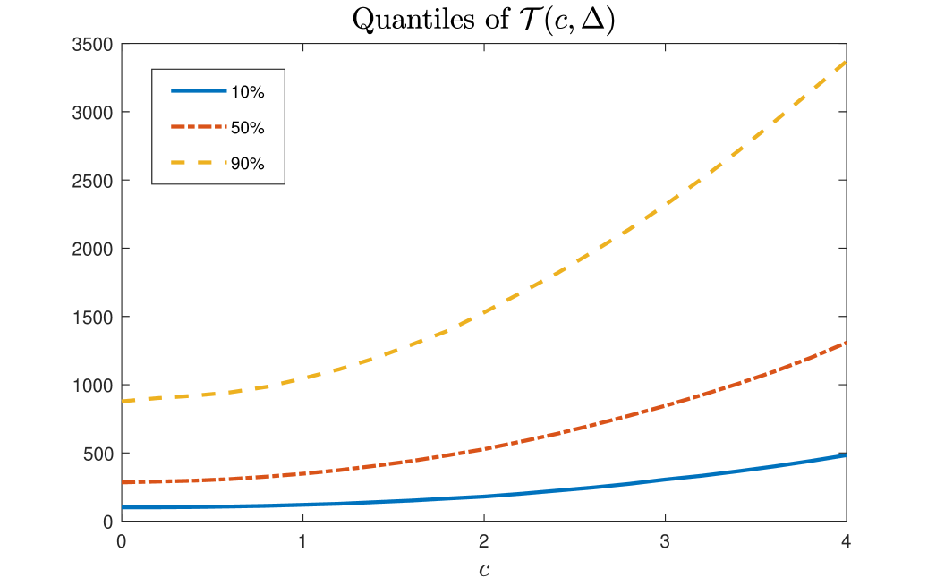
The above theorem implies that the asymptotic power of Tn(s)T_{n}^{(s)} and TnT_{n} depends on the joint behavior of δ\delta and ΣF\|\Sigma\|_{F}, holding nn as fixed. If Σ\Sigma is the identity matrix, then Tn(s)T_{n}^{(s)} and TnT_{n} will exhibit different power behaviors according to whether δ/p1/4\|\delta\|/p^{1/4} converges to zero, infinity, or some constant cn(0,)c_{n}\in(0,\infty). In addition, under the local alternative, the limiting distribution of Tn(s)T_{n}^{(s)} and TnT_{n} under the sequantial asymptotics coincides with that in Wang et al., (2022) under the joint asymptotics, see Theorem 3.5 therein. In Figure 1, we plot 𝒯(c,Δ)\mathcal{T}(c,\Delta) at 10%, 50% and 90% quantile levels with bb^{*} fixed at 1/21/2 and it suggests that 𝒯(c,Δ)\mathcal{T}(c,\Delta) is stochastically increasing with cc, which further supports the consistency of both tests.

Refer to caption
Figure 1: 𝒯(c,Δ)\mathcal{T}(c,\Delta) at 10%, 50% and 90% quantile levels.

3.4 Analysis Under Stronger Dependence Structure

In this section, we focus on a special class of probability models for high dimensional data termed “randomly scaled ρ\rho-mixing (RSRM)” sequence.

Definition 3.2 (RSRM, Chakraborty and Chaudhuri, (2017)).

A sequence (η1,η2,)(\eta_{1},\eta_{2},\cdots) is a randomly scaled ρ\rho-mixing sequence if there exist a zero mean ρ\rho-mixing squence (ξ1,ξ2,)(\xi_{1},\xi_{2},\cdots) and an independent positive non-degenerate random variable RR such that ηi=ξi/R\eta_{i}=\xi_{i}/R, i=1,2,i=1,2,\cdots.

RSRM sequences introduce stronger dependence structure among the coordinates than ρ\rho-mixing sequences, and many models fall into this category, see, e.g. elliptically symmetric models in Wang et al., (2015) and non-Gaussian sequences in Cai et al., (2014).

Assumption 3.5.

Suppose Yi=Xi/Ri+μiY_{i}=X_{i}/R_{i}+\mu_{i}, where {Xi}i=1n\{X_{i}\}_{i=1}^{n} satisfies Assumptions 3.1 and 3.2, and {Ri}i=1n\{R_{i}\}_{i=1}^{n} are i.i.d. copies of a positive random variable RR.

Clearly, when RR is degenerate (i.e., a positive constant), Assumption 3.5 reduces to the model assumed in previous sections. However, when RR is non-degenerate, Assumption 3.5 imposes stronger dependence structure on coordinates of YiY_{i} than ρ\rho-mixing sequences, and hence result in additional theoretical difficulties. We refer to Chakraborty and Chaudhuri, (2017) for more discussions of RSRM sequences.

Theorem 3.4.

Suppose Assumption 3.5 holds, then under H0H_{0},

(i) let n={Ri}i=1n,\mathcal{R}_{n}=\{R_{i}\}_{i=1}^{n}, for any fixed n8n\geq 8, if 𝔼(Ri2)<\mathbb{E}(R_{i}^{2})<\infty and 𝔼(Ri2)<\mathbb{E}(R_{i}^{-2})<\infty, as pp\to\infty, there exists two random variables 𝒯n(n,s)\mathcal{T}_{n}^{(\mathcal{R}_{n},s)} and 𝒯n(n)\mathcal{T}_{n}^{(\mathcal{R}_{n})} dependent on n\mathcal{R}_{n} such that,

Tn(s)𝒟𝒯n(n,s),Tn𝒟𝒯n(n).T_{n}^{(s)}\overset{\mathcal{D}}{\rightarrow}\mathcal{T}_{n}^{(\mathcal{R}_{n},s)},\quad T_{n}\overset{\mathcal{D}}{\rightarrow}\mathcal{T}_{n}^{(\mathcal{R}_{n})}.

(ii) Furthermore, if we further assume 𝔼(Ri4)<\mathbb{E}(R_{i}^{4})<\infty and 𝔼(Ri4)<\mathbb{E}(R_{i}^{-4})<\infty, then as nn\to\infty, we have

𝒯n(n,s)𝒟𝒯,𝒯n(n)𝒟𝒯,\mathcal{T}_{n}^{(\mathcal{R}_{n},s)}\overset{\mathcal{D}}{\rightarrow}\mathcal{T},\quad\mathcal{T}_{n}^{(\mathcal{R}_{n})}\overset{\mathcal{D}}{\rightarrow}\mathcal{T},

where 𝒯\mathcal{T} is defined in (6).

In general, if the sample size nn is small and YiY_{i} is generated from an RSRM sequence, the unconditional limiting distributions of Tn(s)T_{n}^{(s)} and TnT_{n} as pp\to\infty are no longer pivotal due to the randomness in RiR_{i}. Nevertheless, using the pivotal limiting distribution 𝒯n\mathcal{T}_{n} in hypothesis testing can still deliver relatively good performance for Tn(s)T_{n}^{(s)} in both size and power, see Section 5.1 below for numerical evidence. If nn is also diverging, the same pivotal limiting distribution as presented in Theorem 3.1 (ii) and in Theorem 3.4 of Wang et al., (2022) can still be reached.

Let ΣY\Sigma_{Y} be the covariance of YiY_{i} (or equivalently Xi/RiX_{i}/R_{i}), the next theorem provides with the asymptotic behavior under local alternative for the RSRM model.

Theorem 3.5.

Suppose Assumptions 3.4 and 3.5 hold, then under the local alternative such that nΣYF1δ2cn(0,)n\|\Sigma_{Y}\|_{F}^{-1}\|\delta\|^{2}\to c_{n}\in(0,\infty),

(i) let n={Ri}i=1n,\mathcal{R}_{n}=\{R_{i}\}_{i=1}^{n}, for any fixed n8n\geq 8, if 𝔼(Ri2)<\mathbb{E}(R_{i}^{2})<\infty and 𝔼(Ri2)<\mathbb{E}(R_{i}^{-2})<\infty, as pp\to\infty, there exists two random variables 𝒯n(n,s)(Δn(n,s))\mathcal{T}_{n}^{(\mathcal{R}_{n},s)}(\Delta_{n}^{(\mathcal{R}_{n},s)}) and 𝒯n(n)(Δn)\mathcal{T}_{n}^{(\mathcal{R}_{n})}(\Delta_{n}) dependent on n\mathcal{R}_{n} such that,

Tn(s)𝒟𝒯n(n,s)(cn,Δn(n,s)),Tn𝒟𝒯n(n)(cn,Δn).T_{n}^{(s)}\overset{\mathcal{D}}{\rightarrow}\mathcal{T}_{n}^{(\mathcal{R}_{n},s)}(c_{n},\Delta_{n}^{(\mathcal{R}_{n},s)}),\quad T_{n}\overset{\mathcal{D}}{\rightarrow}\mathcal{T}_{n}^{(\mathcal{R}_{n})}(c_{n},\Delta_{n}).

(ii) Furthermore, if we assume 𝔼(Ri4)<\mathbb{E}(R_{i}^{4})<\infty and 𝔼(Ri4)<\mathbb{E}(R_{i}^{-4})<\infty, and limncn=c(0,)\lim_{n\to\infty}c_{n}=c\in(0,\infty), then as nn\to\infty, we have

𝒯n(n,s)(cn,Δn(n,s))𝒟𝒯(Kc,Δ),𝒯n(n)(cn,Δn(n))𝒟𝒯(c,Δ),\mathcal{T}_{n}^{(\mathcal{R}_{n},s)}(c_{n},\Delta_{n}^{(\mathcal{R}_{n},s)})\overset{\mathcal{D}}{\rightarrow}\mathcal{T}(Kc,\Delta),\quad\mathcal{T}_{n}^{(\mathcal{R}_{n})}(c_{n},\Delta_{n}^{(\mathcal{R}_{n})})\overset{\mathcal{D}}{\rightarrow}\mathcal{T}(c,\Delta),

where 𝒯(c,Δ)\mathcal{T}(c,\Delta) is defined in (7), and

K=𝔼1[R1R2(R12+R32)(R22+R32)]𝔼(R12)𝔼2[R1R2R12+R22]>1K=\mathbb{E}^{-1}\Big{[}\frac{R_{1}R_{2}}{\sqrt{(R_{1}^{2}+R_{3}^{2})(R_{2}^{2}+R_{3}^{2})}}\Big{]}\mathbb{E}(R_{1}^{-2})\mathbb{E}^{2}\Big{[}\frac{R_{1}R_{2}}{\sqrt{R_{1}^{2}+R_{2}^{2}}}\Big{]}>1

is a constant.

For the RSRM model, similar to Theorem 3.4 (i), the fixed-nn limiting distributions of Tn(s)T_{n}^{(s)} and TnT_{n} are non-pivotal under local alternatives. However, the distribution of Tn(s)T_{n}^{(s)} under sequential limit is pivotal 𝒯(Kc,Δ)\mathcal{T}(Kc,\Delta) while that of TnT_{n} is 𝒯(c,Δ)\mathcal{T}(c,\Delta). The multiplicative constant K>1K>1 suggests that for the RSRM model, using Tn(s)T_{n}^{(s)} could be more powerful as 𝒯(c,Δ)\mathcal{T}(c,\Delta) is expected to be monotone in cc, see Figure 1 above. This finding coincides with Chakraborty and Chaudhuri, (2017) where they showed that using spatial sign based U-statistics for testing the equality of two high dimensional means could be more powerful than the conventional mean-based ones in Chen and Qin, (2010). Thus, when strong coordinate-wise dependence is exhibited in the data, Tn(s)T_{n}^{(s)} is more preferable.

4 Multiple Change-point Estimation

In real applications, in addition to change-point testing, another important task is to estimate the number and locations of these change-points. In this section, we assume there are m1m\geq 1 change-points and are denoted by 𝒌=(k1,k2,,km){1,2,,n}{\bm{k}}=(k_{1},k_{2},\cdots,k_{m})\subset\{1,2,\cdots,n\}. A commonly used algorithm for many practitioners would be binary segmentation (BS), where the data segments are recursively split at the maximal points of the test statistics until the null of no change-points is not rejected for each segment. However, as criticized by many researchers, BS tends to miss potential change-points when non-monotonic change patterns are exhibited. Hence, many algorithms have been proposed to overcome this drawback. Among them, wild binary segmentation (WBS) by Fryzlewicz, (2014) and its variants have become increasingly popular because of their easy-to-implement procedures. The main idea of WBS is to perform BS on randomly generated sub-intervals so that some sub-intervals can localize at most one change-point (with high probability). As pointed out by Kovács et al., (2020), WBS relies on randomly generated sub-intervals and different researchers may obtain different estimates. Hence, Kovács et al., (2020) propose seeded binary segmentation (SBS) algorithm based on deterministic construction of these sub-intervals with relatively cheaper computational costs so that results are replicable. To this end, we combine the spatial signed SN test with SBS to achieve the task of multiple change-point estimation, and we call it SBS-SN(s). We first introduce the concept of seeded sub-intervals.

Definition 4.1 (Seeded Sub-Intervals, Kovács et al., (2020)).

Let α[1/2,1)\alpha\in[1/2,1) denote a given decay parameter. For 1klog1/α(n)1\leq k\leq\lfloor\log_{1/\alpha}(n)\rfloor (i.e. logarithm with base 1/α1/\alpha) define the kk-th layer as the collection of nkn_{k} intervals of initial length lkl_{k} that are evenly shifted by the deterministic shift sks_{k} as follows:

k=i=1nk{((i1)sk,(i1)sk+lk)}\mathcal{I}_{k}=\bigcup_{i=1}^{n_{k}}\left\{\left(\left\lfloor(i-1)s_{k}\right\rfloor,\left\lceil(i-1)s_{k}+l_{k}\right\rceil\right)\right\}

where nk=2(1/α)k11,lk=10nαk1/10n_{k}=2\left\lceil(1/\alpha)^{k-1}\right\rceil-1,l_{k}=10\lceil n\alpha^{k-1}/10\rceil and sk=(nlk)/(nk1).s_{k}=\left(n-l_{k}\right)/\left(n_{k}-1\right). The overall collection of seeded intervals is

α(n)=k=1log1/α(n)k.\mathcal{I}_{\alpha}(n)=\bigcup_{k=1}^{\left\lceil\log_{1/\alpha}(n)\right\rceil}\mathcal{I}_{k}.

Let α[1/2,1)\alpha\in[1/2,1) be a decay parameter, denote α(n)\mathcal{I}_{\alpha}(n) as the set of seeded intervals based on Definition 4.1. For each sub-interval (a,b)α(n)(a,b)\in\mathcal{I}_{\alpha}(n), we calculate the spatial signed SN test

T(s)(a,b)=maxk{a+3,,b4}(D(s)(k;a,b))2Wba+1(s)(k;a,b),ba7,T^{(s)}(a,b)=\max_{k\in\{a+3,\cdots,b-4\}}\frac{(D^{(s)}(k;a,b))^{2}}{W_{b-a+1}^{(s)}(k;a,b)},\quad b-a\geq 7,

where D(s)(k;a,b))D^{(s)}(k;a,b)) and Wba+1(s)(k;a,b)W_{b-a+1}^{(s)}(k;a,b) are defined in (3) and (4). We obtain the p-value of the sub-interval test statistic T(s)(a,b)T^{(s)}(a,b) based on the fixed-nn asymptotic distribution 𝒯ba+1\mathcal{T}_{b-a+1}. SBS-SN(s) then finds the smallest p-value evaluated at all sub-intervals and compare it with a predetermined threshold level ζp\zeta_{p}. If the smallest p-value is also smaller than ζp\zeta_{p}, denote the corresponding sub-interval where the smallest p-value is achived as (a,b)(a^{*},b^{*}) and estimate the change-point by k^=argmaxk{a+3,,b4}(D(s)(k;a,b))2Wba+1(s)(k;a,b)\hat{k}=\arg\max_{k\in\{a^{*}+3,\cdots,b^{*}-4\}}\frac{(D^{(s)}(k;a^{*},b^{*}))^{2}}{W_{b^{*}-a^{*}+1}^{(s)}(k;a^{*},b^{*})}. Once a change-point is identified, SBS-SN(s) then divides the data sample into two subsamples accordingly and apply the same procedure to each of them. The process is implemented recursively until no change-point is detected. Details are provided in Algorithm 1.

Input: Data {Yt}t=1n\{Y_{t}\}_{t=1}^{n}, threshold p-value ζp(0,1)\zeta_{p}\in(0,1), SBS intervals α(n)\mathcal{I}_{\alpha}(n).
Output: Estimated number of change-points m^\widehat{m} and estimated change-points set 𝒌^\hat{\bm{k}}
Initialization: SBS-SN(s) (1,n,ζp)(1,n,\zeta_{p})
Procedure: SBS-SN(s) (a,b,ζp)(a,b,\zeta_{p})
1 if ba+1<8b-a+1<8 then
2  Stop
3else
4 (a,b):={i:[ai,bi]α(n),[ai,bi][a,b],biai+18}\mathcal{M}_{(a,b)}:=\{i:[a_{i},b_{i}]\in\mathcal{I}_{\alpha}(n),[a_{i},b_{i}]\subset[a,b],b_{i}-a_{i}+1\geq 8\} ;
5   for each i(a,b)i\in\mathcal{M}_{(a,b)}, find the p-value pip_{i} of T(s)(ai,bi)T^{(s)}(a_{i},b_{i}) based on 𝒯biai+1\mathcal{T}_{b_{i}-a_{i}+1};
6 i=argmini(a,b)pii^{*}=\arg\min_{i\in\mathcal{M}_{(a,b)}}p_{i};
7 if pi<ζpp_{i^{*}}<\zeta_{p} then
8    k=argmaxk{ai+3,,bi4}(D(s)(k;ai,bi))2Wbiai+1(s)(k;ai,bi)k^{*}=\arg\max_{k\in\{a_{i^{*}}+3,\cdots,b_{i^{*}}-4\}}\frac{(D^{(s)}(k;a_{i^{*}},b_{i^{*}}))^{2}}{W_{b_{i^{*}}-a_{i^{*}}+1}^{(s)}(k;a_{i^{*}},b_{i^{*}})} ;
9    𝒌^=𝒌^k\widehat{\bm{k}}=\widehat{\bm{k}}\cup k^{*}, m^=m^+1\widehat{m}=\widehat{m}+1;
10      SBS-SN(s) (a,k,ζp)(a,k^{*},\zeta_{p});
11      SBS-SN(s) (k+1,b,ζp)(k^{*}+1,b,\zeta_{p});
12    
13 else
14     Stop
15   end if
16 
17 end if
Algorithm 1 SBS-SN(s)

Our SBS-SN(s) algorithm differs from WBS-SN algorithm in Wang et al., (2022) and Zhang et al., (2021) in two aspects. First, WBS-SN is built on WBS, which relies on randomly generated intervals while SBS relies on deterministic intervals. As documented in Kovács et al., (2020), WBS is computationally more demanding than SBS. Second, the threshold used in WBS-SN is universal for each sub-interval, depends on the sample size nn and dimension pp and needs to be simulated via extensive Monte Carlo simulations. Generally speaking, WBS-SN requires simulating a new threshold each time for a new dataset. By contrast, our estimation procedure is based on p-values under the fixed-nn asymptotics, which takes into account the interval length ba+1b-a+1 for each sub-interval (a,b)(a,b). When implementing either WBS or SBS, inevitably, there will be intervals of small lengths. Hence, the universal threshold may not be suitable as it does not take into account the effect of different interval lengths. In order to alleviate the problem of multiple testing, we may set a small threshold number for ζp\zeta_{p}, such as 0.0001 or 0.0005. Furthermore, the WBS-SN requires to specify a minimal interval lentgh which can affect the finite sample performance. In this work, when generating seed sub-intervals as in Definition 4.1, the lengths of these intervals are set as integer values times 10 to reduce the computational cost for simulating fixed-nn asymptotic distribution 𝒯n\mathcal{T}_{n}. Therefore, we only require the knowledge of {𝒯n}n=10,20,\{\mathcal{T}_{n}\}_{n=10,20,\cdots} for SBS-SN(s) to work, which can be simulated once for good and do not change with a new dataset.

5 Numerical Experiments

This section examines the finite sample behavior of the proposed tests and multiple change-point estimation algorithm SBS-SN(s) via simulation studies.

5.1 Size and Power

We first assess the performance of Tn(s)T_{n}^{(s)} with respect to various covariance structure of the data. Consider the following data generating process with p=100p=100 and n{10,20,50,100,200}n\in\{10,20,50,100,200\}:

Yi=δ𝟏(i>0.5n)+Xi,Y_{i}=\delta\mathbf{1}(i>0.5n)+X_{i},

where δ\delta represents the mean shift vector, and {Xi}i=1n\{X_{i}\}_{i=1}^{n} are i.i.d copies of XX based on the following specifications:

  1. (i)

    X𝒩(𝟎,Ip)X\sim\mathcal{N}(\mathbf{0},I_{p});

  2. (ii)

    Xt5(Ip)X\sim t_{5}(I_{p});

  3. (iii)

    Xt3(Ip)X\sim t_{3}(I_{p});

  4. (iv)

    X=(X(1),,X(p))X=(X^{(1)},\cdots,X^{(p)})^{\prime}, X(t)=ρX(t1)+ϵtX^{(t)}=\rho X^{(t-1)}+\epsilon_{t}, t=1,,pt=1,\cdots,p, where ϵt𝒩(0,1)/2\epsilon_{t}\sim\mathcal{N}(0,1)/2 are i.i.d random variables;

  5. (v)

    X=(X(1),,X(p))X=(X^{(1)},\cdots,X^{(p)})^{\prime}, X(t)=ρX(t1)+ϵtX^{(t)}=\rho X^{(t-1)}+\epsilon_{t}, t=1,,pt=1,\cdots,p, where ϵtt5/2\epsilon_{t}\sim t_{5}/2 are i.i.d random variables;

  6. (vi)

    X=R/UX=R/U, R=(R(1),,R(p))R=(R^{(1)},\cdots,R^{(p)})^{\prime}, R(t)=ρR(t1)+ϵtR^{(t)}=\rho R^{(t-1)}+\epsilon_{t}, t=1,,pt=1,\cdots,p, where ϵt𝒩(0,1)/2\epsilon_{t}\sim\mathcal{N}(0,1)/2 are i.i.d random variables, and UExp(1)U\sim\text{Exp}(1) is independently generated;

  7. (vii)

    X=R/UX=R/U, R=(R(1),,R(p))R=(R^{(1)},\cdots,R^{(p)})^{\prime}, R(t)=ρR(t1)+ϵtR^{(t)}=\rho R^{(t-1)}+\epsilon_{t}, t=1,,pt=1,\cdots,p, where ϵtt5/2\epsilon_{t}\sim t_{5}/2 are i.i.d random variables, and UExp(1)U\sim\text{Exp}(1) is independently generated;

where tν(Ip)t_{\nu}(I_{p}) is the multivariate tt distribution with degree of freedom ν\nu and covariance IpI_{p}; Exp(1)\text{Exp}(1) is the exponential distribution with mean 11.

Case (i) assumes that coordinates of XX are independent and light-tailed; Cases (ii) and (iii) consider the scenario of heavy-tailedness of XX; Cases (iv) and (v) assume the coordinates of XX are consecutive random observations from a stationary AR(1) model with autoregressive coefficient ρ=0.7\rho=0.7; and Cases (vi) and (vii) assume the coordinates of XX are generated from an RSRM with ρ=0.7\rho=0.7.

Table 2 shows the empirical rejection rate of TnT_{n} and Tn(s)T_{n}^{(s)} in percentage based on 1000 replications under the null with H0:H_{0}: δ=𝟎\delta=\mathbf{0}; dense alternative Ha1:δ=1/p𝟏pH_{a}^{1}:\delta=1/\sqrt{p}\mathbf{1}_{p}; and sparse alternative Ha2:δ=(𝟏2,𝟎p2)H_{a}^{2}:\delta=(\mathbf{1}_{2}^{\top},\mathbf{0}_{p-2}^{\top})^{\top}. We compare the approximation using the limiting null distribution of fixed-nn asymptotics 𝒯n\mathcal{T}_{n} and sequential asymptotics 𝒯\mathcal{T} at 5%5\% level.

Table 2: Size and power comparison of TnT_{n} and Tn(s)T_{n}^{(s)}
H0H_{0} Ha1H_{a}^{1} Ha2H_{a}^{2}
Case Test Limit nn 10 20 50 100 200 10 20 50 100 200 10 20 50 100 200
(i) TnT_{n} 𝒯n\mathcal{T}_{n} 5.6 4.8 6.9 4.0 6.4 6.3 6.5 15.2 34.7 77.1 7.3 11.0 34.1 78.0 99.9
𝒯\mathcal{T} 27.4 9.0 7.4 4.1 6.7 29.9 11.2 16.5 35.2 77.8 33.7 18.1 34.9 78.1 99.9
Tn(s)T_{n}^{(s)} 𝒯n\mathcal{T}_{n} 5.5 4.8 6.2 4.3 6.6 6.2 5.9 15.0 33.4 76.7 7.2 10.4 33.3 77.7 99.8
𝒯\mathcal{T} 28.5 8.7 6.8 4.4 7.1 29.8 10.8 15.7 34.6 77.6 33.5 17.3 34.6 78.6 99.8
(ii) TnT_{n} 𝒯n\mathcal{T}_{n} 6.9 6.4 6.8 4.3 6.0 7.2 7.2 11.7 18.5 41.4 8.0 8.8 22.0 47.2 87.3
𝒯\mathcal{T} 31.8 12.6 7.6 4.3 6.2 31.8 12.4 12.8 19.0 42.5 33.9 15.3 22.9 47.5 87.4
Tn(s)T_{n}^{(s)} 𝒯n\mathcal{T}_{n} 5.3 5.3 6.2 4.1 5.6 5.7 5.5 11.8 26.1 59.6 6.4 8.1 26.7 62.9 96.8
𝒯\mathcal{T} 28.2 9.7 6.7 4.2 5.7 28.5 10.0 12.6 27.0 60.4 30.8 14.4 28.0 63.2 96.8
(iii) TnT_{n} 𝒯n\mathcal{T}_{n} 9.0 9.5 9.2 6.7 7.9 10.0 10.4 11.8 14.2 25.7 9.8 12.3 17.9 27.9 57.5
𝒯\mathcal{T} 35.8 16.1 9.6 6.9 8.5 35.6 16.1 12.6 14.7 26.0 36.8 18.7 18.8 28.7 58.2
Tn(s)T_{n}^{(s)} 𝒯n\mathcal{T}_{n} 5.6 5.0 6.4 4.8 6.4 5.7 4.9 10.5 21.2 50.2 6.2 6.9 21.9 53.0 93.4
𝒯\mathcal{T} 27.5 9.6 7.0 4.9 6.8 29.2 9.3 11.4 21.7 50.8 28.6 12.8 23.0 53.9 93.7
(iv) TnT_{n} 𝒯n\mathcal{T}_{n} 5.9 4.8 6.1 6.8 5.4 6.5 8.6 23.5 46.4 78.8 9.3 14.7 43.2 83.8 99.6
𝒯\mathcal{T} 28.1 9.2 6.7 6.9 5.7 30.9 13.8 24.6 47.4 79.1 33.9 20.1 44.4 84.0 99.6
Tn(s)T_{n}^{(s)} 𝒯n\mathcal{T}_{n} 4.8 3.9 6.0 6.3 5.4 5.5 7.1 22.5 44.2 77.9 6.9 13.0 41.5 84.1 99.8
𝒯\mathcal{T} 27.6 8.2 6.5 6.6 5.4 30.6 12.2 23.5 45.3 78.1 33.1 18.8 43.0 84.6 99.8
(v) TnT_{n} 𝒯n\mathcal{T}_{n} 7.0 7.6 6.0 6.8 6.1 8.6 11.1 17.5 30.1 54.2 9.4 11.3 26.7 56.7 94.0
𝒯\mathcal{T} 33.5 12.9 6.6 7.2 6.1 33.6 16.9 17.9 30.4 54.6 34.4 18.3 27.9 57.1 94.2
Tn(s)T_{n}^{(s)} 𝒯n\mathcal{T}_{n} 5.3 4.4 5.0 6.9 5.2 6.1 7.5 18.5 37.1 65.2 5.6 9.4 35.2 73.7 98.7
𝒯\mathcal{T} 29.3 8.5 5.3 7.5 5.5 30.5 11.8 19.0 37.7 65.6 30.6 14.1 35.8 74.2 98.8
(vi) TnT_{n} 𝒯n\mathcal{T}_{n} 34.7 39.7 39.2 34.6 33.6 34.6 40.7 39.4 35.6 34.2 35.0 39.6 40.1 34.3 33.8
𝒯\mathcal{T} 60.2 46.7 40.5 34.9 34.1 62.5 47.5 40.3 36.1 34.8 60.6 46.9 41.0 34.4 34.1
Tn(s)T_{n}^{(s)} 𝒯n\mathcal{T}_{n} 5.0 4.2 5.3 5.9 5.9 6.0 4.8 11.3 20.1 35.3 5.6 7.1 16.8 37.2 73.5
𝒯\mathcal{T} 27.9 8.6 5.7 6.2 6.1 28.1 10.0 12.0 20.3 35.4 28.2 11.9 17.6 38.0 74.0
(vii) TnT_{n} 𝒯n\mathcal{T}_{n} 33.7 40.6 37.9 36.5 36.6 34.3 40.3 37.9 37.0 36.9 33.5 40.6 38.3 36.9 36.8
𝒯\mathcal{T} 61.9 47.3 38.6 37.2 36.8 62.2 46.5 39.1 37.4 37.1 61.5 47.7 39.8 37.7 36.9
Tn(s)T_{n}^{(s)} 𝒯n\mathcal{T}_{n} 4.3 4.4 5.2 6.4 6.0 5.1 6.2 9.5 17.5 32.9 5.1 5.8 14.1 28.5 62.5
𝒯\mathcal{T} 30.2 8.4 5.5 6.7 6.5 30.6 10.1 10.2 17.7 33.5 30.4 9.2 15.3 29.1 63.0

We summarize the findings of Table 2 as follows: (1) both TnT_{n} and Tn(s)T_{n}^{(s)} suffer from severe size distortion using sequential asymptotics 𝒯\mathcal{T} if nn is small (i.e., n=10,20,50n=10,20,50); (2) both fixed-nn asymptotics 𝒯n\mathcal{T}_{n} and large-nn asymptotics 𝒯\mathcal{T} work well for TnT_{n} and Tn(s)T_{n}^{(s)} when nn is large under weak dependence in coordinates (cases (i)-(v)); (3) TnT_{n} and Tn(s)T_{n}^{(s)} are both accurate in size and comparable in power performance when XiX_{i}’s are light-tailed (cases (i),(ii), (iv) and (v)) if appropriate limiting distributions are used; (4) TnT_{n} is slightly oversized compared with Tn(s)T_{n}^{(s)} under heavy-tailed distributions (case (iii)); (5) when strong dependence is exhibited in coordinates (cases (vi) and (vii)), (Tn(s),𝒯n)(T_{n}^{(s)},\mathcal{T}_{n}) still works for small nn while other combinations of tests and asymptotics generally fail; (6) increasing the data length nn enhances power under all settings while increasing dependence in coordinates generally reduces power. Overall, the spatial signed SN test using fixed-nn asymptotic critical value outperforms all other tests and should be preferred due to its robustness and size accuracy.

5.2 Segmentation

We then examine the numerical performance of SBS-SN(s) by considering the multiple change-points models in Wang et al., (2022). For p=50p=50 and n=120n=120, we generate i.i.d. samples of {Xi}i=1n\{X_{i}\}_{i=1}^{n}, where XiX_{i}’s are either normally distributed, i.e., case (i); or RSRM sequences, i.e., case (vii) with autoregressive coefficient ρ=0.3.\rho=0.3. We assume there are three change points at k=k= 30, 60 and 90. Denote the changes in mean by 𝜽1\bm{\theta}_{1}, 𝜽2\bm{\theta}_{2} and 𝜽3\bm{\theta}_{3}, where 𝜽1=𝜽2=𝜽3=h/d(𝟏d,𝟎pd)\bm{\theta}_{1}=-\bm{\theta}_{2}=\bm{\theta}_{3}=\sqrt{h/d}(\bm{1}_{d}^{\top},\bm{0}_{p-d}^{\top})^{\top}, d{5,p}d\in\{5,p\} and h{2.5,4}.h\in\{2.5,4\}. Here, dd represents the sparse or dense alternatives while hh represents the signal strength. For example, we refer to the choice of d=5d=5 and h=2.5h=2.5 as Sparse(2.5) and d=pd=p, h=4h=4 as Dense(4).

To assess the estimation accuracy, we consider (1) the differences between the estimated number of change-points m^\hat{m} and the truth m=3m=3; (2) Mean Squared Error (MSE) between m^\hat{m} and the truth m=3m=3; (3) the adjusted Rand index (ARI) which measures the similarity between two partitions of the same observations. Generally speaking, a higher ARI (with the maximum value of 1) indicates more accurate change-point estimation, see Hubert and Arabie, (1985) for more details.

We also report the estimation results using WBS-SN in Wang et al., (2022) and SBS-SN (by replacing WBS with SBS in Wang et al., (2022)). The superiority of WBS-SN over other competing methods can be found in Wang et al., (2022) under similar simulation settings. For SBS based estimation results, we vary the decay rate α{21/2,21/4}\alpha\in\{2^{-1/2},2^{-1/4}\}, which are denoted by SBS1 and SBS2 respectively. Here, the thresholds in above algorithms are either Monte Carlo simulated constant ζn\zeta_{n} for all sub-interval test statistics; or prespecified quantile level ζp(0,1)\zeta_{p}\in(0,1) based on p-values reported by these sub-interval statistics. Here, we fix ζn\zeta_{n} as the 95% quantile levels of the maximal test statistics based on 5000 simulated Gaussian data with no change-points as in Wang et al., (2022) while ζp\zeta_{p} is set as 0.001 (the results using 0.005 is similar hence omitted). We replicate all experiments 500 times, and results for dense changes and sparse changes are reported in Table 3 and Table 4, respectively.

From Table 3, we find that (1) WBS-SN and SBS-SN tend to produce close estimation accuracy holding the form of XX and signal strength fixed; (2) different decay rates have some impact on the performance of SBS-SN methods, and when the signal is weak the impact is noticeable; (3) increasing the signal strength of change-points boosts the detection power for all methods; (4) using ζp\zeta_{p} gives more accurate estimation than using ζn\zeta_{n} in SBS-SN when data is normally distributed with weak signal level and they work comparably in other settings; (5) when XX is normally distributed, SBS-SN(s) works comparably with other estimation algorithms while for RSRM sequences, our SBS-SN(s) greatly outperforms other methods. The results in Table 4 are similar. These findings together suggest substantial gain in detection performance using SBS-SN(s) due to its robustness to heavy-tailedness and stronger dependence in the coordinates.

Table 3: Estimation results with dense changes.
Test Threshold XX m^m\hat{m}-m MSE ARI
<-1 -1 0 1 >1
Dense(2.5) WBS TnT_{n} ζn\zeta_{n} Normal 95 156 246 3 0 1.278 0.729
SBS1 TnT_{n} ζn\zeta_{n} Normal 76 206 214 4 0 1.068 0.742
SBS2 TnT_{n} ζn\zeta_{n} Normal 32 195 266 7 0 0.660 0.809
SBS1 TnT_{n} ζp\zeta_{p} Normal 0 0 𝟒𝟔𝟒\bm{464} 35 1 0.078 0.929\bm{0.929}
SBS2 TnT_{n} ζp\zeta_{p} Normal 0 10 𝟒𝟔𝟔\bm{466} 23 1 0.074\bm{0.074} 0.931\bm{0.931}
SBS1 Tn(s)T_{n}^{(s)} ζp\zeta_{p} Normal 0 1 𝟒𝟔𝟗\bm{469} 29 1 0.068\bm{0.068} 0.928\bm{0.928}
SBS2 Tn(s)T_{n}^{(s)} ζp\zeta_{p} Normal 0 19 463 18 0 0.074\bm{0.074} 0.926
WBS TnT_{n} ζn\zeta_{n} RSRM 64 89 133 104 110 2.668 0.461
SBS1 TnT_{n} ζn\zeta_{n} RSRM 35 58 116 107 184 3.612 0.462
SBS2 TnT_{n} ζn\zeta_{n} RSRM 38 72 114 130 146 3.032 0.470
SBS1 TnT_{n} ζp\zeta_{p} RSRM 8 6 32 84 376 8.792 0.653
SBS2 TnT_{n} ζp\zeta_{p} RSRM 57 43 104 106 233 4.508 0.532
SBS1 Tn(s)T_{n}^{(s)} ζp\zeta_{p} RSRM 3 65 412 20 0 0.194 0.880
SBS2 Tn(s)T_{n}^{(s)} ζp\zeta_{p} RSRM 11 121 355 13 0 0.356 0.850
Dense(4) WBS TnT_{n} ζn\zeta_{n} Normal 0 7 486 7 0 0.028 0.948
SBS1 TnT_{n} ζn\zeta_{n} Normal 0 21 467 12 0 0.066 0.936
SBS2 TnT_{n} ζn\zeta_{n} Normal 0 23 464 13 0 0.072 0.945
SBS1 TnT_{n} ζp\zeta_{p} Normal 0 0 464 34 2 0.084 0.937
SBS2 TnT_{n} ζp\zeta_{p} Normal 0 0 476 23 1 0.054 0.943
SBS1 Tn(s)T_{n}^{(s)} ζp\zeta_{p} Normal 0 0 468 31 1 0.070 0.936
SBS2 Tn(s)T_{n}^{(s)} ζp\zeta_{p} Normal 0 0 482 18 0 0.036 0.942
WBS TnT_{n} ζn\zeta_{n} RSRM 64 89 133 104 110 2.668 0.461
SBS1 TnT_{n} ζn\zeta_{n} RSRM 26 67 107 115 185 3.732 0.484
SBS2 TnT_{n} ζn\zeta_{n} RSRM 33 74 115 125 153 3.146 0.489
SBS1 TnT_{n} ζp\zeta_{p} RSRM 27 25 71 93 309 6.604 0.579
SBS2 TnT_{n} ζp\zeta_{p} RSRM 39 33 103 114 244 4.740 0.559
SBS1 Tn(s)T_{n}^{(s)} ζp\zeta_{p} RSRM 0 10 469 20 1 0.068 0.918
SBS2 Tn(s)T_{n}^{(s)} ζp\zeta_{p} RSRM 0 35 451 14 0 0.098 0.911

Note: Top 3 methods are in bold format.

Table 4: Estimation results with sparse changes.
Test Threshold XX m^m\hat{m}-m MSE ARI
<-1 -1 0 1 >1
Sparse(2.5) WBS TnT_{n} ζn\zeta_{n} Normal 78 147 274 1 0 1.050 0.759
SBS1 TnT_{n} ζn\zeta_{n} Normal 59 214 223 4 0 0.928 0.760
SBS2 TnT_{n} ζn\zeta_{n} Normal 20 185 287 8 0 0.546 0.829
SBS1 TnT_{n} ζp\zeta_{p} Normal 0 1 464 34 1 0.078 0.929
SBS2 TnT_{n} ζp\zeta_{p} Normal 0 13 465 21 1 0.076 0.930
SBS1 Tn(s)T_{n}^{(s)} ζp\zeta_{p} Normal 0 2 470 27 1 0.066 0.927
SBS2 Tn(s)T_{n}^{(s)} ζp\zeta_{p} Normal 0 23 460 17 0 0.080 0.924
WBS TnT_{n} ζn\zeta_{n} RSRM 70 97 121 102 110 2.682 0.449
SBS1 TnT_{n} ζn\zeta_{n} RSRM 38 51 110 124 177 3.572 0.460
SBS2 TnT_{n} ζn\zeta_{n} RSRM 39 66 122 122 151 3.100 0.474
SBS1 TnT_{n} ζp\zeta_{p} RSRM 38 35 75 109 278 5.800 0.447
SBS2 TnT_{n} ζp\zeta_{p} RSRM 84 69 129 108 179 3.258 0.528
SBS1 Tn(s)T_{n}^{(s)} ζp\zeta_{p} RSRM 5 64 414 17 0 0.212 0.872
SBS2 Tn(s)T_{n}^{(s)} ζp\zeta_{p} RSRM 8 117 364 11 0 0.330 0.851
Sparse(4) WBS TnT_{n} ζn\zeta_{n} Normal 0 7 486 7 0 0.028 0.958
SBS1 TnT_{n} ζn\zeta_{n} Normal 0 19 468 13 0 0.064 0.938
SBS2 TnT_{n} ζn\zeta_{n} Normal 0 27 458 15 0 0.084 0.945
SBS1 TnT_{n} ζp\zeta_{p} Normal 0 0 465 34 1 0.076 0.938
SBS2 TnT_{n} ζp\zeta_{p} Normal 0 0 477 22 1 0.052 0.944
SBS1 Tn(s)T_{n}^{(s)} ζp\zeta_{p} Normal 0 0 472 27 1 0.062 0.937
SBS2 Tn(s)T_{n}^{(s)} ζp\zeta_{p} Normal 0 0 481 19 0 0.038 0.943
WBS TnT_{n} ζn\zeta_{n} RSRM 58 93 125 106 118 2.716 0.476
SBS1 TnT_{n} ζn\zeta_{n} RSRM 32 51 96 133 188 3.840 0.486
SBS2 TnT_{n} ζn\zeta_{n} RSRM 32 62 121 117 168 3.256 0.503
SBS1 TnT_{n} ζp\zeta_{p} RSRM 27 25 76 97 300 6.250 0.574
SBS2 TnT_{n} ζp\zeta_{p} RSRM 70 55 119 117 194 3.460 0.557
SBS1 Tn(s)T_{n}^{(s)} ζp\zeta_{p} RSRM 0 8 472 20 0 0.056 0.914
SBS2 Tn(s)T_{n}^{(s)} ζp\zeta_{p} RSRM 0 38 448 14 0 0.104 0.908

6 Real Data Application

In this section, we analyze the genomic micro-array (ACGH) dataset for 43 individuals with bladder tumor. The ACGH data contains log intensity ratios of these individuals measured at 2215 different loci on their genome, and copy number variations in the loci can be viewed as the change-point in the genome. Hence change-point estimation could be helpful in determining the abnormality regions, as analyzed by Wang and Samworth, (2018) and Zhang et al., (2021). The data is denoted by {Yi}i=12215\{Y_{i}\}_{i=1}^{2215}.

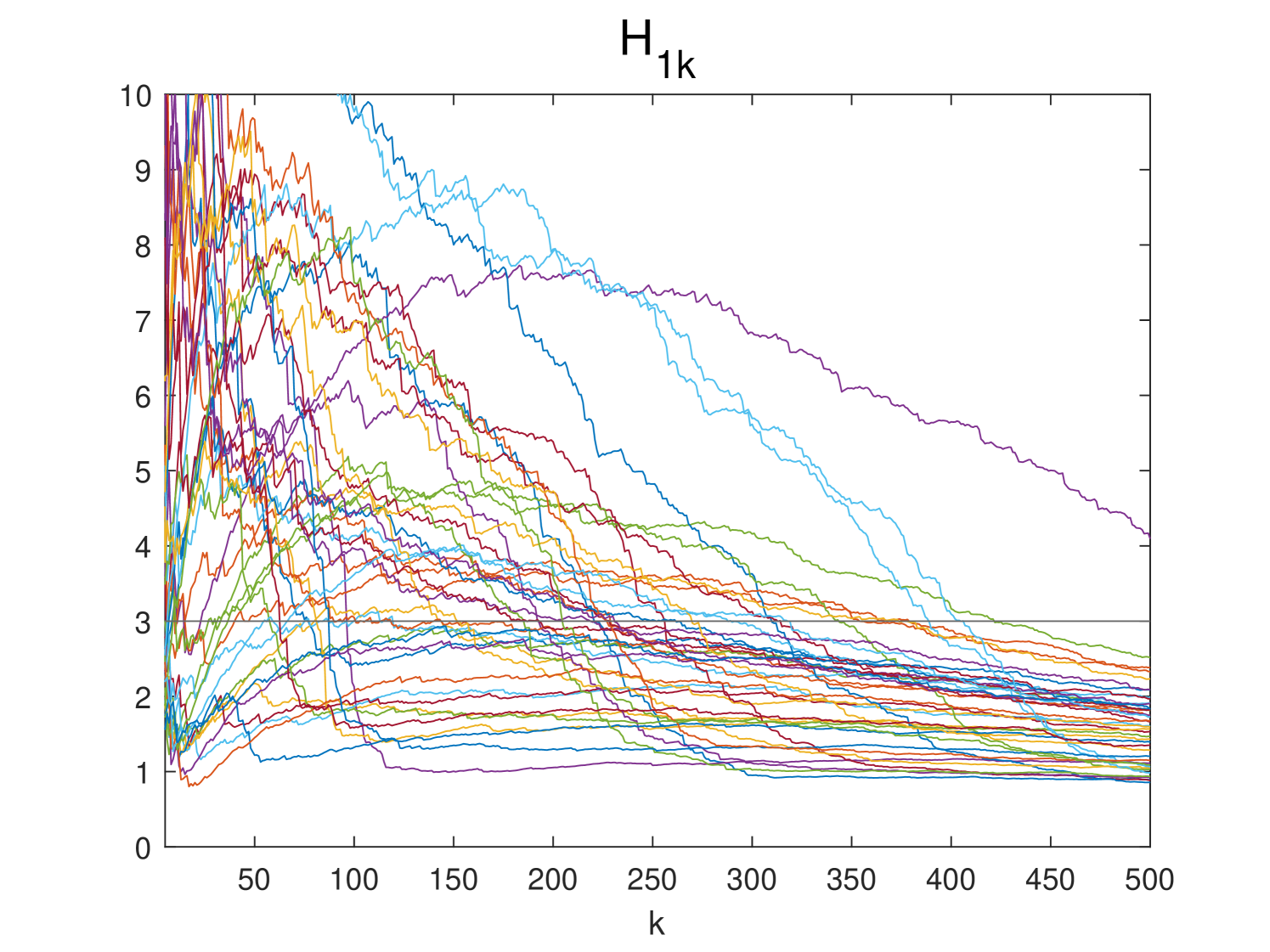
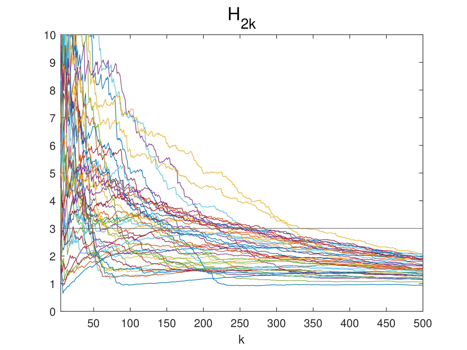
To illustrate the necessity of robust estimation method proposed in this paper, we use the Hill’s estimator to estimate the tail index of a sequence, see Hill, (1975). Specifically, let Y(i),jY_{(i),j} be the ascending order statistics of the jjth individual (coordinate) across 2215 observations. For j=1,2,,43j=1,2,\cdots,43, we give the left-tail and right-tail Hill estimators by

H1k,j={1ki=1klog(Y(i),jY(k+1),j)}1 and H2k,j={1ki=1klog(Y(ni+1),jY(nk),j)}1,H_{1k,j}=\left\{\frac{1}{k}\sum_{i=1}^{k}\log\left(\frac{Y_{(i),j}}{Y_{(k+1),j}}\right)\right\}^{-1}\quad\text{ and }\quad H_{2k,j}=\left\{\frac{1}{k}\sum_{i=1}^{k}\log\left(\frac{Y_{(n-i+1),j}}{Y_{(n-k),j}}\right)\right\}^{-1},

respectively, and they are plotted in Figure 2. From the plot, we see that most of the right-tail and the left-tail indices are below 3, suggesting the data is very likely heavy-tailed.

Refer to caption
Refer to caption
Figure 2: Hill’s estimator for 43 individuals.

We take the first 200 loci for our SBS-SN(s) change-point estimation following the practice in Zhang et al., (2021), where the decay rate for generation of seeded interval in SBS is 21/42^{-1/4}. We also compare the results obtained for Adaptive WBS-SN in Zhang et al., (2021) and 20 most significant points detected by INSPECT in Wang and Samworth, (2018). For this dataset, INSPECT is more like a screening method as it delivers a total of 67 change-points. In contrast to Adaptive WBS-SN and INSPECT where the thresholds for change-point estimation are simulated, the threshold used in SBS-SN(s) can be pre-specified, and it reflects a researcher’s confidence in detecting the change-points. We set the p-value threshold ζp\zeta_{p} as 0.001, 0.005 and 0.01 and the results are as follows:

Adaptive WBS-SN15,32,38,44,59,74,91,97,102,116,134,158,173,186,191INSPECT15,26,28,33,36,40,56,73,91,97,102,119,131,134,135,146,155,174,180,191SBS-SN(s)ζp=0.00130,41,72,89,130,136,174SBS-SN(s)ζp=0.00530,41,56,72,89,97,116,130,136,155,174,191SBS-SN(s)ζp=0.0130,41,56,72,89,97,111,116,130,136,155,174,191\begin{array}[]{ll}\text{Adaptive WBS-SN}&15,32,38,44,59,74,91,97,102,116,134,158,173,186,191\\ \text{INSPECT}&15,26,28,33,36,40,56,73,91,97,102,119,131,134,135,146,155,\\ &174,180,191\\ \text{SBS-SN${}^{(s)}$, $\zeta_{p}=0.001$}&30,41,72,89,130,136,174\\ \text{SBS-SN${}^{(s)}$, $\zeta_{p}=0.005$}&30,41,56,72,89,97,116,130,136,155,174,191\\ \text{SBS-SN${}^{(s)}$, $\zeta_{p}=0.01$}&30,41,56,72,89,97,111,116,130,136,155,174,191\end{array}

As we see, increasing the p-value threshold ζp\zeta_{p} leads to more estimated change-points, and the set of estimated change-points by using larger ζp\zeta_{p} contain those by smaller ζp\zeta_{p} as subsets. In addition, increasing ζp\zeta_{p} from 0.005 to 0.01 only brings in one more estimated change-point, suggesting ζp=0.005\zeta_{p}=0.005 may be a reasonable choice for the ACGH dataset.

All of our detected change-points at ζp=0.005\zeta_{p}=0.005 are also detected by INSPECT, i.e., 30(28), 41(40), 56, 72(73), 89(91), 97, 116, 130(131), 136 (134,135), 155, 174, 191. Although most of these points also coincide with Adaptive WBS-SN, there are non-overlapping ones. For example, 41, 56, 130 in SBS-SN(s) seem to be missed in Adaptive WBS-SN while 102 is missed by our SBS-SN(s) as it is detected by both Adaptive WBS-SN and INSPECT. These results are not really in conflict as Adaptive WBS-SN targets both sparse and dense alternatives, whereas our procedure aims to detect dense change with robustness properties.

7 Conclusion

In this paper, we propose a new method for testing and estimation of change-points in high dimensional independent data. Our test statistic builds on two recent advances in high-dimensional testing problem: spatial sign used in two-sample testing in Chakraborty and Chaudhuri, (2017) and self-normalized U-statistics in Wang et al., (2022), and inherits many advantages therein such as robustness to heavy-tailedness and tuning-free. The test is theoretically justified under both fixed-nn asymptotics and sequential asymptotics, and under both null and alternatives. When data exhibits stronger dependence in coordinates, we further enhance the analysis by focusing on RSRM models, and discover that using spatial sign leads to power improvement compared with mean based tests in Wang et al., (2022). As for multiple change-point estimation, we propose to combine p-values under the fixed-nn asymptotics with the SBS algorithm. Numerical simulations demonstrate that our fixed-nn asymptotics for spatial sign based test provides a better approximation to the finite sample distribution, and the estimation algorithm outperforms the mean-based ones when data is heavy-tailed and when coordinates are strongly dependent.

To conclude, we mention a few interesting topics for future research. Our method builds on spatial sign and targets dense signals by constructing unbiased estimators for 𝔼S(Y1Yn)\|\mathbb{E}S(Y_{1}-Y_{n})\|. As pointed out by Liu et al., (2020), many real data exhibit both sparse and dense changes, and it would be interesting to combine with the adaptive SN based test in Zhang et al., (2021) to achieve both robustness and adaptiveness. In addition, the independence assumption imposed in this paper may limit its applicability to high dimensional time series where temporal dependence can not be neglected. It’s desirable to relax the independence assumption by U-statistics based on trimmed observations, as is adopted in Wang et al., (2022). It would also be interesting to develop robust methods for detecting change-points in other quantities beyond mean, such as quantiles, covariance matrices and parameter vectors in high dimensional linear models.

Supplement to “Robust Inference for Change Points in High Dimension”


This supplementary material contains all the technical proofs for the main paper. Section S.1 contains all the proofs of main theorems and Section S.2 contains auxiliary lemmas and their proofs.

In what follows, let ai,ka_{i,k} denote the kkth coordinate of a vector aia_{i}. Denote anbna_{n}\lesssim b_{n} if there exits M,C>0M,C>0 such that anCbna_{n}\leq Cb_{n} for n>Mn>M.

S.1 Proofs of Theorems

S.1.1 Proof of Theorem 3.1

First, we have that

YiYj2==1p(Xi,Xj,)2+2(μjμi)(XjXi)+μiμj2.\displaystyle\|Y_{i}-Y_{j}\|^{2}=\sum_{\ell=1}^{p}(X_{i,\ell}-X_{j,\ell})^{2}+2(\mu_{j}-\mu_{i})^{\prime}(X_{j}-X_{i})+\|\mu_{i}-\mu_{j}\|^{2}. (S.8)

(i) Under H0H_{0}, by Theorem 8.2.2 in Lin and Lu, (2010), as pp\to\infty, we have almost surely,

1pYiYj2=2σ2.\displaystyle\frac{1}{p}\|Y_{i}-Y_{j}\|^{2}=2\sigma^{2}. (S.9)

Then, for any fixed k,l,mk,l,m, we have that

D(s)(k;l,m)=lj1,j3kj1j3k+1j2,j4mj2j4(Yj1Yj2)(Yj3Yj4)2pσ2+lj1,j3kj1j3k+1j2,j4mj2j4(Yj1Yj2)(Yj3Yj4)2pσ2{2pσ2Yj1Yj2Yj3Yj41}=:(2pσ2)1[D1(k;l,m)+D2(k;l,m)],\displaystyle\begin{split}&D^{(s)}(k;l,m)\\ =&\sum_{\begin{subarray}{c}l\leq j_{1},j_{3}\leq k\\ j_{1}\neq j_{3}\end{subarray}}\sum_{\begin{subarray}{c}k+1\leq j_{2},j_{4}\leq m\\ j_{2}\neq j_{4}\end{subarray}}\frac{(Y_{j_{1}}-Y_{j_{2}})^{\prime}(Y_{j_{3}}-Y_{j_{4}})}{2p\sigma^{2}}\\ &+\sum_{\begin{subarray}{c}l\leq j_{1},j_{3}\leq k\\ j_{1}\neq j_{3}\end{subarray}}\sum_{\begin{subarray}{c}k+1\leq j_{2},j_{4}\leq m\\ j_{2}\neq j_{4}\end{subarray}}\frac{(Y_{j_{1}}-Y_{j_{2}})^{\prime}(Y_{j_{3}}-Y_{j_{4}})}{2p\sigma^{2}}\Big{\{}\frac{2p\sigma^{2}}{\|Y_{j_{1}}-Y_{j_{2}}\|\|Y_{j_{3}}-Y_{j_{4}}\|}-1\Big{\}}\\ =:&(2p\sigma^{2})^{-1}[D_{1}(k;l,m)+D_{2}(k;l,m)],\end{split} (S.10)

where clearly D1(k;l,m)=D(k;l,m)D_{1}(k;l,m)=D(k;l,m), and

D2(k;l,m)=lj1,j3kj1j3k+1j2,j4mj2j4(Yj1Yj2)(Yj3Yj4){2pσ2Yj1Yj2Yj3Yj41}.\displaystyle D_{2}(k;l,m)=\sum_{\begin{subarray}{c}l\leq j_{1},j_{3}\leq k\\ j_{1}\neq j_{3}\end{subarray}}\sum_{\begin{subarray}{c}k+1\leq j_{2},j_{4}\leq m\\ j_{2}\neq j_{4}\end{subarray}}{(Y_{j_{1}}-Y_{j_{2}})^{\prime}(Y_{j_{3}}-Y_{j_{4}})}\Big{\{}\frac{2p\sigma^{2}}{\|Y_{j_{1}}-Y_{j_{2}}\|\|Y_{j_{3}}-Y_{j_{4}}\|}-1\Big{\}}.

Then, Theorem 4.0.1 in Lin and Lu, (2010) implies that

Γ1/2(k;l,m){D1(k;l,m)}(mk)(mk1)(kl+1)(kl)𝒟𝒩(0,1),\frac{\Gamma^{-1/2}(k;l,m)\Big{\{}D_{1}(k;l,m)\Big{\}}}{(m-k)(m-k-1)(k-l+1)(k-l)}\overset{\mathcal{D}}{\rightarrow}\mathcal{N}(0,1),

where Γ(k;l,m)=2[(ml)(ml1)](mk)(mk1)(kl+1)(kl)tr(Σ2)\Gamma(k;l,m)=\frac{2[(m-l)(m-l-1)]}{(m-k)(m-k-1)(k-l+1)(k-l)}\mathrm{tr}(\Sigma^{2}), or equivalently

1n3ΣF{D1(k;l,m)}𝒟𝒩(0,16(ml2)(kl+12)(mk2)n6).\displaystyle\frac{1}{n^{3}\|\Sigma\|_{F}}\Big{\{}D_{1}(k;l,m)\Big{\}}\overset{\mathcal{D}}{\rightarrow}\mathcal{N}\Big{(}0,\frac{16{m-l\choose 2}{k-l+1\choose 2}{m-k\choose 2}}{n^{6}}\Big{)}. (S.11)

Next, since we view nn as fixed, then for all j1j3j_{1}\neq j_{3}, j3j4j_{3}\neq j_{4}, by Theorem 4.0.1 in Lin and Lu, (2010), it follows that ΣF1(Yj1Yj2)(Yj3Yj4)=Op(1)\|\Sigma\|_{F}^{-1}(Y_{j_{1}}-Y_{j_{2}})^{\prime}(Y_{j_{3}}-Y_{j_{4}})=O_{p}(1). In addition, in view of (S.9) we have 2pσ2Yj1Yj2Yj3Yj41=op(1)\frac{2p\sigma^{2}}{\|Y_{j_{1}}-Y_{j_{2}}\|\|Y_{j_{3}}-Y_{j_{4}}\|}-1=o_{p}(1), and this implies that n3ΣF1D2(k;l,m)=op(1)n^{-3}\|\Sigma\|_{F}^{-1}D_{2}(k;l,m)=o_{p}(1).

Hence, combined with (S.11), we have

Tn(s)=supk=4,,n4(2pσ2n3ΣF1D(s)(k;1,n))24pσ4n6ΣF2Wn(s)(k;1,n)=sup4,,n4n6ΣF2[D1(k;1,n)+D2(k;1,n)]2n6ΣF2Wn(k;1,n)+op(1)=Tn+op(1),\displaystyle\begin{split}T_{n}^{(s)}=&\sup_{k=4,\cdots,n-4}\frac{\Big{(}2p\sigma^{2}n^{-3}\|\Sigma\|_{F}^{-1}D^{(s)}(k;1,n)\Big{)}^{2}}{4p\sigma^{4}n^{-6}\|\Sigma\|_{F}^{-2}W_{n}^{(s)}(k;1,n)}\\ =&\sup_{4,\cdots,n-4}\frac{n^{-6}\|\Sigma\|_{F}^{-2}[D_{1}(k;1,n)+D_{2}(k;1,n)]^{2}}{n^{-6}\|\Sigma\|_{F}^{-2}W_{n}(k;1,n)}+o_{p}(1)\\ =&T_{n}+o_{p}(1),\end{split} (S.12)

where the last equality holds since n3ΣF1D2(k;l,m)=op(1)n^{-3}\|\Sigma\|_{F}^{-1}D_{2}(k;l,m)=o_{p}(1) for each triplet (k,l,m)(k,l,m).

For 0k<mn0\leq k<m\leq n, we let

Z(k,m)=i=k+1mj=ki1XiXj,Z(k,m)=\sum_{i=k+1}^{m}\sum_{j=k}^{i-1}X_{i}^{\prime}X_{j},

then it follows that

D(k;l,m)=2(mk)(mk1)Z(l,k)+2(kl+1)(kl)Z(k+1,m)2(kl)(mk1)[Z(l,m)Z(l,k)Z(k+1,m)].\displaystyle\begin{split}D(k;l,m)=&2(m-k)(m-k-1)Z(l,k)+2(k-l+1)(k-l)Z(k+1,m)\\ &-2(k-l)(m-k-1)[Z(l,m)-Z(l,k)-Z(k+1,m)].\end{split} (S.13)

Then, by Lemma S.2.1, and continuous mapping theorem, we have

Tn𝒟supk=4,,n4nGn2(kn;1n,1)t=2k1Gn2(tn;1n,kn)+t=k+2n2Gn2(tn;k+1n,1).T_{n}\overset{\mathcal{D}}{\rightarrow}\sup_{k=4,\cdots,n-4}\frac{nG_{n}^{2}(\frac{k}{n};\frac{1}{n},1)}{\sum_{t=2}^{k-1}G_{n}^{2}(\frac{t}{n};\frac{1}{n},\frac{k}{n})+\sum_{t=k+2}^{n-2}G_{n}^{2}(\frac{t}{n};\frac{k+1}{n},1)}.

(ii) The proof is a simplified version of the proof of Theorem 3.4 (ii), hence omitted here.

S.1.2 Proof of Theorem 3.2

Clearly,

Tn(s)=supk=4,,n4(D(s)(k;1,n))2Wn(s)(k;1,n)(D(s)(k;1,n))2Wn(s)(k;1,n),T_{n}^{(s)}=\sup_{k=4,\cdots,n-4}\frac{(D^{(s)}(k;1,n))^{2}}{W_{n}^{(s)}(k;1,n)}\geq\frac{(D^{(s)}(k^{*};1,n))^{2}}{W_{n}^{(s)}(k^{*};1,n)},

and

Tn=supk=4,,n4(D(k;1,n))2Wn(k;1,n)(D(k;1,n))2Wn(k;1,n),T_{n}=\sup_{k=4,\cdots,n-4}\frac{(D(k;1,n))^{2}}{W_{n}(k;1,n)}\geq\frac{(D(k^{*};1,n))^{2}}{W_{n}(k^{*};1,n)},

Note that Wn(s)(k;1,n)=1nt=2k2D(s)(t;1,k)2+1nt=k+2n2D(s)(t;k+1,n)2.W_{n}^{(s)}(k;1,n)=\frac{1}{n}\sum_{t=2}^{k^{*}-2}D^{(s)}(t;1,k^{*})^{2}+\frac{1}{n}\sum_{t=k^{*}+2}^{n-2}D^{(s)}(t;k^{*}+1,n)^{2}. The construction of D(s)(t;1,k)2D^{(s)}(t;1,k^{*})^{2} (or D(s)(t;k+1,n)2D^{(s)}(t;k^{*}+1,n)^{2}) only uses sample before (or after) the change point, so the change point has no influence on this part. The proof of Theorem 3.1 indicates that 4p2n6ΣF2Wn(s)(k;1,n)=Op(1)4p^{2}n^{-6}\|\Sigma\|_{F}^{-2}W_{n}^{(s)}(k;1,n)=O_{p}(1) and similarly 4n6ΣF2Wn(k;1,n)=Op(1)4n^{-6}\|\Sigma\|_{F}^{-2}W_{n}(k;1,n)=O_{p}(1). Hence, it suffices to show pn3ΣF1D(s)(k;1,n)ppn^{-3}\|\Sigma\|_{F}^{-1}D^{(s)}(k^{*};1,n)\to_{p}\infty and n3ΣF1D(k;1,n)pn^{-3}\|\Sigma\|_{F}^{-1}D(k^{*};1,n)\to_{p}\infty.

Denote δi\delta_{i} as the iith element of δ\delta. By (S.8), for 1j1j3k1\leq j_{1}\neq j_{3}\leq k^{*} and k+1j2j4nk^{*}+1\leq j_{2}\neq j_{4}\leq n,

p1Yj1Yj22=\displaystyle p^{-1}\|Y_{j_{1}}-Y_{j_{2}}\|^{2}= p1δ2+p1i=1p(Xj1,iXj2,i)2p1i=1p2δi(Xj1,iXj2,i),\displaystyle p^{-1}\|\delta\|^{2}+p^{-1}\sum_{i=1}^{p}(X_{j_{1},i}-X_{j_{2},i})^{2}-p^{-1}\sum_{i=1}^{p}2\delta_{i}(X_{j_{1},i}-X_{j_{2},i}),
p1Yj3Yj42=\displaystyle p^{-1}\|Y_{j_{3}}-Y_{j_{4}}\|^{2}= p1δ2+p1i=1p(Xj3,iXj4,i)2p1i=1p2δi(Xj3,iXj4,i),\displaystyle p^{-1}\|\delta\|^{2}+p^{-1}\sum_{i=1}^{p}(X_{j_{3},i}-X_{j_{4},i})^{2}-p^{-1}\sum_{i=1}^{p}2\delta_{i}(X_{j_{3},i}-X_{j_{4},i}),

and

p1(Yj1Yj2)(Yj3Yj4)=\displaystyle p^{-1}(Y_{j_{1}}-Y_{j_{2}})^{\prime}(Y_{j_{3}}-Y_{j_{4}})= p1δ2+p1i=1p(Xj1,iXj2,i)(Xj3,iXj4,i)\displaystyle p^{-1}\|\delta\|^{2}+p^{-1}\sum_{i=1}^{p}(X_{j_{1},i}-X_{j_{2},i})(X_{j_{3},i}-X_{j_{4},i})
p1i=1pδi(Xj1,iXj2,i)p1i=1pδi(Xj3,iXj4,i).\displaystyle-p^{-1}\sum_{i=1}^{p}\delta_{i}(X_{j_{1},i}-X_{j_{2},i})-p^{-1}\sum_{i=1}^{p}\delta_{i}(X_{j_{3},i}-X_{j_{4},i}).

Using Theorem 8.2.2 in Lin and Lu, (2010), and the independence of XiX_{i}’s, we have

p1Yj1Yj22pι2+2σ2,\displaystyle p^{-1}\|Y_{j_{1}}-Y_{j_{2}}\|^{2}\to_{p}\iota^{2}+2\sigma^{2},
p1Yj3Yj42pι2+2σ2,\displaystyle p^{-1}\|Y_{j_{3}}-Y_{j_{4}}\|^{2}\to_{p}\iota^{2}+2\sigma^{2},

and

p1(Yj1Yj2)(Yj3Yj4)pι2.\displaystyle p^{-1}(Y_{j_{1}}-Y_{j_{2}})^{\prime}(Y_{j_{3}}-Y_{j_{4}})\to_{p}\iota^{2}.

If ι>0\iota>0, then

n4D(s)(k;1,n)pn4k(k1)(nk)(nk1)ι2ι2+2σ2>0,n^{-4}D^{(s)}(k^{*};1,n)\to_{p}n^{-4}k^{*}(k^{*}-1)(n-k^{*})(n-k^{*}-1)\frac{\iota^{2}}{\iota^{2}+2\sigma^{2}}>0,

and

p1n4D(k;1,n)pn4(k)(k1)(nk)(nk1)ι2>0.p^{-1}n^{-4}D(k^{*};1,n)\to_{p}n^{-4}(k^{*})(k^{*}-1)(n-k^{*})(n-k^{*}-1)\iota^{2}>0.

Hence,

pn3ΣF1D(s)(k;1,n)=(pnΣF1)n4D(s)(k;1,n)p,pn^{-3}\|\Sigma\|_{F}^{-1}D^{(s)}(k^{*};1,n)=(pn\|\Sigma\|_{F}^{-1})n^{-4}D^{(s)}(k^{*};1,n)\to_{p}\infty,

and

n3ΣF1D(k;1,n)=(pnΣF1)p1n4D(k;1,n)p.n^{-3}\|\Sigma\|_{F}^{-1}D(k^{*};1,n)=(pn\|\Sigma\|_{F}^{-1})p^{-1}n^{-4}D(k^{*};1,n)\to_{p}\infty.

S.1.3 Proof of Theorem 3.3

By symmetry, we only consider the case l<kk<ml<k\leq k^{*}<m. Since under Assumption 3.4, (S.9) still holds by Cauchy-Schwartz inequality, then using similar arguments in the proof of Theorem 3.1, we have

2pσ2D(s)(k;l,m)=lj1,j3kj1j3k+1j2,j4mj2j4(Xj1Xj2)(Xj3Xj4)(1+o(1))+(kl+1)(kl)(mk)(mk1)δ2(1+o(1))(2(kl)(mk)(mk2)j=lkXjδ+4(kl)(kl1)(mk)j=k+1kXjδ)(1+o(1)):=D(1)(s)(k;l,m)+D(2)(s)(k;l,m)D(3)(s)(k;l,m).\displaystyle\begin{split}&2p\sigma^{2}D^{(s)}(k;l,m)\\ =&\sum_{\begin{subarray}{c}l\leq j_{1},j_{3}\leq k\\ j_{1}\neq j_{3}\end{subarray}}\sum_{\begin{subarray}{c}k+1\leq j_{2},j_{4}\leq m\\ j_{2}\neq j_{4}\end{subarray}}(X_{j_{1}}-X_{j_{2}})^{\prime}(X_{j_{3}}-X_{j_{4}})(1+o(1))\\ &+(k-l+1)(k-l)(m-k^{*})(m-k^{*}-1)\|\delta\|^{2}(1+o(1))\\ &-\Big{(}2(k-l)(m-k^{*})(m-k-2)\sum_{j=l}^{k}X_{j}^{\prime}\delta+4(k-l)(k-l-1)(m-k^{*})\sum_{j=k+1}^{k^{*}}X_{j}^{\prime}\delta\Big{)}(1+o(1))\\ :=&D^{(s)}_{(1)}(k;l,m)+D^{(s)}_{(2)}(k;l,m)-D^{(s)}_{(3)}(k;l,m).\end{split} (S.14)

That is, 2pσ2D(s)(k;l,m)=D(k;l,m)(1+o(1))2p\sigma^{2}D^{(s)}(k;l,m)=D(k;l,m)(1+o(1)) for any triplet (k,l,m)(k,l,m), hence it suffices to consider Tn(s)T_{n}^{(s)} as the results of TnT_{n} are similar.

We first note that

Var(Xiδ)=δΣδ=o(ΣF2),\mathrm{Var}(X_{i}^{\prime}\delta)=\delta^{\prime}\Sigma\delta=o(\|\Sigma\|_{F}^{2}),

hence by Chebyshev inequality, for any triplet (k,l,m)(k,l,m), we have

n3ΣF1D(3)(s)(k;l,m)=op(1).n^{-3}\|\Sigma\|_{F}^{-1}D^{(s)}_{(3)}(k;l,m)=o_{p}(1). (S.15)

(i) By similar arguments in the proof of Theorem 3.2, it suffices to show

2pσ2n3ΣF1D(s)(k;1,n)p.2p\sigma^{2}n^{-3}\|\Sigma\|_{F}^{-1}D^{(s)}(k^{*};1,n)\to_{p}\infty.

In fact, by similar arguments used in the proof of Theorem 3.1, we can show that

n3ΣF1D(1)(s)(k;l,m)=Op(1).n^{-3}\|\Sigma\|_{F}^{-1}D^{(s)}_{(1)}(k;l,m)=O_{p}(1).

Then, recall (S.14), the result follows by noting

n3ΣF1D(2)(s)(k;1,n)=n3ΣF1(kl+1)(kl)(mk)(mk1)δ2(1+o(1)).n^{-3}\|\Sigma\|_{F}^{-1}D^{(s)}_{(2)}\left(k^{*};1,n\right)=n^{-3}\|\Sigma\|_{F}^{-1}(k-l+1)(k-l)\left(m-k^{*}\right)\left(m-k^{*}-1\right)\|\delta\|^{2}(1+o(1))\rightarrow\infty.

(ii) As nΣF1δ20n\|\Sigma\|_{F}^{-1}\|\delta\|^{2}\to 0, it follows from the same argument as (S.12).

(iii) As nΣF1δ2cn(0,)n\|\Sigma\|_{F}^{-1}\|\delta\|^{2}\to c_{n}\in(0,\infty), then we have

n3ΣF1D(2)(s)(k;m,l)]\displaystyle n^{-3}\|\Sigma\|_{F}^{-1}D^{(s)}_{(2)}(k^{*};m,l)]
=\displaystyle= n3ΣF1(kl+1)(kl)(mk)(mk1)δ2(1+o(1))\displaystyle n^{-3}\|\Sigma\|_{F}^{-1}(k-l+1)(k-l)(m-k^{*})(m-k^{*}-1)\|\delta\|^{2}(1+o(1))
\displaystyle\to cn4(kl+12)(mk2)n4.\displaystyle c_{n}\frac{4{k-l+1\choose 2}{m-k^{*}\choose 2}}{n^{4}}.

Therefore, continuous mapping theorem together with Lemma S.2.1 indicate that

Tn(s)𝒟supk=4,,n4n[2Gn(kn;1n,1)+cnΔn(kn;1n,1)]2t=2k2[2Gn(tn;1n,kn)+cnΔn(tn;1n,kn)]2+t=k+2n2[2Gn(tn;k+1n,1)+cnΔn(tn;k+1n,1)]2.T_{n}^{(s)}\overset{\mathcal{D}}{\rightarrow}\sup_{k=4,\cdots,n-4}\frac{n[\sqrt{2}G_{n}(\frac{k}{n};\frac{1}{n},1)+c_{n}\Delta_{n}(\frac{k}{n};\frac{1}{n},1)]^{2}}{\sum_{t=2}^{k-2}[\sqrt{2}G_{n}(\frac{t}{n};\frac{1}{n},\frac{k}{n})+c_{n}\Delta_{n}(\frac{t}{n};\frac{1}{n},\frac{k}{n})]^{2}+\sum_{t=k+2}^{n-2}[\sqrt{2}G_{n}(\frac{t}{n};\frac{k+1}{n},1)+c_{n}\Delta_{n}(\frac{t}{n};\frac{k+1}{n},1)]^{2}}.

The last part of the proof is similar to the proof of Theorem 3.5 (ii) below, and is simpler, hence omitted.

S.1.4 Proof of Theorem 3.4

(i) Note that

1pYiYj2=1p=1p(Xi,RiXj,Rj)2,\frac{1}{p}\|Y_{i}-Y_{j}\|^{2}=\frac{1}{p}\sum_{\ell=1}^{p}(\frac{X_{i,\ell}}{R_{i}}-\frac{X_{j,\ell}}{R_{j}})^{2}, (S.16)

hence given n\mathcal{R}_{n}, as pp\to\infty, we have almost surely

1pYiYj2σ2(Ri2+Rj2).\frac{1}{p}\|Y_{i}-Y_{j}\|^{2}\to\sigma^{2}(R_{i}^{-2}+R_{j}^{-2}). (S.17)

Note that

pσ2D(s)(k;l,m)=lj1,j3kj1j3k+1j2,j4mj2j4(Yj1Yj2)(Yj3Yj4)(Rj12+Rj22)1/2(Rj32+Rj42)1/2+lj1,j3kj1j3k+1j2,j4mj2j4(Yj1Yj2)(Yj3Yj4)(Rj12+Rj22)1/2(Rj32+Rj42)1/2{pσ2(Rj12+Rj22)1/2(Rj32+Rj42)1/2Yj1Yj2Yj3Yj41}=:[D3(k;l,m)+D4(k;l,m)].\displaystyle\begin{split}&p\sigma^{2}D^{(s)}(k;l,m)\\ =&\sum_{\begin{subarray}{c}l\leq j_{1},j_{3}\leq k\\ j_{1}\neq j_{3}\end{subarray}}\sum_{\begin{subarray}{c}k+1\leq j_{2},j_{4}\leq m\\ j_{2}\neq j_{4}\end{subarray}}\frac{(Y_{j_{1}}-Y_{j_{2}})^{\prime}(Y_{j_{3}}-Y_{j_{4}})}{(R_{j_{1}}^{-2}+R_{j_{2}}^{-2})^{1/2}(R_{j_{3}}^{-2}+R_{j_{4}}^{-2})^{1/2}}\\ &+\sum_{\begin{subarray}{c}l\leq j_{1},j_{3}\leq k\\ j_{1}\neq j_{3}\end{subarray}}\sum_{\begin{subarray}{c}k+1\leq j_{2},j_{4}\leq m\\ j_{2}\neq j_{4}\end{subarray}}\frac{(Y_{j_{1}}-Y_{j_{2}})^{\prime}(Y_{j_{3}}-Y_{j_{4}})}{(R_{j_{1}}^{-2}+R_{j_{2}}^{-2})^{1/2}(R_{j_{3}}^{-2}+R_{j_{4}}^{-2})^{1/2}}\Big{\{}\frac{p\sigma^{2}(R_{j_{1}}^{-2}+R_{j_{2}}^{-2})^{1/2}(R_{j_{3}}^{-2}+R_{j_{4}}^{-2})^{1/2}}{\|Y_{j_{1}}-Y_{j_{2}}\|\|Y_{j_{3}}-Y_{j_{4}}\|}-1\Big{\}}\\ =:&[D_{3}(k;l,m)+D_{4}(k;l,m)].\end{split} (S.18)

Let

Aj1,j3(k;l,m)=\displaystyle A_{j_{1},j_{3}}(k;l,m)= k+1j2,j4mj2j4(Rj12+Rj22)1/2(Rj32+Rj42)1/2,\displaystyle\sum_{\begin{subarray}{c}k+1\leq j_{2},j_{4}\leq m\\ j_{2}\neq j_{4}\end{subarray}}(R_{j_{1}}^{-2}+R_{j_{2}}^{-2})^{-1/2}(R_{j_{3}}^{-2}+R_{j_{4}}^{-2})^{-1/2},
Bj2,j4(k;l,m)=\displaystyle B_{j_{2},j_{4}}(k;l,m)= lj1,j3kj1j3(Rj12+Rj22)1/2(Rj32+Rj42)1/2,\displaystyle\sum_{\begin{subarray}{c}l\leq j_{1},j_{3}\leq k\\ j_{1}\neq j_{3}\end{subarray}}(R_{j_{1}}^{-2}+R_{j_{2}}^{-2})^{-1/2}(R_{j_{3}}^{-2}+R_{j_{4}}^{-2})^{-1/2},

and

Cj1,j2(k;l,m)=\displaystyle C_{j_{1},j_{2}}(k;l,m)= 2lj3kj3j1k+1j4mj4j2(Rj12+Rj22)1/2(Rj32+Rj42)1/2.\displaystyle-2\sum_{\begin{subarray}{c}l\leq j_{3}\leq k\\ j_{3}\neq j_{1}\end{subarray}}\sum_{\begin{subarray}{c}k+1\leq j_{4}\leq m\\ j_{4}\neq j_{2}\end{subarray}}(R_{j_{1}}^{-2}+R_{j_{2}}^{-2})^{-1/2}(R_{j_{3}}^{-2}+R_{j_{4}}^{-2})^{-1/2}.

Then under H0H_{0},

D3(k;l,m)\displaystyle D_{3}(k;l,m)
=\displaystyle= lj1,j3kj1j3Xj1TXj3(Rj1Rj3)1Aj1,j3(k;l,m)+k+1j2,j4mj2j4Xj2TXj4(Rj2Rj4)1Bj2,j4(k;l,m)\displaystyle\sum_{\begin{subarray}{c}l\leq j_{1},j_{3}\leq k\\ j_{1}\neq j_{3}\end{subarray}}X_{j_{1}}^{T}X_{j_{3}}(R_{j_{1}}R_{j_{3}})^{-1}A_{j_{1},j_{3}}(k;l,m)+\sum_{\begin{subarray}{c}k+1\leq j_{2},j_{4}\leq m\\ j_{2}\neq j_{4}\end{subarray}}X_{j_{2}}^{T}X_{j_{4}}(R_{j_{2}}R_{j_{4}})^{-1}B_{j_{2},j_{4}}(k;l,m)
+lj1kk+1j2mXj1TXj2(Rj1Rj2)1Cj1,j2(k;l,m).\displaystyle+\sum_{l\leq j_{1}\leq k}\sum_{k+1\leq j_{2}\leq m}X_{j_{1}}^{T}X_{j_{2}}(R_{j_{1}}R_{j_{2}})^{-1}C_{j_{1},j_{2}}(k;l,m).

Denote that U1=(X1TX2,,X1TXn,X2TX3,,X2TXn,,Xn1TXn)TU_{1}=(X_{1}^{T}X_{2},...,X_{1}^{T}X_{n},X_{2}^{T}X_{3},...,X_{2}^{T}X_{n},...,X_{n-1}^{T}X_{n})^{T} which contains all inner products of XiX_{i} and XjX_{j} for all iji\neq j, and U2=(R1,,Rn)TU_{2}=(R_{1},...,R_{n})^{T}. By definition, σ(U1)σ(U2)\sigma(U_{1})\perp\!\!\!\perp\sigma(U_{2}), where σ(U)\sigma(U) is the σ\sigma-field generated by UU, and we further observe that 2pσ2D3(k;l,m)2p\sigma^{2}D_{3}(k;l,m) is a continuous functional of U1U_{1} and U2U_{2}. Hence to derive the limiting distribution of 2pσ2D3(k;l,m)2p\sigma^{2}D_{3}(k;l,m) when pp\rightarrow\infty, it suffices to derive the limiting distribution of (U1,U2)T(U_{1},U_{2})^{T}.

For any αn(n1)/2\alpha\in\mathbb{R}^{n(n-1)/2}, similar to the proof of Theorem 3.1, by Theorem 4.0.1 in Lin and Lu, (2010) we have

ΣF1αTU1𝒟αT𝒵:=αT(𝒵1,2,𝒵1,3,,𝒵1,n,𝒵2,3,,𝒵2,n,,𝒵n1,n)T,\|\Sigma\|_{F}^{-1}\alpha^{T}U_{1}\overset{\mathcal{D}}{\rightarrow}\alpha^{T}\mathcal{Z}:=\alpha^{T}(\mathcal{Z}_{1,2},\mathcal{Z}_{1,3},...,\mathcal{Z}_{1,n},\mathcal{Z}_{2,3},...,\mathcal{Z}_{2,n},...,\mathcal{Z}_{n-1,n})^{T},

where 𝒵1,2,,𝒵n1,n\mathcal{Z}_{1,2},...,\mathcal{Z}_{n-1,n} are i.i.d. standard normal random variables, and we can assume 𝒵\mathcal{Z} is independent of U2U_{2}. For the ease of our notation, we let 𝒵i,j=𝒵j,i\mathcal{Z}_{i,j}=\mathcal{Z}_{j,i}, for all i>ji>j. Furthermore since σ(U1)σ(U2)\sigma(U_{1})\perp\!\!\!\perp\sigma(U_{2}), for any αn(n1)/2\alpha\in\mathbb{R}^{n(n-1)/2} and βn\beta\in\mathbb{R}^{n}, the characteristic function of αTU1+βTU2\alpha^{T}U_{1}+\beta^{T}U_{2} is the product of the characteristic function of αTU1\alpha^{T}U_{1} and that of βTU2\beta^{T}U_{2}. By applying the Cramér-Wold device, (ΣF1U1,U2)𝒟(𝒵,U2)(\|\Sigma\|_{F}^{-1}U_{1},U_{2})\overset{\mathcal{D}}{\rightarrow}(\mathcal{Z},U_{2}). Therefore, by continuous mapping theorem, as pp\rightarrow\infty,

n3ΣF1D3(k;l,m)𝒟Gn(n,s)(k/n;l/n,m/n),n^{-3}\|\Sigma\|_{F}^{-1}D_{3}(k;l,m)\overset{\mathcal{D}}{\rightarrow}G_{n}^{(\mathcal{R}_{n},s)}(k/n;l/n,m/n), (S.19)

where

Gn(n,s)(k/n;l/n,m/n):=n3lj1,j3kj1j3𝒵j1,j3(Rj1Rj3)1Aj1,j3(k,l,m)+n3k+1j2,j4mj2j4𝒵j2,j4(Rj2Rj4)1Bj2,j4(k,l,m)+n3lj1kk+1j2m𝒵j1,j2(Rj1Rj2)1Cj1,j2(k,l,m).\displaystyle\begin{split}&G_{n}^{(\mathcal{R}_{n},s)}(k/n;l/n,m/n)\\ :=&n^{-3}\sum_{\begin{subarray}{c}l\leq j_{1},j_{3}\leq k\\ j_{1}\neq j_{3}\end{subarray}}\mathcal{Z}_{j_{1},j_{3}}(R_{j_{1}}R_{j_{3}})^{-1}A_{j_{1},j_{3}}(k,l,m)+n^{-3}\sum_{\begin{subarray}{c}k+1\leq j_{2},j_{4}\leq m\\ j_{2}\neq j_{4}\end{subarray}}\mathcal{Z}_{j_{2},j_{4}}(R_{j_{2}}R_{j_{4}})^{-1}B_{j_{2},j_{4}}(k,l,m)\\ &+n^{-3}\sum_{l\leq j_{1}\leq k}\sum_{k+1\leq j_{2}\leq m}\mathcal{Z}_{j_{1},j_{2}}(R_{j_{1}}R_{j_{2}})^{-1}C_{j_{1},j_{2}}(k,l,m).\end{split} (S.20)

It is clear that the conditional distribution of Gn(n,s)(k/n;l/n,m/n)G_{n}^{(\mathcal{R}_{n},s)}(k/n;l/n,m/n) given n\mathcal{R}_{n} is Gaussian, and for any l1<k1<m1,l2<k2<m2l_{1}<k_{1}<m_{1},l_{2}<k_{2}<m_{2}, k1,k2,l1,l2,m1,m2=1,2,,nk_{1},k_{2},l_{1},l_{2},m_{1},m_{2}=1,2,...,n, the covariance structure is given by

Cov(Gn(n,s)(k1/n;l1/n,m1/n),Gn(n,s)(k2/n;l2/n,m2/n)|n)\displaystyle\mathrm{Cov}(G_{n}^{(\mathcal{R}_{n},s)}(k_{1}/n;l_{1}/n,m_{1}/n),G_{n}^{(\mathcal{R}_{n},s)}(k_{2}/n;l_{2}/n,m_{2}/n)|\mathcal{R}_{n}) (S.21)
=\displaystyle= 2n6{(l1l2)j1,j2(k1k2)j1j2Rj12Rj22Aj1,j2(k1;l1,m1)Aj1,j2(k2;l2,m2)\displaystyle 2n^{-6}\Big{\{}\sum_{\begin{subarray}{c}(l_{1}\lor l_{2})\leq j_{1},j_{2}\leq(k_{1}\land k_{2})\\ j_{1}\neq j_{2}\end{subarray}}R_{j_{1}}^{-2}R_{j_{2}}^{-2}A_{j_{1},j_{2}}(k_{1};l_{1},m_{1})A_{j_{1},j_{2}}(k_{2};l_{2},m_{2})
+(l1k2+1)j1,j2(k1m2)j1j2Rj12Rj22Aj1,j2(k1;l1,m1)Bj1,j2(k2;l2,m2)\displaystyle+\sum_{\begin{subarray}{c}(l_{1}\lor k_{2}+1)\leq j_{1},j_{2}\leq(k_{1}\land m_{2})\\ j_{1}\neq j_{2}\end{subarray}}R_{j_{1}}^{-2}R_{j_{2}}^{-2}A_{j_{1},j_{2}}(k_{1};l_{1},m_{1})B_{j_{1},j_{2}}(k_{2};l_{2},m_{2})
+2j1=(l1l2)k2j2=k2+1(m2k1)𝟏(k1>k2)Rj12Rj22Aj1,j2(k1;l1,m1)Cj1,j2(k2;l2,m2)\displaystyle+2\sum_{j_{1}=(l_{1}\lor l_{2})}^{k_{2}}\sum_{j_{2}=k_{2}+1}^{(m_{2}\land k_{1})}\mathbf{1}(k_{1}>k_{2})R_{j_{1}}^{-2}R_{j_{2}}^{-2}A_{j_{1},j_{2}}(k_{1};l_{1},m_{1})C_{j_{1},j_{2}}(k_{2};l_{2},m_{2})
+(k1+1l2)j1,j2(m1k2)j1j2Rj12Rj22Bj1,j2(k1;l1,m1)Aj1,j2(k2;l2,m2)\displaystyle+\sum_{\begin{subarray}{c}(k_{1}+1\lor l_{2})\leq j_{1},j_{2}\leq(m_{1}\land k_{2})\\ j_{1}\neq j_{2}\end{subarray}}R_{j_{1}}^{-2}R_{j_{2}}^{-2}B_{j_{1},j_{2}}(k_{1};l_{1},m_{1})A_{j_{1},j_{2}}(k_{2};l_{2},m_{2})
+(k1+1k2+1)j1,j2(m1m2)j1j2Rj12Rj22Bj1,j2(k1;l1,m1)Bj1,j24(k2;l2,m2)\displaystyle+\sum_{\begin{subarray}{c}(k_{1}+1\lor k_{2}+1)\leq j_{1},j_{2}\leq(m_{1}\land m_{2})\\ j_{1}\neq j_{2}\end{subarray}}R_{j_{1}}^{-2}R_{j_{2}}^{-2}B_{j_{1},j_{2}}(k_{1};l_{1},m_{1})B_{j_{1},j_{2}4}(k_{2};l_{2},m_{2})
+2j1=(k1+1l2)k2j2=k2+1(m1m2)𝟏(m1>k2)Rj12Rj22Bj1,j2(k1;l1,m1)Cj1,j2(k2;l2,m2)\displaystyle+2\sum_{j_{1}=(k_{1}+1\lor l_{2})}^{k_{2}}\sum_{j_{2}=k_{2}+1}^{(m_{1}\land m_{2})}\mathbf{1}(m_{1}>k_{2})R_{j_{1}}^{-2}R_{j_{2}}^{-2}B_{j_{1},j_{2}}(k_{1};l_{1},m_{1})C_{j_{1},j_{2}}(k_{2};l_{2},m_{2})
+2j1=(l1l2)k1j2=k1+1(m1k2)𝟏(k2>k1)Rj12Rj22Cj1,j2(k1;l1,m1)Aj1,j2(k2;l2,m2)\displaystyle+2\sum_{j_{1}=(l_{1}\lor l_{2})}^{k_{1}}\sum_{j_{2}=k_{1}+1}^{(m_{1}\land k_{2})}\mathbf{1}(k_{2}>k_{1})R_{j_{1}}^{-2}R_{j_{2}}^{-2}C_{j_{1},j_{2}}(k_{1};l_{1},m_{1})A_{j_{1},j_{2}}(k_{2};l_{2},m_{2})
+2j1=(k2+1l1)k1j2=k1+1(m1m2)𝟏(m2>k1)Rj12Rj22Cj1,j2(k1;l1,m1)Bj1,j2(k2;l2,m2)\displaystyle+2\sum_{j_{1}=(k_{2}+1\lor l_{1})}^{k_{1}}\sum_{j_{2}=k_{1}+1}^{(m_{1}\land m_{2})}\mathbf{1}(m_{2}>k_{1})R_{j_{1}}^{-2}R_{j_{2}}^{-2}C_{j_{1},j_{2}}(k_{1};l_{1},m_{1})B_{j_{1},j_{2}}(k_{2};l_{2},m_{2})
+j1=(l1l2)(k1k2)j2=(k1+1k2+1)(m1m2)Rj12Rj22Cj1,j2(k1;l1,m1)Cj1,j2(k2;l2,m2)}.\displaystyle+\sum_{j_{1}=(l_{1}\lor l_{2})}^{(k_{1}\land k_{2})}\sum_{j_{2}=(k_{1}+1\lor k_{2}+1)}^{(m_{1}\land m_{2})}R_{j_{1}}^{-2}R_{j_{2}}^{-2}C_{j_{1},j_{2}}(k_{1};l_{1},m_{1})C_{j_{1},j_{2}}(k_{2};l_{2},m_{2})\Big{\}}.

Clearly, when Ri1R_{i}\equiv 1, we have 2D3(k;l,m)=D1(k;l,m)2D_{3}(k;l,m)=D_{1}(k;l,m) where D1(k;l,m)D_{1}(k;l,m) is defined in (S.10), and the result reduces to (S.11).

Using (S.17), we can see that given n\mathcal{R}_{n}, D4(k;l,m)n3ΣF=op(1)\frac{D_{4}(k;l,m)}{n^{3}\|\Sigma\|_{F}}=o_{p}(1). Hence, given n\mathcal{R}_{n}, we have

Tn(s)=supk=4,,n4[D3(k;1,n)]21nt=l+1k2D3(t;l,k)2+1nt=k+2m2D3(t;k+1,m)2+op(1).T_{n}^{(s)}=\sup_{k=4,\cdots,n-4}\frac{[D_{3}(k;1,n)]^{2}}{\frac{1}{n}\sum_{t=l+1}^{k-2}D_{3}(t;l,k)^{2}+\frac{1}{n}\sum_{t=k+2}^{m-2}D_{3}(t;k+1,m)^{2}}+o_{p}(1).

Then, by (S.19), we have that as pp\to\infty,

Tn(s)|n𝒟𝒯n(n,s):=supk=4,,n4n[Gn(n,s)(k/n;1/n,1)]2t=2k1[Gn(n,s)(t/n;1/n,k/n)]2+t=k+2n2[Gn(n,s)(t/n;(k+1)/n,1)]2.T_{n}^{(s)}|\mathcal{R}_{n}\overset{\mathcal{D}}{\rightarrow}\mathcal{T}_{n}^{(\mathcal{R}_{n},s)}:=\sup_{k=4,\cdots,n-4}\frac{n[G_{n}^{(\mathcal{R}_{n},s)}(k/n;1/n,1)]^{2}}{\sum_{t=2}^{k-1}[G_{n}^{(\mathcal{R}_{n},s)}(t/n;1/n,k/n)]^{2}+\sum_{t=k+2}^{n-2}[G_{n}^{(\mathcal{R}_{n},s)}(t/n;(k+1)/n,1)]^{2}}.

As for TnT_{n}, note that

D(k;l,m)=\displaystyle D(k;l,m)= (mk)(mk1)lj1,j3kj1j3Xj1TXj3(Rj1Rj3)1\displaystyle(m-k)(m-k-1)\sum_{\begin{subarray}{c}l\leq j_{1},j_{3}\leq k\\ j_{1}\neq j_{3}\end{subarray}}X_{j_{1}}^{T}X_{j_{3}}(R_{j_{1}}R_{j_{3}})^{-1}
+(kl+1)(kl)k+1j2,j4mj2j4Xj2TXj4(Rj2Rj4)1\displaystyle+(k-l+1)(k-l)\sum_{\begin{subarray}{c}k+1\leq j_{2},j_{4}\leq m\\ j_{2}\neq j_{4}\end{subarray}}X_{j_{2}}^{T}X_{j_{4}}(R_{j_{2}}R_{j_{4}})^{-1}
2(kl)(mk1)lj1kk+1j2mXj1TXj2(Rj1Rj2)1.\displaystyle-2(k-l)(m-k-1)\sum_{l\leq j_{1}\leq k}\sum_{k+1\leq j_{2}\leq m}X_{j_{1}}^{T}X_{j_{2}}(R_{j_{1}}R_{j_{2}})^{-1}.

Using similar arguments as in (S.19), we have

n3ΣF1D(k;l,m)𝒟Gn(n)(k/n;l/n,m/n),n^{-3}\|\Sigma\|_{F}^{-1}D(k;l,m)\overset{\mathcal{D}}{\rightarrow}G_{n}^{(\mathcal{R}_{n})}(k/n;l/n,m/n), (S.22)

where

Gn(n)(k/n;l/n,m/n)=(mk)(mk1)n3lj1,j3kj1j3𝒵j1,j3(Rj1Rj3)1+(kl+1)(kl)n3k+1j2,j4mj2j4𝒵j2,j4(Rj2Rj4)12(kl)(mk1)n3lj1kk+1j2m𝒵j1,j2(Rj1Rj2)1.\displaystyle\begin{split}G_{n}^{(\mathcal{R}_{n})}(k/n;l/n,m/n)=&(m-k)(m-k-1)n^{-3}\sum_{\begin{subarray}{c}l\leq j_{1},j_{3}\leq k\\ j_{1}\neq j_{3}\end{subarray}}\mathcal{Z}_{j_{1},j_{3}}(R_{j_{1}}R_{j_{3}})^{-1}\\ &+(k-l+1)(k-l)n^{-3}\sum_{\begin{subarray}{c}k+1\leq j_{2},j_{4}\leq m\\ j_{2}\neq j_{4}\end{subarray}}\mathcal{Z}_{j_{2},j_{4}}(R_{j_{2}}R_{j_{4}})^{-1}\\ &-2(k-l)(m-k-1)n^{-3}\sum_{l\leq j_{1}\leq k}\sum_{k+1\leq j_{2}\leq m}\mathcal{Z}_{j_{1},j_{2}}(R_{j_{1}}R_{j_{2}})^{-1}.\end{split} (S.23)

Similar to Gn(n,s)(k/n;l/n,m/n)G_{n}^{(\mathcal{R}_{n},s)}(k/n;l/n,m/n), the conditional distribution of Gn(n)(k/n;l/n,m/n)G_{n}^{(\mathcal{R}_{n})}(k/n;l/n,m/n) given n\mathcal{R}_{n} is Gaussian, and for any l1<k1<m1,l2<k2<m2l_{1}<k_{1}<m_{1},l_{2}<k_{2}<m_{2}, k1,k2,l1,l2,m1,m2=1,2,,nk_{1},k_{2},l_{1},l_{2},m_{1},m_{2}=1,2,...,n, the covariance structure is given by

Cov(Gn(n)(k1/n;l1/n,m1/n),Gn(n)(k2/n;l2/n,m2/n)|n)\displaystyle\mathrm{Cov}(G_{n}^{(\mathcal{R}_{n})}(k_{1}/n;l_{1}/n,m_{1}/n),G_{n}^{(\mathcal{R}_{n})}(k_{2}/n;l_{2}/n,m_{2}/n)|\mathcal{R}_{n}) (S.24)
=\displaystyle= 8n6{(l1l2)j1,j2(k1k2)j1j2Rj12Rj22(m1k12)(m2k22)\displaystyle 8n^{-6}\Big{\{}\sum_{\begin{subarray}{c}(l_{1}\lor l_{2})\leq j_{1},j_{2}\leq(k_{1}\land k_{2})\\ j_{1}\neq j_{2}\end{subarray}}R_{j_{1}}^{-2}R_{j_{2}}^{-2}{m_{1}-k_{1}\choose 2}{m_{2}-k_{2}\choose 2}
+(l1k2+1)j1,j2(k1m2)j1j2Rj12Rj22(m1k12)(k1l1+12)\displaystyle+\sum_{\begin{subarray}{c}(l_{1}\lor k_{2}+1)\leq j_{1},j_{2}\leq(k_{1}\land m_{2})\\ j_{1}\neq j_{2}\end{subarray}}R_{j_{1}}^{-2}R_{j_{2}}^{-2}{m_{1}-k_{1}\choose 2}{k_{1}-l_{1}+1\choose 2}
2j1=(l1l2)k2j2=k2+1(m2k1)𝟏(k1>k2)Rj12Rj22(m1k12)(k2l2)(m2k21)\displaystyle-2\sum_{j_{1}=(l_{1}\lor l_{2})}^{k_{2}}\sum_{j_{2}=k_{2}+1}^{(m_{2}\land k_{1})}\mathbf{1}(k_{1}>k_{2})R_{j_{1}}^{-2}R_{j_{2}}^{-2}{m_{1}-k_{1}\choose 2}(k_{2}-l_{2})(m_{2}-k_{2}-1)
+(k1+1l2)j1,j2(m1k2)j1j2Rj12Rj22(k1l1+12)(m2k22)\displaystyle+\sum_{\begin{subarray}{c}(k_{1}+1\lor l_{2})\leq j_{1},j_{2}\leq(m_{1}\land k_{2})\\ j_{1}\neq j_{2}\end{subarray}}R_{j_{1}}^{-2}R_{j_{2}}^{-2}{k_{1}-l_{1}+1\choose 2}{m_{2}-k_{2}\choose 2}
+(k1+1k2+1)j1,j2(m1m2)j1j2Rj12Rj22(k1l1+12)(k2l2+12)\displaystyle+\sum_{\begin{subarray}{c}(k_{1}+1\lor k_{2}+1)\leq j_{1},j_{2}\leq(m_{1}\land m_{2})\\ j_{1}\neq j_{2}\end{subarray}}R_{j_{1}}^{-2}R_{j_{2}}^{-2}{k_{1}-l_{1}+1\choose 2}{k_{2}-l_{2}+1\choose 2}
2j1=(k1+1l2)k2j2=k2+1(m1m2)𝟏(m1>k2)Rj12Rj22Bj1,j2(k1l1+12)(k2l2)(m2k21)\displaystyle-2\sum_{j_{1}=(k_{1}+1\lor l_{2})}^{k_{2}}\sum_{j_{2}=k_{2}+1}^{(m_{1}\land m_{2})}\mathbf{1}(m_{1}>k_{2})R_{j_{1}}^{-2}R_{j_{2}}^{-2}B_{j_{1},j_{2}}{k_{1}-l_{1}+1\choose 2}(k_{2}-l_{2})(m_{2}-k_{2}-1)
2j1=(l1l2)k1j2=k1+1(m1k2)𝟏(k2>k1)Rj12Rj22(k1l1)(m1k11)(m2k22)\displaystyle-2\sum_{j_{1}=(l_{1}\lor l_{2})}^{k_{1}}\sum_{j_{2}=k_{1}+1}^{(m_{1}\land k_{2})}\mathbf{1}(k_{2}>k_{1})R_{j_{1}}^{-2}R_{j_{2}}^{-2}(k_{1}-l_{1})(m_{1}-k_{1}-1){m_{2}-k_{2}\choose 2}
2j1=(k2+1l1)k1j2=k1+1(m1m2)𝟏(m2>k1)Rj12Rj22(k1l1)(m1k11)(k2l2+12)\displaystyle-2\sum_{j_{1}=(k_{2}+1\lor l_{1})}^{k_{1}}\sum_{j_{2}=k_{1}+1}^{(m_{1}\land m_{2})}\mathbf{1}(m_{2}>k_{1})R_{j_{1}}^{-2}R_{j_{2}}^{-2}(k_{1}-l_{1})(m_{1}-k_{1}-1){k_{2}-l_{2}+1\choose 2}
+j1=(l1l2)(k1k2)j2=(k1+1k2+1)(m1m2)Rj12Rj22(k1l1)(m1k11)(k2l2)(m2k21)}.\displaystyle+\sum_{j_{1}=(l_{1}\lor l_{2})}^{(k_{1}\land k_{2})}\sum_{j_{2}=(k_{1}+1\lor k_{2}+1)}^{(m_{1}\land m_{2})}R_{j_{1}}^{-2}R_{j_{2}}^{-2}(k_{1}-l_{1})(m_{1}-k_{1}-1)(k_{2}-l_{2})(m_{2}-k_{2}-1)\Big{\}}.

Hence, as pp\to\infty,

Tn|n𝒟𝒯n(n):=supk=4,,n4n[Gn(n)(k/n;1/n,1)]2t=2k1[Gn(n)(t/n;1/n,k/n)]2+t=k+2n2[Gn(n)(t/n;(k+1)/n,1)]2.T_{n}|\mathcal{R}_{n}\overset{\mathcal{D}}{\rightarrow}\mathcal{T}_{n}^{(\mathcal{R}_{n})}:=\sup_{k=4,\cdots,n-4}\frac{n[G_{n}^{(\mathcal{R}_{n})}(k/n;1/n,1)]^{2}}{\sum_{t=2}^{k-1}[G_{n}^{(\mathcal{R}_{n})}(t/n;1/n,k/n)]^{2}+\sum_{t=k+2}^{n-2}[G_{n}^{(\mathcal{R}_{n})}(t/n;(k+1)/n,1)]^{2}}.

(ii)

We shall only show the process convergence Gn(n,s)()𝔼[R1R2(R12+R32)(R22+R32)]2G()G_{n}^{(\mathcal{R}_{n},s)}(\cdot)\rightsquigarrow\mathbb{E}\Big{[}\frac{R_{1}R_{2}}{\sqrt{(R_{1}^{2}+R_{3}^{2})(R_{2}^{2}+R_{3}^{2})}}\Big{]}\sqrt{2}G(\cdot). That Gn(n)()𝔼(R12)2G()G_{n}^{(\mathcal{R}_{n})}(\cdot)\rightsquigarrow\mathbb{E}(R_{1}^{-2})\sqrt{2}G(\cdot) is similar and simpler. Once the process convergence is obtained, the limiting distributions of 𝒯n(n,s)\mathcal{T}_{n}^{(\mathcal{R}_{n},s)} and 𝒯n(n)\mathcal{T}_{n}^{(\mathcal{R}_{n})} can be easily obtained by the continuous mapping theorem.

The proof for the process convergence contains two parts: the finite dimensional convergence and the tightness.

To show the finite dimensional convergence, we need to show that for any positive integer NN, any fixed u1,u2,,uN[0,1]3u_{1},u_{2},...,u_{N}\in[0,1]^{3} and any α1,,αN\alpha_{1},...,\alpha_{N}\in\mathbb{R},

α1Gn(n,s)(u1)+αNGn(n,s)(uN)𝒟𝔼2[R1R2(R12+R32)(R22+R32)]2[α1G(u1)+αNG(uN)],\alpha_{1}G_{n}^{(\mathcal{R}_{n},s)}(u_{1})+\cdots\alpha_{N}G_{n}^{(\mathcal{R}_{n},s)}(u_{N})\overset{\mathcal{D}}{\rightarrow}\mathbb{E}^{2}\Big{[}\frac{R_{1}R_{2}}{\sqrt{(R_{1}^{2}+R_{3}^{2})(R_{2}^{2}+R_{3}^{2})}}\Big{]}\sqrt{2}[\alpha_{1}G(u_{1})+\cdots\alpha_{N}G(u_{N})],

where for u=(u(1),u(2),u(3))Tu=(u^{(1)},u^{(2)},u^{(3)})^{T}, Gn(u)=Gn(u1;u2,u3)G_{n}(u)=G_{n}(u_{1};u_{2},u_{3}). Since both Gn(n,s)()|nG_{n}^{(\mathcal{R}_{n},s)}(\cdot)|\mathcal{R}_{n} and G()G(\cdot) are Gaussian processes, by Lemma S.2.2 we have

P(α1Gn(n,s)(u1)+αkGn(n,s)(uk)<x|n)\displaystyle P(\alpha_{1}G_{n}^{(\mathcal{R}_{n},s)}(u_{1})+\cdots\alpha_{k}G_{n}^{(\mathcal{R}_{n},s)}(u_{k})<x|\mathcal{R}_{n})
p\displaystyle\to_{p} P(𝔼[R1R2(R12+R32)(R22+R32)]2[α1G(u1)+αNG(uN)]<x).\displaystyle P(\mathbb{E}\Big{[}\frac{R_{1}R_{2}}{\sqrt{(R_{1}^{2}+R_{3}^{2})(R_{2}^{2}+R_{3}^{2})}}\Big{]}\sqrt{2}[\alpha_{1}G(u_{1})+\cdots\alpha_{N}G(u_{N})]<x).

Then by bounded convergence theorem we have

limnP(α1Gn(n,s)(u1)+αkGn(n,s)(uk)<x)\displaystyle\lim_{n\rightarrow\infty}P(\alpha_{1}G_{n}^{(\mathcal{R}_{n},s)}(u_{1})+\cdots\alpha_{k}G_{n}^{(\mathcal{R}_{n},s)}(u_{k})<x)
=\displaystyle= limn𝔼[P(α1Gn(n,s)(u1)+αkGn(n,s)(uk)<x|n)]\displaystyle\lim_{n\rightarrow\infty}\mathbb{E}[P(\alpha_{1}G_{n}^{(\mathcal{R}_{n},s)}(u_{1})+\cdots\alpha_{k}G_{n}^{(\mathcal{R}_{n},s)}(u_{k})<x|\mathcal{R}_{n})]
=\displaystyle= 𝔼[limnP(α1Gn(n,s)(u1)+αkGn(n,s)(uk)<x|n)]\displaystyle\mathbb{E}[\lim_{n\rightarrow\infty}P(\alpha_{1}G_{n}^{(\mathcal{R}_{n},s)}(u_{1})+\cdots\alpha_{k}G_{n}^{(\mathcal{R}_{n},s)}(u_{k})<x|\mathcal{R}_{n})]
=\displaystyle= 𝔼[R1R2(R12+R32)(R22+R32)]2[α1G(u1)+αkG(uk)]<x)]\displaystyle\mathbb{E}\Big{[}\frac{R_{1}R_{2}}{\sqrt{(R_{1}^{2}+R_{3}^{2})(R_{2}^{2}+R_{3}^{2})}}\Big{]}\sqrt{2}[\alpha_{1}G(u_{1})+\cdots\alpha_{k}G(u_{k})]<x)]
=\displaystyle= P(𝔼[R1R2(R12+R32)(R22+R32)]2[α1G(u1)+αkG(uk)]<x).\displaystyle P(\mathbb{E}\Big{[}\frac{R_{1}R_{2}}{\sqrt{(R_{1}^{2}+R_{3}^{2})(R_{2}^{2}+R_{3}^{2})}}\Big{]}\sqrt{2}[\alpha_{1}G(u_{1})+\cdots\alpha_{k}G(u_{k})]<x).

This completes the proof of the finite dimensional convergence.

To show the tightness, it suffices to show that there exists C>0C>0 such that

𝔼[(Gn(n,s)(u)Gn(n,s)(v))8]C(uv4+1/n4),\mathbb{E}[(G_{n}^{(\mathcal{R}_{n},s)}(u)-G_{n}^{(\mathcal{R}_{n},s)}(v))^{8}]\leq C(\|u-v\|^{4}+1/n^{4}),

for any u,v[0,1]3u,v\in[0,1]^{3} (see the proof of equation S8.12 in Wang et al., (2022)).

Since given n\mathcal{R}_{n}, Gn(n,s)()G_{n}^{(\mathcal{R}_{n},s)}(\cdot) is a Gaussian process, we have

𝔼[(Gn(n,s)(u)Gn(n,s)(v))8]=𝔼[𝔼[(Gn(n,s)(u)Gn(n,s)(v))8|n]]\displaystyle\mathbb{E}[(G_{n}^{(\mathcal{R}_{n},s)}(u)-G_{n}^{(\mathcal{R}_{n},s)}(v))^{8}]=\mathbb{E}[\mathbb{E}[(G_{n}^{(\mathcal{R}_{n},s)}(u)-G_{n}^{(\mathcal{R}_{n},s)}(v))^{8}|\mathcal{R}_{n}]]
=C𝔼[Var((Gn(n,s)(u)Gn(n,s)(v))|n)4].\displaystyle=C\mathbb{E}[\mathrm{Var}((G_{n}^{(\mathcal{R}_{n},s)}(u)-G_{n}^{(\mathcal{R}_{n},s)}(v))|\mathcal{R}_{n})^{4}].

By (S.21), for u=(k1/n,l1/n,m1/n)u=(k_{1}/n,l_{1}/n,m_{1}/n) (and similar for v=(k2/n,l2/n,m2/n)v=(k_{2}/n,l_{2}/n,m_{2}/n)) this reduces to

Var(Gn(n,s)(u)|n)\displaystyle\mathrm{Var}(G_{n}^{(\mathcal{R}_{n},s)}(u)|\mathcal{R}_{n})
=\displaystyle= 2n6{l1j1,j3k1j1j3(Rj1Rj3)2Aj1,j3(k1,l1,m1)2+k1+1j2,j4m1j2j4(Rj2Rj4)2Bj2,j4(k1,l1,m1)2\displaystyle 2n^{-6}\Big{\{}\sum_{\begin{subarray}{c}l_{1}\leq j_{1},j_{3}\leq k_{1}\\ j_{1}\neq j_{3}\end{subarray}}(R_{j_{1}}R_{j_{3}})^{-2}A_{j_{1},j_{3}}(k_{1},l_{1},m_{1})^{2}+\sum_{\begin{subarray}{c}k_{1}+1\leq j_{2},j_{4}\leq m_{1}\\ j_{2}\neq j_{4}\end{subarray}}(R_{j_{2}}R_{j_{4}})^{-2}B_{j_{2},j_{4}}(k_{1},l_{1},m_{1})^{2}
+l1j1k1k1+1j2m1(Rj1Rj2)2Cj1,j2(k1,l1,m1)2}.\displaystyle+\sum_{l_{1}\leq j_{1}\leq k_{1}}\sum_{k_{1}+1\leq j_{2}\leq m_{1}}(R_{j_{1}}R_{j_{2}})^{-2}C_{j_{1},j_{2}}(k_{1},l_{1},m_{1})^{2}\Big{\}}.

Note that

𝔼[(Gn(n,s)(k1/n;l1/n,m1/n)Gn(n,s)(k2/n;l2/n,m2/n))8]\displaystyle\mathbb{E}[(G_{n}^{(\mathcal{R}_{n},s)}(k_{1}/n;l_{1}/n,m_{1}/n)-G_{n}^{(\mathcal{R}_{n},s)}(k_{2}/n;l_{2}/n,m_{2}/n))^{8}]
\displaystyle\lesssim 𝔼[(Gn(n,s)(k1/n;l1/n,m1/n)Gn(n,s)(k2/n;l1/n,m1/n))8]\displaystyle\mathbb{E}[(G_{n}^{(\mathcal{R}_{n},s)}(k_{1}/n;l_{1}/n,m_{1}/n)-G_{n}^{(\mathcal{R}_{n},s)}(k_{2}/n;l_{1}/n,m_{1}/n))^{8}]
+𝔼[(Gn(n,s)(k2/n;l1/n,m1/n)Gn(n,s)(k2/n;l2/n,m1/n))8]\displaystyle+\mathbb{E}[(G_{n}^{(\mathcal{R}_{n},s)}(k_{2}/n;l_{1}/n,m_{1}/n)-G_{n}^{(\mathcal{R}_{n},s)}(k_{2}/n;l_{2}/n,m_{1}/n))^{8}]
+𝔼[(Gn(n,s)(k2/n;l2/n,m1/n)Gn(n,s)(k2/n;l2/n,m2/n))8]\displaystyle+\mathbb{E}[(G_{n}^{(\mathcal{R}_{n},s)}(k_{2}/n;l_{2}/n,m_{1}/n)-G_{n}^{(\mathcal{R}_{n},s)}(k_{2}/n;l_{2}/n,m_{2}/n))^{8}]
=\displaystyle= I1+I2+I3.\displaystyle I_{1}+I_{2}+I_{3}.

We shall analyze I1I_{1} first, and WLOG we let k1<k2k_{1}<k_{2}. Then we have (with l1=l2,m1=m2l_{1}=l_{2},m_{1}=m_{2})

Cov(Gn(n,s)(k1/n;l1/n,m1/n),Gn(n,s)(k2/n;l2/n,m2/n)|n)\displaystyle\mathrm{Cov}(G_{n}^{(\mathcal{R}_{n},s)}(k_{1}/n;l_{1}/n,m_{1}/n),G_{n}^{(\mathcal{R}_{n},s)}(k_{2}/n;l_{2}/n,m_{2}/n)|\mathcal{R}_{n})
=\displaystyle= 2n6{l1j1,j3k1j1j3Rj12Rj32Aj1,j3(k1;l1,m1)Aj1,j3(k2;l1,m1)\displaystyle 2n^{-6}\Big{\{}\sum_{\begin{subarray}{c}l_{1}\leq j_{1},j_{3}\leq k_{1}\\ j_{1}\neq j_{3}\end{subarray}}R_{j_{1}}^{-2}R_{j_{3}}^{-2}A_{j_{1},j_{3}}(k_{1};l_{1},m_{1})A_{j_{1},j_{3}}(k_{2};l_{1},m_{1})
+k1+1j1,j2k2j1j2Rj12Rj22Bj1,j2(k1;l1,m1)Aj1,j2(k2;l2,m2)\displaystyle+\sum_{\begin{subarray}{c}k_{1}+1\leq j_{1},j_{2}\leq k_{2}\\ j_{1}\neq j_{2}\end{subarray}}R_{j_{1}}^{-2}R_{j_{2}}^{-2}B_{j_{1},j_{2}}(k_{1};l_{1},m_{1})A_{j_{1},j_{2}}(k_{2};l_{2},m_{2})
+k2+1j2,j4m1j2j4Rj22Rj42Bj2,j4(k1;l1,m1)Bj2,j4(k2;l2,m2)\displaystyle+\sum_{\begin{subarray}{c}k_{2}+1\leq j_{2},j_{4}\leq m_{1}\\ j_{2}\neq j_{4}\end{subarray}}R_{j_{2}}^{-2}R_{j_{4}}^{-2}B_{j_{2},j_{4}}(k_{1};l_{1},m_{1})B_{j_{2},j_{4}}(k_{2};l_{2},m_{2})
+2j1=k1+1k2j2=k2+1m1Rj12Rj22Cj1,j2(k2;l2,m2)Bj1,j2(k1;l1,m1)\displaystyle+2\sum_{j_{1}=k_{1}+1}^{k_{2}}\sum_{j_{2}=k_{2}+1}^{m_{1}}R_{j_{1}}^{-2}R_{j_{2}}^{-2}C_{j_{1},j_{2}}(k_{2};l_{2},m_{2})B_{j_{1},j_{2}}(k_{1};l_{1},m_{1})
+2j1=l1k1j2=k1+1k2Rj12Rj22Cj1,j2(k1;l1,m1)Aj1,j2(k2;l2,m2)\displaystyle+2\sum_{j_{1}=l_{1}}^{k_{1}}\sum_{j_{2}=k_{1}+1}^{k_{2}}R_{j_{1}}^{-2}R_{j_{2}}^{-2}C_{j_{1},j_{2}}(k_{1};l_{1},m_{1})A_{j_{1},j_{2}}(k_{2};l_{2},m_{2})
+j1=l1k1j2=k2+1m1Rj12Rj22Cj1,j2(k1;l1,m1)Cj1,j2(k2;l2,m2)}.\displaystyle+\sum_{j_{1}=l_{1}}^{k_{1}}\sum_{j_{2}=k_{2}+1}^{m_{1}}R_{j_{1}}^{-2}R_{j_{2}}^{-2}C_{j_{1},j_{2}}(k_{1};l_{1},m_{1})C_{j_{1},j_{2}}(k_{2};l_{2},m_{2})\Big{\}}.

Hence,

Var(Gn(n,s)(k1/n;l1/n,m1/n)Gn(n,s)(k2/n;l2/n,m2/n)|n)\displaystyle\mathrm{Var}(G_{n}^{(\mathcal{R}_{n},s)}(k_{1}/n;l_{1}/n,m_{1}/n)-G_{n}^{(\mathcal{R}_{n},s)}(k_{2}/n;l_{2}/n,m_{2}/n)|\mathcal{R}_{n})
=\displaystyle= 2n6{l1j1,j3k1j1j3(Rj1Rj3)2Aj1,j3(k1,l1,m1)2+k1+1j2,j4m1j2j4(Rj2Rj4)2Bj2,j4(k1,l1,m1)2\displaystyle 2n^{-6}\Big{\{}\sum_{\begin{subarray}{c}l_{1}\leq j_{1},j_{3}\leq k_{1}\\ j_{1}\neq j_{3}\end{subarray}}(R_{j_{1}}R_{j_{3}})^{-2}A_{j_{1},j_{3}}(k_{1},l_{1},m_{1})^{2}+\sum_{\begin{subarray}{c}k_{1}+1\leq j_{2},j_{4}\leq m_{1}\\ j_{2}\neq j_{4}\end{subarray}}(R_{j_{2}}R_{j_{4}})^{-2}B_{j_{2},j_{4}}(k_{1},l_{1},m_{1})^{2}
+l1j1k1k1+1j2m1(Rj1Rj2)2Cj1,j2(k1,l1,m1)2}\displaystyle+\sum_{l_{1}\leq j_{1}\leq k_{1}}\sum_{k_{1}+1\leq j_{2}\leq m_{1}}(R_{j_{1}}R_{j_{2}})^{-2}C_{j_{1},j_{2}}(k_{1},l_{1},m_{1})^{2}\Big{\}}
+\displaystyle+ 2n6{l1j1,j3k2j1j3(Rj1Rj3)2Aj1,j3(k2,l1,m1)2+k2+1j2,j4m1j2j4(Rj2Rj4)2Bj2,j4(k2,l1,m1)2\displaystyle 2n^{-6}\Big{\{}\sum_{\begin{subarray}{c}l_{1}\leq j_{1},j_{3}\leq k_{2}\\ j_{1}\neq j_{3}\end{subarray}}(R_{j_{1}}R_{j_{3}})^{-2}A_{j_{1},j_{3}}(k_{2},l_{1},m_{1})^{2}+\sum_{\begin{subarray}{c}k_{2}+1\leq j_{2},j_{4}\leq m_{1}\\ j_{2}\neq j_{4}\end{subarray}}(R_{j_{2}}R_{j_{4}})^{-2}B_{j_{2},j_{4}}(k_{2},l_{1},m_{1})^{2}
+l1j1k2k2+1j2m1(Rj1Rj2)2Cj1,j2(k2,l1,m1)2}\displaystyle+\sum_{l_{1}\leq j_{1}\leq k_{2}}\sum_{k_{2}+1\leq j_{2}\leq m_{1}}(R_{j_{1}}R_{j_{2}})^{-2}C_{j_{1},j_{2}}(k_{2},l_{1},m_{1})^{2}\Big{\}}
\displaystyle- 4n6{l1j1,j3k1j1j3Rj12Rj32Aj1,j3(k1;l1,m1)Aj1,j3(k2;l1,m1)\displaystyle 4n^{-6}\Big{\{}\sum_{\begin{subarray}{c}l_{1}\leq j_{1},j_{3}\leq k_{1}\\ j_{1}\neq j_{3}\end{subarray}}R_{j_{1}}^{-2}R_{j_{3}}^{-2}A_{j_{1},j_{3}}(k_{1};l_{1},m_{1})A_{j_{1},j_{3}}(k_{2};l_{1},m_{1})
+k1+1j1,j2k2j1j2Rj12Rj22Bj1,j2(k1;l1,m1)Aj1,j2(k2;l2,m2)\displaystyle+\sum_{\begin{subarray}{c}k_{1}+1\leq j_{1},j_{2}\leq k_{2}\\ j_{1}\neq j_{2}\end{subarray}}R_{j_{1}}^{-2}R_{j_{2}}^{-2}B_{j_{1},j_{2}}(k_{1};l_{1},m_{1})A_{j_{1},j_{2}}(k_{2};l_{2},m_{2})
+k2+1j2,j4m1j2j4Rj22Rj42Bj2,j4(k1;l1,m1)Bj2,j4(k2;l2,m2)\displaystyle+\sum_{\begin{subarray}{c}k_{2}+1\leq j_{2},j_{4}\leq m_{1}\\ j_{2}\neq j_{4}\end{subarray}}R_{j_{2}}^{-2}R_{j_{4}}^{-2}B_{j_{2},j_{4}}(k_{1};l_{1},m_{1})B_{j_{2},j_{4}}(k_{2};l_{2},m_{2})
+2j1=k1+1k2j2=k2+1m1Rj12Rj22Cj1,j2(k2;l2,m2)Bj1,j2(k1;l1,m1)\displaystyle+2\sum_{j_{1}=k_{1}+1}^{k_{2}}\sum_{j_{2}=k_{2}+1}^{m_{1}}R_{j_{1}}^{-2}R_{j_{2}}^{-2}C_{j_{1},j_{2}}(k_{2};l_{2},m_{2})B_{j_{1},j_{2}}(k_{1};l_{1},m_{1})
+2j1=l1k1j2=k1+1k2Rj12Rj22Cj1,j2(k1;l1,m1)Aj1,j2(k2;l2,m2)\displaystyle+2\sum_{j_{1}=l_{1}}^{k_{1}}\sum_{j_{2}=k_{1}+1}^{k_{2}}R_{j_{1}}^{-2}R_{j_{2}}^{-2}C_{j_{1},j_{2}}(k_{1};l_{1},m_{1})A_{j_{1},j_{2}}(k_{2};l_{2},m_{2})
+j1=l1k1j2=k2+1m1Rj12Rj22Cj1,j2(k1;l1,m1)Cj1,j2(k2;l2,m2)}.\displaystyle+\sum_{j_{1}=l_{1}}^{k_{1}}\sum_{j_{2}=k_{2}+1}^{m_{1}}R_{j_{1}}^{-2}R_{j_{2}}^{-2}C_{j_{1},j_{2}}(k_{1};l_{1},m_{1})C_{j_{1},j_{2}}(k_{2};l_{2},m_{2})\Big{\}}.

By rearranging terms we have

Var(Gn(n,s)(k1/n;l1/n,m1/n)Gn(n,s)(k2/n;l2/n,m2/n)|n)\displaystyle\mathrm{Var}(G_{n}^{(\mathcal{R}_{n},s)}(k_{1}/n;l_{1}/n,m_{1}/n)-G_{n}^{(\mathcal{R}_{n},s)}(k_{2}/n;l_{2}/n,m_{2}/n)|\mathcal{R}_{n})
=\displaystyle= 2n6{l1j1,j3k1j1j3(Rj1Rj3)2(Aj1,j3(k1,l1,m1)Aj1,j3(k2,l1,m1))2\displaystyle 2n^{-6}\Big{\{}\sum_{\begin{subarray}{c}l_{1}\leq j_{1},j_{3}\leq k_{1}\\ j_{1}\neq j_{3}\end{subarray}}(R_{j_{1}}R_{j_{3}})^{-2}(A_{j_{1},j_{3}}(k_{1},l_{1},m_{1})-A_{j_{1},j_{3}}(k_{2},l_{1},m_{1}))^{2}
+j1=k1+1k2j3=l1j11(Rj1Rj3)2(Aj1,j3(k2,l1,m1)2+Aj3,j1(k2,l1,m1)2)\displaystyle+\sum_{j_{1}=k_{1}+1}^{k_{2}}\sum_{j_{3}=l_{1}}^{j_{1}-1}(R_{j_{1}}R_{j_{3}})^{-2}(A_{j_{1},j_{3}}(k_{2},l_{1},m_{1})^{2}+A_{j_{3},j_{1}}(k_{2},l_{1},m_{1})^{2})
+k2+1j2,j4m1j2j4Rj22Rj42(Bj2,j4(k1;l1,m1)Bj2,j4(k2;l1,m1))2\displaystyle+\sum_{\begin{subarray}{c}k_{2}+1\leq j_{2},j_{4}\leq m_{1}\\ j_{2}\neq j_{4}\end{subarray}}R_{j_{2}}^{-2}R_{j_{4}}^{-2}(B_{j_{2},j_{4}}(k_{1};l_{1},m_{1})-B_{j_{2},j_{4}}(k_{2};l_{1},m_{1}))^{2}
+j2=k1+1k21j4=j2+1m1Rj22Rj42(Bj2,j4(k1;l1,m1)2+Bj4,j2(k1;l1,m1)2)\displaystyle+\sum_{j_{2}=k_{1}+1}^{k_{2}-1}\sum_{j_{4}=j_{2}+1}^{m_{1}}R_{j_{2}}^{-2}R_{j_{4}}^{-2}(B_{j_{2},j_{4}}(k_{1};l_{1},m_{1})^{2}+B_{j_{4},j_{2}}(k_{1};l_{1},m_{1})^{2})
+j1=l1k1j2=k2+1m1Rj12Rj22(Cj1,j2(k1,l1,m1)Cj1,j2(k2,l1,m1))2\displaystyle+\sum_{j_{1}=l_{1}}^{k_{1}}\sum_{j_{2}=k_{2}+1}^{m_{1}}R_{j_{1}}^{-2}R_{j_{2}}^{-2}(C_{j_{1},j_{2}}(k_{1},l_{1},m_{1})-C_{j_{1},j_{2}}(k_{2},l_{1},m_{1}))^{2}
+j1=l1k1j2=k1+1k2Rj12Rj22Cj1,j2(k1,l1,m1)2+j1=k1+1k2j2=k2+1m1Rj12Rj22Cj1,j2(k2,l1,m1)2\displaystyle+\sum_{j_{1}=l_{1}}^{k_{1}}\sum_{j_{2}=k_{1}+1}^{k_{2}}R_{j_{1}}^{-2}R_{j_{2}}^{-2}C_{j_{1},j_{2}}(k_{1},l_{1},m_{1})^{2}+\sum_{j_{1}=k_{1}+1}^{k_{2}}\sum_{j_{2}=k_{2}+1}^{m_{1}}R_{j_{1}}^{-2}R_{j_{2}}^{-2}C_{j_{1},j_{2}}(k_{2},l_{1},m_{1})^{2}
2k1+1j1,j2k2j1j2Rj12Rj22Bj1,j2(k1;l1,m1)Aj1,j2(k2;l1,m1)\displaystyle-2\sum_{\begin{subarray}{c}k_{1}+1\leq j_{1},j_{2}\leq k_{2}\\ j_{1}\neq j_{2}\end{subarray}}R_{j_{1}}^{-2}R_{j_{2}}^{-2}B_{j_{1},j_{2}}(k_{1};l_{1},m_{1})A_{j_{1},j_{2}}(k_{2};l_{1},m_{1})
4j1=k1+1k2j2=k2+1m1Rj12Rj22Cj1,j2(k2;l1,m1)Bj1,j2(k1;l1,m1)\displaystyle-4\sum_{j_{1}=k_{1}+1}^{k_{2}}\sum_{j_{2}=k_{2}+1}^{m_{1}}R_{j_{1}}^{-2}R_{j_{2}}^{-2}C_{j_{1},j_{2}}(k_{2};l_{1},m_{1})B_{j_{1},j_{2}}(k_{1};l_{1},m_{1})
4j1=l1k1j2=k1+1k2Rj12Rj22Cj1,j2(k1;l1,m1)Aj1,j2(k2;l1,m1)\displaystyle-4\sum_{j_{1}=l_{1}}^{k_{1}}\sum_{j_{2}=k_{1}+1}^{k_{2}}R_{j_{1}}^{-2}R_{j_{2}}^{-2}C_{j_{1},j_{2}}(k_{1};l_{1},m_{1})A_{j_{1},j_{2}}(k_{2};l_{1},m_{1})
=\displaystyle= l=110Ji.\displaystyle\sum_{l=1}^{10}J_{i}.

Thus by CR-inequality we have I1=𝔼[(l=110Jl)4]i=110𝔼[Jl4]I_{1}=\mathbb{E}[(\sum_{l=1}^{10}J_{l})^{4}]\lesssim\sum_{i=1}^{10}\mathbb{E}[J_{l}^{4}]. We shall analyze 𝔼[J14]\mathbb{E}[J_{1}^{4}] first. Note that

Aj1,j3(k1,l1,m1)Aj1,j3(k2,l1,m1)\displaystyle A_{j_{1},j_{3}}(k_{1},l_{1},m_{1})-A_{j_{1},j_{3}}(k_{2},l_{1},m_{1})
=\displaystyle= k1+1j2,j4m1j2j4(Rj12+Rj22)1/2(Rj32+Rj42)1/2k2+1j2,j4m1j2j4(Rj12+Rj22)1/2(Rj32+Rj42)1/2\displaystyle\sum_{\begin{subarray}{c}k_{1}+1\leq j_{2},j_{4}\leq m_{1}\\ j_{2}\neq j_{4}\end{subarray}}(R_{j_{1}}^{-2}+R_{j_{2}}^{-2})^{-1/2}(R_{j_{3}}^{-2}+R_{j_{4}}^{-2})^{-1/2}-\sum_{\begin{subarray}{c}k_{2}+1\leq j_{2},j_{4}\leq m_{1}\\ j_{2}\neq j_{4}\end{subarray}}(R_{j_{1}}^{-2}+R_{j_{2}}^{-2})^{-1/2}(R_{j_{3}}^{-2}+R_{j_{4}}^{-2})^{-1/2}
=\displaystyle= j2=k1+1k2j4=j2+1m1(Rj12+Rj22)1/2(Rj32+Rj42)1/2+j4=k1+1k2j2=j4+1m1(Rj12+Rj22)1/2(Rj32+Rj42)1/2\displaystyle\sum_{j_{2}=k_{1}+1}^{k_{2}}\sum_{j_{4}=j_{2}+1}^{m_{1}}(R_{j_{1}}^{-2}+R_{j_{2}}^{-2})^{-1/2}(R_{j_{3}}^{-2}+R_{j_{4}}^{-2})^{-1/2}+\sum_{j_{4}=k_{1}+1}^{k_{2}}\sum_{j_{2}=j_{4}+1}^{m_{1}}(R_{j_{1}}^{-2}+R_{j_{2}}^{-2})^{-1/2}(R_{j_{3}}^{-2}+R_{j_{4}}^{-2})^{-1/2}
\displaystyle\leq 2j2=k1+1k2j4=j2+1m1(2|Rj1|1|Rj2|1)1/2(2|Rj3|1|Rj4|1)1/2\displaystyle 2\sum_{j_{2}=k_{1}+1}^{k_{2}}\sum_{j_{4}=j_{2}+1}^{m_{1}}(2|R_{j_{1}}|^{-1}|R_{j_{2}}|^{-1})^{-1/2}(2|R_{j_{3}}|^{-1}|R_{j_{4}}|^{-1})^{-1/2}
\displaystyle\leq |Rj1Rj3|1/2j2=k1+1k2j4=j2+1m1|Rj2Rj4|1/2.\displaystyle|R_{j_{1}}R_{j_{3}}|^{1/2}\sum_{j_{2}=k_{1}+1}^{k_{2}}\sum_{j_{4}=j_{2}+1}^{m_{1}}|R_{j_{2}}R_{j_{4}}|^{1/2}.

Since Aj1,j3(k1,l1,m1)Aj1,j3(k2,l1,m1)>0A_{j_{1},j_{3}}(k_{1},l_{1},m_{1})-A_{j_{1},j_{3}}(k_{2},l_{1},m_{1})>0 and J1>0J_{1}>0 almost surely, we have

𝔼[J14]24n24𝔼[i=14(l1j1,i,j3,ik1j1,ij3,ij2,i=k1+1k2j4,i=j2,i+1m1j2,i=k1+1k2j4,i=j2,1+1m1|Rj1,iRj3,i|1|Rj2,iRj4,i|1/2|Rj2,iRj4,i|1/2)].\mathbb{E}[J_{1}^{4}]\leq 2^{4}n^{-24}\mathbb{E}[\prod_{i=1}^{4}(\sum_{\begin{subarray}{c}l_{1}\leq j_{1,i},j_{3,i}\leq k_{1}\\ j_{1,i}\neq j_{3,i}\end{subarray}}\sum_{j_{2,i}=k_{1}+1}^{k_{2}}\sum_{j_{4,i}=j_{2,i}+1}^{m_{1}}\sum_{j_{2,i}^{\prime}=k_{1}+1}^{k_{2}}\sum_{j_{4,i}^{\prime}=j_{2,1}+1}^{m_{1}}|R_{j_{1,i}}R_{j_{3,i}}|^{-1}|R_{j_{2,i}}R_{j_{4,i}}|^{1/2}|R_{j_{2,i}^{\prime}}R_{j_{4,i}^{\prime}}|^{1/2})].

By the Hölder’s inequalilty, and the fact that j1,sj3,sj_{1,s}\neq j_{3,s}, j2,sj4,sj_{2,s}\neq j_{4,s}, j2,sj4,sj_{2,s}^{\prime}\neq j_{4,s}^{\prime} and j1,s,j3,sj_{1,s},j_{3,s} are not identical to any of {j2,s,j4,s,j2,s,j4,s}\{j_{2,s},j_{4,s},j_{2,s},j_{4,s}\} for any s=1,2,3,4s=1,2,3,4, we have

𝔼[|Rj1,1Rj3,1|1|Rj2,1Rj4,1|1/2|Rj2,1Rj4,1|1/2|Rj1,4Rj3,4|1|Rj2,4Rj4,4|1/2|Rj2,4Rj4,4|1/2]\displaystyle\mathbb{E}[|R_{j_{1,1}}R_{j_{3,1}}|^{-1}|R_{j_{2,1}}R_{j_{4,1}}|^{1/2}|R_{j_{2,1}^{\prime}}R_{j_{4,1}^{\prime}}|^{1/2}\cdots|R_{j_{1,4}}R_{j_{3,4}}|^{-1}|R_{j_{2,4}}R_{j_{4,4}}|^{1/2}|R_{j_{2,4}^{\prime}}R_{j_{4,4}^{\prime}}|^{1/2}]
\displaystyle\leq s=14𝔼[((|Rj1,s||Rj3,s|)1|Rj2,sRj4,sRj2,sRj4,s|1/2)4]1/4\displaystyle\prod_{s=1}^{4}\mathbb{E}[((|R_{j_{1,s}}||R_{j_{3,s}}|)^{-1}|R_{j_{2,s}}R_{j_{4,s}}R_{j_{2,s}^{\prime}}R_{j_{4,s}^{\prime}}|^{1/2})^{4}]^{1/4}
=\displaystyle= s=14𝔼[(Rj1,sRj3,s)4Rj2,s2Rj4,s2Rj2,s2Rj4,s2]1/4=s=14{𝔼[Rj1,s4]𝔼[Rj3,s4]𝔼[Rj2,s2Rj4,s2Rj2,s2Rj4,s2]}1/4\displaystyle\prod_{s=1}^{4}\mathbb{E}[(R_{j_{1,s}}R_{j_{3,s}})^{-4}R_{j_{2,s}}^{2}R_{j_{4,s}}^{2}R_{j_{2,s}^{\prime}}^{2}R_{j_{4,s}^{\prime}}^{2}]^{1/4}=\prod_{s=1}^{4}\Big{\{}\mathbb{E}[R_{j_{1,s}}^{-4}]\mathbb{E}[R_{j_{3,s}}^{-4}]\mathbb{E}[R_{j_{2,s}}^{2}R_{j_{4,s}}^{2}R_{j_{2,s}^{\prime}}^{2}R_{j_{4,s}^{\prime}}^{2}]\Big{\}}^{1/4}
\displaystyle\leq s=14{𝔼[Rj1,s4]𝔼[Rj3,s4]𝔼[Rj2,s4Rj4,s4]1/2𝔼[Rj2,s4Rj4,s4]1/2}1/4=𝔼[R14]2𝔼[R24]2.\displaystyle\prod_{s=1}^{4}\Big{\{}\mathbb{E}[R_{j_{1,s}}^{-4}]\mathbb{E}[R_{j_{3,s}}^{-4}]\mathbb{E}[R_{j_{2,s}}^{4}R_{j_{4,s}}^{4}]^{1/2}\mathbb{E}[R_{j_{2,s}^{\prime}}^{4}R_{j_{4,s}^{\prime}}^{4}]^{1/2}\Big{\}}^{1/4}=\mathbb{E}[R_{1}^{-4}]^{2}\mathbb{E}[R_{2}^{4}]^{2}.

Therefore,

𝔼[J14]24n24(k2k1)8n16𝔼[R14]2𝔼[R24]2=24𝔼[R14]2𝔼[R24]2(k2/nk1/n)8.\displaystyle\mathbb{E}[J_{1}^{4}]\lesssim 2^{4}n^{-24}(k_{2}-k_{1})^{8}n^{16}\mathbb{E}[R_{1}^{-4}]^{2}\mathbb{E}[R_{2}^{4}]^{2}=2^{4}\mathbb{E}[R_{1}^{-4}]^{2}\mathbb{E}[R_{2}^{4}]^{2}(k_{2}/n-k_{1}/n)^{8}.

We repeatedly apply the Hölder’s inequality and the above bound for the expectation, and we have 𝔼[Js4](k2/nk1/n)8\mathbb{E}[J_{s}^{4}]\lesssim(k_{2}/n-k_{1}/n)^{8} for s=1,3,5,8s=1,3,5,8 since there are 8 summations in each 𝔼[Js4]\mathbb{E}[J_{s}^{4}] which take the sum from k1+1k_{1}+1 to k2k_{2}, and 𝔼[Js4](k2/nk1/n)4\mathbb{E}[J_{s}^{4}]\lesssim(k_{2}/n-k_{1}/n)^{4} for s=2,4,6,7,9,10s=2,4,6,7,9,10 since there are only 4 summations in each 𝔼[Js4]\mathbb{E}[J_{s}^{4}] which take the sum from k1+1k_{1}+1 to k2k_{2}. Combining these results we have I1(k2/nk1/n)4.I_{1}\lesssim(k_{2}/n-k_{1}/n)^{4}.

We can also show I2(l2/nl1/n)4I_{2}\lesssim(l_{2}/n-l_{1}/n)^{4}, and I3(m2/nm1/n)4I_{3}\lesssim(m_{2}/n-m_{1}/n)^{4}. Since the steps are very similar to the the arguments for I1I_{1}, we omit the details here. Thus, for any u=(u1,u2,u3),v=(v1,v2,v3)[0,1]3u=(u_{1},u_{2},u_{3}),v=(v_{1},v_{2},v_{3})\in[0,1]^{3}, we have

𝔼[(Gn(n,s)(u)Gn(n,s)(v))8]C((nu1/nnv1/n)4+(nu2/nnv2/n)4+(nu3/nnv3/n)4),\mathbb{E}[(G_{n}^{(\mathcal{R}_{n},s)}(u)-G_{n}^{(\mathcal{R}_{n},s)}(v))^{8}]\leq C^{\prime}((\lfloor nu_{1}\rfloor/n-\lfloor nv_{1}\rfloor/n)^{4}+(\lfloor nu_{2}\rfloor/n-\lfloor nv_{2}\rfloor/n)^{4}+(\lfloor nu_{3}\rfloor/n-\lfloor nv_{3}\rfloor/n)^{4}),

for some positive constant C>0C^{\prime}>0. It is easy to see that

(nu1/nnv1/n)4\displaystyle(\lfloor nu_{1}\rfloor/n-\lfloor nv_{1}\rfloor/n)^{4} =((u1v1)({u1}{v1})/n)4(u1v1)4+({u1}{v1})4/n4\displaystyle=((u_{1}-v_{1})-(\{u_{1}\}-\{v_{1}\})/n)^{4}\lesssim(u_{1}-v_{1})^{4}+(\{u_{1}\}-\{v_{1}\})^{4}/n^{4}
(u1v1)4+1/n4.\displaystyle\lesssim(u_{1}-v_{1})^{4}+1/n^{4}.

So

𝔼[(Gn(n,s)(u)Gn(n,s)(v))8]\displaystyle\mathbb{E}[(G_{n}^{(\mathcal{R}_{n},s)}(u)-G_{n}^{(\mathcal{R}_{n},s)}(v))^{8}] C((u1v1)4+(u2v2)4+(u3v3)4+1/n4)\displaystyle\leq C((u_{1}-v_{1})^{4}+(u_{2}-v_{2})^{4}+(u_{3}-v_{3})^{4}+1/n^{4})
=C(uv44+1/n4)C(uv4+1/n4),\displaystyle=C(\|u-v\|_{4}^{4}+1/n^{4})\leq C(\|u-v\|^{4}+1/n^{4}),

since uv44=i=13(uivi)4i,j=13(uivi)2(ujvj)2=(i3(uivi)2)2=uv4.\|u-v\|_{4}^{4}=\sum_{i=1}^{3}(u_{i}-v_{i})^{4}\leq\sum_{i,j=1}^{3}(u_{i}-v_{i})^{2}(u_{j}-v_{j})^{2}=(\sum_{i}^{3}(u_{i}-v_{i})^{2})^{2}=\|u-v\|^{4}. This completes the proof of tightness. ∎

S.1.5 Proof of Theorem 3.5

(i) Under Assumption 3.4, conditional on n\mathcal{R}_{n}, we still have almost surely

1pYiYj2=1pk=1p(Xi,kRiXj,kRj)2+2p(μiμj)(Xi,kRiXj,kRj)+1pμiμj2σ2(Ri2+Rj2)\frac{1}{p}\|Y_{i}-Y_{j}\|^{2}=\frac{1}{p}\sum_{k=1}^{p}\left(\frac{X_{i,k}}{R_{i}}-\frac{X_{j,k}}{R_{j}}\right)^{2}+\frac{2}{p}(\mu_{i}-\mu_{j})\left(\frac{X_{i,k}}{R_{i}}-\frac{X_{j,k}}{R_{j}}\right)+\frac{1}{p}\|\mu_{i}-\mu_{j}\|^{2}\to\sigma^{2}(R_{i}^{-2}+R_{j}^{-2})

as conditional on n\mathcal{R}_{n}, {Ri1Xi,k}k=1p\{R_{i}^{-1}X_{i,k}\}_{k=1}^{p} is still a ρ\rho-mixing sequence.

Recall (S.18), conditional on n\mathcal{R}_{n}, we mainly work on D3(k;l,m)D_{3}(k;l,m) since D4(k;l,m)D_{4}(k;l,m) is of a smaller order, where

D3(k;l,m)=lj1,j3kj1j3k+1j2,j4mj2j4(Yj1Yj2)(Yj3Yj4)(Rj12+Rj22)1/2(Rj32+Rj42)1/2.D_{3}(k;l,m)\\ =\sum_{\begin{subarray}{c}l\leq j_{1},j_{3}\leq k\\ j_{1}\neq j_{3}\end{subarray}}\sum_{\begin{subarray}{c}k+1\leq j_{2},j_{4}\leq m\\ j_{2}\neq j_{4}\end{subarray}}\frac{(Y_{j_{1}}-Y_{j_{2}})^{\prime}(Y_{j_{3}}-Y_{j_{4}})}{(R_{j_{1}}^{-2}+R_{j_{2}}^{-2})^{1/2}(R_{j_{3}}^{-2}+R_{j_{4}}^{-2})^{1/2}}.

By symmetry, we only consider the case l<kk<ml<k\leq k^{*}<m, and the summation in D3(k;l,m)D_{3}(k;l,m) can be decomposed into

lj1,j3kj1j3k+1j2,j4mj2j4=lj1,j3kj1j3{k+1j2,j4kj2j4+k+1j2,j4mj2j4+j2=k+1kj4=k+1m+j4=k+1kj2=k+1m},\sum_{\begin{subarray}{c}l\leq j_{1},j_{3}\leq k\\ j_{1}\neq j_{3}\end{subarray}}\sum_{\begin{subarray}{c}k+1\leq j_{2},j_{4}\leq m\\ j_{2}\neq j_{4}\end{subarray}}=\sum_{\begin{subarray}{c}l\leq j_{1},j_{3}\leq k\\ j_{1}\neq j_{3}\end{subarray}}\Big{\{}\sum_{\begin{subarray}{c}k+1\leq j_{2},j_{4}\leq k^{*}\\ j_{2}\neq j_{4}\end{subarray}}+\sum_{\begin{subarray}{c}k^{*}+1\leq j_{2},j_{4}\leq m\\ j_{2}\neq j_{4}\end{subarray}}+\sum_{j_{2}=k+1}^{k^{*}}\sum_{j_{4}=k^{*}+1}^{m}+\sum_{j_{4}=k+1}^{k^{*}}\sum_{j_{2}=k^{*}+1}^{m}\Big{\}},

according to the relative location of j2,j4j_{2},j_{4} and kk^{*}.

Then, it is not hard to see that

D3(k;l,m)=\displaystyle D_{3}(k;l,m)= lj1,j3kj1j3k+1j2,j4mj2j4(Xj1/Rj1Xj2/Rj2)(Xj3/Rj3Xj4/Rj4)(Rj12+Rj22)1/2(Rj32+Rj42)1/2\displaystyle\sum_{\begin{subarray}{c}l\leq j_{1},j_{3}\leq k\\ j_{1}\neq j_{3}\end{subarray}}\sum_{\begin{subarray}{c}k+1\leq j_{2},j_{4}\leq m\\ j_{2}\neq j_{4}\end{subarray}}\frac{(X_{j_{1}}/R_{j_{1}}-X_{j_{2}}/R_{j_{2}})^{\prime}(X_{j_{3}}/R_{j_{3}}-X_{j_{4}}/R_{j_{4}})}{(R_{j_{1}}^{-2}+R_{j_{2}}^{-2})^{1/2}(R_{j_{3}}^{-2}+R_{j_{4}}^{-2})^{1/2}}
+lj1,j3kj1j3k+1j2,j4mj2j4δ2(Rj12+Rj22)1/2(Rj32+Rj42)1/2\displaystyle+\sum_{\begin{subarray}{c}l\leq j_{1},j_{3}\leq k\\ j_{1}\neq j_{3}\end{subarray}}\sum_{\begin{subarray}{c}k^{*}+1\leq j_{2},j_{4}\leq m\\ j_{2}\neq j_{4}\end{subarray}}\frac{\|\delta\|^{2}}{(R_{j_{1}}^{-2}+R_{j_{2}}^{-2})^{1/2}(R_{j_{3}}^{-2}+R_{j_{4}}^{-2})^{1/2}}
lj1,j3kj1j3j2=k+1mj4=k+1,j4j2mδ(Xj1/Rj1Xj2/Rj2)(Rj12+Rj22)1/2(Rj32+Rj42)1/2\displaystyle-\sum_{\begin{subarray}{c}l\leq j_{1},j_{3}\leq k\\ j_{1}\neq j_{3}\end{subarray}}\sum_{j_{2}=k^{*}+1}^{m}\sum_{j_{4}=k+1,j_{4}\neq j_{2}}^{m}\frac{\delta^{\prime}(X_{j_{1}}/R_{j_{1}}-X_{j_{2}}/R_{j_{2}})}{(R_{j_{1}}^{-2}+R_{j_{2}}^{-2})^{1/2}(R_{j_{3}}^{-2}+R_{j_{4}}^{-2})^{1/2}}
lj1,j3kj1j3j4=k+1mj2=k+1,j4j2mδ(Xj3/Rj3Xj4/Rj4)(Rj12+Rj22)1/2(Rj32+Rj42)1/2\displaystyle-\sum_{\begin{subarray}{c}l\leq j_{1},j_{3}\leq k\\ j_{1}\neq j_{3}\end{subarray}}\sum_{j_{4}=k^{*}+1}^{m}\sum_{j_{2}=k+1,j_{4}\neq j_{2}}^{m}\frac{\delta^{\prime}(X_{j_{3}}/R_{j_{3}}-X_{j_{4}}/R_{j_{4}})}{(R_{j_{1}}^{-2}+R_{j_{2}}^{-2})^{1/2}(R_{j_{3}}^{-2}+R_{j_{4}}^{-2})^{1/2}}
:=\displaystyle:= i=14D3,i(k;l,m).\displaystyle\sum_{i=1}^{4}D_{3,i}(k;l,m).

Under Assumption 3.4, and conditional on n\mathcal{R}_{n}, similar to (S.15), we can show for i=3,4i=3,4.

n3ΣF1D3,i(k;l,m)=op(1),n^{-3}\|\Sigma\|_{F}^{-1}D_{3,i}(k;l,m)=o_{p}(1),

while by (S.19), n3ΣF1D3,1(k;l,m)𝒟G(n,s)(k/n;l/n,m/n)n^{-3}\|\Sigma\|_{F}^{-1}D_{3,1}(k;l,m)\overset{\mathcal{D}}{\rightarrow}G^{(\mathcal{R}_{n},s)}(k/n;l/n,m/n).

Hence, if n𝔼(R2)1ΣF1δ2cnn\mathbb{E}(R^{-2})^{-1}\|\Sigma\|_{F}^{-1}\|\delta\|^{2}\to c_{n} as pp\to\infty, then conditional on n\mathcal{R}_{n}, we obtain that

n3ΣF1pσ2D(s)(k;l,m)=n3ΣF1D3(k;l,m)+op(1)\displaystyle n^{-3}\|\Sigma\|_{F}^{-1}p\sigma^{2}D^{(s)}(k;l,m)=n^{-3}\|\Sigma\|_{F}^{-1}D_{3}(k;l,m)+o_{p}(1)
=\displaystyle= n3ΣF1[D3,1(k;l,m)+D3,2(k;l,m)]+op(1)\displaystyle n^{-3}\|\Sigma\|_{F}^{-1}[D_{3,1}(k;l,m)+D_{3,2}(k;l,m)]+o_{p}(1)
=\displaystyle= n3ΣF1lj1,j3kj1j3k+1j2,j4mj2j4(Xj1/Rj1Xj2/Rj2)(Xj3/Rj3Xj4/Rj4)(Rj12+Rj22)1/2(Rj32+Rj42)1/2\displaystyle n^{-3}\|\Sigma\|_{F}^{-1}\sum_{\begin{subarray}{c}l\leq j_{1},j_{3}\leq k\\ j_{1}\neq j_{3}\end{subarray}}\sum_{\begin{subarray}{c}k+1\leq j_{2},j_{4}\leq m\\ j_{2}\neq j_{4}\end{subarray}}\frac{(X_{j_{1}}/R_{j_{1}}-X_{j_{2}}/R_{j_{2}})^{\prime}(X_{j_{3}}/R_{j_{3}}-X_{j_{4}}/R_{j_{4}})}{(R_{j_{1}}^{-2}+R_{j_{2}}^{-2})^{1/2}(R_{j_{3}}^{-2}+R_{j_{4}}^{-2})^{1/2}}
+n4lj1,j3kj1j3k+1j2,j4mj2j4nΣF1δ2(Rj12+Rj22)1/2(Rj32+Rj42)1/2+op(1)\displaystyle+n^{-4}\sum_{\begin{subarray}{c}l\leq j_{1},j_{3}\leq k\\ j_{1}\neq j_{3}\end{subarray}}\sum_{\begin{subarray}{c}k^{*}+1\leq j_{2},j_{4}\leq m\\ j_{2}\neq j_{4}\end{subarray}}\frac{n\|\Sigma\|_{F}^{-1}\|\delta\|^{2}}{(R_{j_{1}}^{-2}+R_{j_{2}}^{-2})^{1/2}(R_{j_{3}}^{-2}+R_{j_{4}}^{-2})^{1/2}}+o_{p}(1)
𝒟\displaystyle\overset{\mathcal{D}}{\rightarrow} G(n,s)(k/n;l/n,m/n)+cnΔn(n,s)(k/n;l/n,m/n)\displaystyle G^{(\mathcal{R}_{n},s)}(k/n;l/n,m/n)+c_{n}\Delta_{n}^{(\mathcal{R}_{n},s)}(k/n;l/n,m/n)

where

Δn(n,s)(k/n;l/n,m/n)={n4lj1,j3kj1j3k+1j2,j4mj2j4𝔼(R2)(Rj12+Rj22)1/2(Rj32+Rj42)1/2,l<kk<mn4lj1,j3kj1j3k+1j2,j4mj2j4𝔼(R2)(Rj12+Rj22)1/2(Rj32+Rj42)1/2,l<k<k<m0,otherwise.\displaystyle\begin{split}&\Delta_{n}^{(\mathcal{R}_{n},s)}(k/n;l/n,m/n)\\ =&\begin{cases}n^{-4}\sum_{\begin{subarray}{c}l\leq j_{1},j_{3}\leq k\\ j_{1}\neq j_{3}\end{subarray}}\sum_{\begin{subarray}{c}k^{*}+1\leq j_{2},j_{4}\leq m\\ j_{2}\neq j_{4}\end{subarray}}\frac{\mathbb{E}(R^{-2})}{(R_{j_{1}}^{-2}+R_{j_{2}}^{-2})^{1/2}(R_{j_{3}}^{-2}+R_{j_{4}}^{-2})^{1/2}},\quad&l<k\leq k^{*}<m\\ n^{-4}\sum_{\begin{subarray}{c}l\leq j_{1},j_{3}\leq k^{*}\\ j_{1}\neq j_{3}\end{subarray}}\sum_{\begin{subarray}{c}k+1\leq j_{2},j_{4}\leq m\\ j_{2}\neq j_{4}\end{subarray}}\frac{\mathbb{E}(R^{-2})}{(R_{j_{1}}^{-2}+R_{j_{2}}^{-2})^{1/2}(R_{j_{3}}^{-2}+R_{j_{4}}^{-2})^{1/2}},\quad&l<k^{*}<k<m\\ 0,\quad&otherwise.\end{cases}\end{split} (S.25)

Hence, we have

Tn(s)|n𝒟𝒯n(n,s)(cn,Δn(n,s)):=supk=4,,n4\displaystyle T_{n}^{(s)}|\mathcal{R}_{n}\overset{\mathcal{D}}{\rightarrow}\mathcal{T}_{n}^{(\mathcal{R}_{n},s)}(c_{n},\Delta_{n}^{(\mathcal{R}_{n},s)}):=\sup_{k=4,\cdots,n-4}
n[Gn(n,s)(kn;1n,1)+cnΔn(n,s)(kn;1n,1)]2t=2k1[Gn(n,s)(tn;1n,kn)+cnΔn(n,s)(tn;1n,kn)]2+t=k+2n2[Gn(n,s)(tn;(k+1)n,1)+cnΔn(n,s)(tn;(k+1)n,1)]2.\displaystyle\frac{n[G_{n}^{(\mathcal{R}_{n},s)}(\frac{k}{n};\frac{1}{n},1)+c_{n}\Delta_{n}^{(\mathcal{R}_{n},s)}(\frac{k}{n};\frac{1}{n},1)]^{2}}{\sum_{t=2}^{k-1}[G_{n}^{(\mathcal{R}_{n},s)}(\frac{t}{n};\frac{1}{n},\frac{k}{n})+c_{n}\Delta_{n}^{(\mathcal{R}_{n},s)}(\frac{t}{n};\frac{1}{n},\frac{k}{n})]^{2}+\sum_{t=k+2}^{n-2}[G_{n}^{(\mathcal{R}_{n},s)}(\frac{t}{n};\frac{(k+1)}{n},1)+c_{n}\Delta_{n}^{(\mathcal{R}_{n},s)}(\frac{t}{n};\frac{(k+1)}{n},1)]^{2}}.

For TnT_{n}, by similar arguments as above, we have

n3ΣF1D(k;l,m)=\displaystyle n^{-3}\|\Sigma\|_{F}^{-1}D(k;l,m)= n3ΣF1lj1,j3kj1j3k+1j2,j4mj2j4(Xj1/Rj1Xj2/Rj2)(Xj3/Rj3Xj4/Rj4)\displaystyle n^{-3}\|\Sigma\|_{F}^{-1}\sum_{\begin{subarray}{c}l\leq j_{1},j_{3}\leq k\\ j_{1}\neq j_{3}\end{subarray}}\sum_{\begin{subarray}{c}k+1\leq j_{2},j_{4}\leq m\\ j_{2}\neq j_{4}\end{subarray}}(X_{j_{1}}/R_{j_{1}}-X_{j_{2}}/R_{j_{2}})^{\prime}(X_{j_{3}}/R_{j_{3}}-X_{j_{4}}/R_{j_{4}})
+n4lj1,j3kj1j3k+1j2,j4mj2j4nΣF1δ2+op(1)\displaystyle+n^{-4}\sum_{\begin{subarray}{c}l\leq j_{1},j_{3}\leq k\\ j_{1}\neq j_{3}\end{subarray}}\sum_{\begin{subarray}{c}k^{*}+1\leq j_{2},j_{4}\leq m\\ j_{2}\neq j_{4}\end{subarray}}n\|\Sigma\|_{F}^{-1}\|\delta\|^{2}+o_{p}(1)
𝒟\displaystyle\overset{\mathcal{D}}{\rightarrow} G(n)(k/n;l/n,m/n)+cn𝔼(R2)Δn(k/n;l/n,m/n).\displaystyle G^{(\mathcal{R}_{n})}(k/n;l/n,m/n)+c_{n}\mathbb{E}(R^{-2})\Delta_{n}(k/n;l/n,m/n).

Hence, we have

Tn(s)|n𝒟𝒯n(n)(cn,Δn(n,s)):=supk=4,,n4\displaystyle T_{n}^{(s)}|\mathcal{R}_{n}\overset{\mathcal{D}}{\rightarrow}\mathcal{T}_{n}^{(\mathcal{R}_{n})}(c_{n},\Delta_{n}^{(\mathcal{R}_{n},s)}):=\sup_{k=4,\cdots,n-4}
n[Gn(n)(kn;1n,1)+cn𝔼(R2)Δn(kn;1n,1)]2t=2k1[Gn(n)(tn;1n,kn)+cn𝔼(R2)Δn(tn;1n,kn)]2+t=k+2n2[Gn(n)(tn;(k+1)n,1)+cn𝔼(R2)Δn(tn;(k+1)n,1)]2.\displaystyle\frac{n[G_{n}^{(\mathcal{R}_{n})}(\frac{k}{n};\frac{1}{n},1)+c_{n}\mathbb{E}(R^{-2})\Delta_{n}(\frac{k}{n};\frac{1}{n},1)]^{2}}{\sum_{t=2}^{k-1}[G_{n}^{(\mathcal{R}_{n})}(\frac{t}{n};\frac{1}{n},\frac{k}{n})+c_{n}\mathbb{E}(R^{-2})\Delta_{n}(\frac{t}{n};\frac{1}{n},\frac{k}{n})]^{2}+\sum_{t=k+2}^{n-2}[G_{n}^{(\mathcal{R}_{n})}(\frac{t}{n};\frac{(k+1)}{n},1)+c_{n}\mathbb{E}(R^{-2})\Delta_{n}(\frac{t}{n};\frac{(k+1)}{n},1)]^{2}}.

(ii) Note that for any u=(u1,u2,u3)[0,1]3u=(u_{1},u_{2},u_{3})^{\top}\in[0,1]^{3} such that u2u1u3u_{2}\leq u_{1}\leq u_{3}, as nn\to\infty,

Δn(n,s)(nu1/n;nu2/n,nu3/n)p𝔼(R12)E2[R1R2R12+R22]Δ(u1;u2,u3).\Delta_{n}^{(\mathcal{R}_{n},s)}(\lfloor nu_{1}\rfloor/n;\lfloor nu_{2}\rfloor/n,\lfloor nu_{3}\rfloor/n)\to_{p}\mathbb{E}(R_{1}^{-2})E^{2}\Big{[}\frac{R_{1}R_{2}}{\sqrt{R_{1}^{2}+R_{2}^{2}}}\Big{]}\Delta(u_{1};u_{2},u_{3}).

by the law of large numbers for UU-statistics (since Δn(n,s)\Delta_{n}^{(\mathcal{R}_{n},s)} can be viewed as a two sample UU-statistic). Then using the similar arguments in the proof of Theorem 3.4 (ii), we have

Δn(n,s)()𝔼(R12)E2[R1R2R12+R22]Δ().\Delta_{n}^{(\mathcal{R}_{n},s)}(\cdot)\rightsquigarrow\mathbb{E}(R_{1}^{-2})E^{2}\Big{[}\frac{R_{1}R_{2}}{\sqrt{R_{1}^{2}+R_{2}^{2}}}\Big{]}\Delta(\cdot).

Note that Δ()\Delta(\cdot) is deterministic, and recall Gn(n,s)()𝔼[R1R2(R12+R32)(R22+R32)]2G()G_{n}^{(\mathcal{R}_{n},s)}(\cdot)\rightsquigarrow\mathbb{E}\Big{[}\frac{R_{1}R_{2}}{\sqrt{(R_{1}^{2}+R_{3}^{2})(R_{2}^{2}+R_{3}^{2})}}\Big{]}\sqrt{2}G(\cdot) in the proof of Theorem 3.4 (ii), by similar arguments in the proof of Theorem 3.6 in Wang et al., (2022), we have

Gn(n,s)()+cnΔn(n,s)()𝔼[R1R2(R12+R32)(R22+R32)]2G()+c𝔼(R12)E2[R1R2R12+R22]Δ().G_{n}^{(\mathcal{R}_{n},s)}(\cdot)+c_{n}\Delta_{n}^{(\mathcal{R}_{n},s)}(\cdot)\rightsquigarrow\mathbb{E}\Big{[}\frac{R_{1}R_{2}}{\sqrt{(R_{1}^{2}+R_{3}^{2})(R_{2}^{2}+R_{3}^{2})}}\Big{]}\sqrt{2}G(\cdot)+c\mathbb{E}(R_{1}^{-2})E^{2}\Big{[}\frac{R_{1}R_{2}}{\sqrt{R_{1}^{2}+R_{2}^{2}}}\Big{]}\Delta(\cdot).

Similarly,

Gn(n)()+cn𝔼(R2)Δn(n,s)()𝔼(R2)2G()+c𝔼(R12)Δ().G_{n}^{(\mathcal{R}_{n})}(\cdot)+c_{n}\mathbb{E}(R^{-2})\Delta_{n}^{(\mathcal{R}_{n},s)}(\cdot)\rightsquigarrow\mathbb{E}(R^{-2})\sqrt{2}G(\cdot)+c\mathbb{E}(R_{1}^{-2})\Delta(\cdot).

The result follows by the continuous mapping theorem. Here, the multiplicative K>1K>1 follows by the proof of Theorem 3.2 in Chakraborty and Chaudhuri, (2017).

S.2 Auxiliary Lemmas

Lemma S.2.1.

Under Assumptions 3.1 and 3.2, let n8n\geq 8 be a fixed number, and for any 0k<mn0\leq k<m\leq n, let Z(k,m)=i=k+1mj=ki1XiXj.Z(k,m)=\sum_{i=k+1}^{m}\sum_{j=k}^{i-1}X_{i}^{\prime}X_{j}. Then, as pp\to\infty,

2nΣFZ(k,m)𝒟Qn(kn,mn),\frac{\sqrt{2}}{n\|\Sigma\|_{F}}Z(k,m)\overset{\mathcal{D}}{\rightarrow}Q_{n}(\frac{k}{n},\frac{m}{n}),

where Qn(a,b)Q_{n}(a,b) is a centered Gaussian process defined on [0,1]2[0,1]^{2} with covariance structure given by:

Cov(Qn(a1,b1),Qn(a2,b2))\displaystyle\mathrm{Cov}(Q_{n}(a_{1},b_{1}),Q_{n}(a_{2},b_{2}))
=\displaystyle= n2(nb1nb2na1na2)(nb1nb2na1na2+1)𝟏(b1b2>a1a2).\displaystyle n^{-2}(\lfloor nb_{1}\rfloor\land\lfloor nb_{2}\rfloor-\lfloor na_{1}\rfloor\lor\lfloor na_{2}\rfloor)(\lfloor nb_{1}\rfloor\land\lfloor nb_{2}\rfloor-\lfloor na_{1}\rfloor\lor\lfloor na_{2}\rfloor+1)\mathbf{1}(b_{1}\land b_{2}>a_{1}\lor a_{2}).

Proof of Lemma S.2.1

By Cramér-Wold device, it suffices to show that for fixed nn and NN, any sequences of {αi}i=1N\{\alpha_{i}\}_{i=1}^{N}, αi\alpha_{i}\in\mathbb{R},

i=1Nαi2nΣFZ(ki,mi)𝒟i=1NαiQn(kin,min),\sum_{i=1}^{N}\alpha_{i}\frac{\sqrt{2}}{n\|\Sigma\|_{F}}Z(k_{i},m_{i})\overset{\mathcal{D}}{\rightarrow}\sum_{i=1}^{N}\alpha_{i}Q_{n}(\frac{k_{i}}{n},\frac{m_{i}}{n}),

where 1kimin1\leq k_{i}\leq m_{i}\leq n are integers.

For simplicity, we consider the case of N=2N=2, and by symmetry there are basically three types of enumerations of (k1,m1,k2,m2)(k_{1},m_{1},k_{2},m_{2}): (1) k1m1k2m2k_{1}\leq m_{1}\leq k_{2}\leq m_{2}; (2) k1k2m1m2k_{1}\leq k_{2}\leq m_{1}\leq m_{2}; (3) k1k2m2m1k_{1}\leq k_{2}\leq m_{2}\leq m_{1}.

Define ξi,t(1)=Xi,tj=k1i1Xj,t\xi^{(1)}_{i,t}=X_{i,t}\sum_{j=k_{1}}^{i-1}X_{j,t}, and ξi,t(2)=Xi,tj=k2i1Xj,t\xi^{(2)}_{i,t}=X_{i,t}\sum_{j=k_{2}}^{i-1}X_{j,t}. Then, we can show

2nΣF[α1Z(k1,m1)+α2Z(k2,m2)]\displaystyle\frac{\sqrt{2}}{n\|\Sigma\|_{F}}[\alpha_{1}Z(k_{1},m_{1})+\alpha_{2}Z(k_{2},m_{2})]
=\displaystyle= 2nΣF(α1i=k1+1m1j=k1i1XiXj+α2i=k2+1m2j=k2i1XiXj)\displaystyle\frac{\sqrt{2}}{n\|\Sigma\|_{F}}\Big{(}\alpha_{1}\sum_{i=k_{1}+1}^{m_{1}}\sum_{j=k_{1}}^{i-1}X_{i}^{\prime}X_{j}+\alpha_{2}\sum_{i=k_{2}+1}^{m_{2}}\sum_{j=k_{2}}^{i-1}X_{i}^{\prime}X_{j}\Big{)}
=\displaystyle= {2nΣFt=1p(i=k1+1m1α1ξi,t(1)+i=k2+1m2α2ξi,t(2)),Case (1)2nΣFt=1p(i=k1+1k2α1ξi,t(1)+i=k2+1m1[α1ξi,t(1)+α2ξi,t(2)]+i=m1+1m2α2ξi,t(2)),Case (2)2nΣFt=1p(i=k1+1k2α1ξi,t(1)+i=k2+1m2[α1ξi,t(1)+α2ξi,t(2)]+i=m2+1m1α1ξi,t(1)),Case (3)\displaystyle\left\{\begin{aligned} &\frac{\sqrt{2}}{n\|\Sigma\|_{F}}\sum_{t=1}^{p}\Big{(}\sum_{i=k_{1}+1}^{m_{1}}\alpha_{1}\xi^{(1)}_{i,t}+\sum_{i=k_{2}+1}^{m_{2}}\alpha_{2}\xi^{(2)}_{i,t}\Big{)},\quad&\text{Case (1)}\\ &\frac{\sqrt{2}}{n\|\Sigma\|_{F}}\sum_{t=1}^{p}\Big{(}\sum_{i=k_{1}+1}^{k_{2}}\alpha_{1}\xi^{(1)}_{i,t}+\sum_{i=k_{2}+1}^{m_{1}}[\alpha_{1}\xi^{(1)}_{i,t}+\alpha_{2}\xi^{(2)}_{i,t}]+\sum_{i=m_{1}+1}^{m_{2}}\alpha_{2}\xi^{(2)}_{i,t}\Big{)},\quad&\text{Case (2)}\\ &\frac{\sqrt{2}}{n\|\Sigma\|_{F}}\sum_{t=1}^{p}\Big{(}\sum_{i=k_{1}+1}^{k_{2}}\alpha_{1}\xi^{(1)}_{i,t}+\sum_{i=k_{2}+1}^{m_{2}}[\alpha_{1}\xi^{(1)}_{i,t}+\alpha_{2}\xi^{(2)}_{i,t}]+\sum_{i=m_{2}+1}^{m_{1}}\alpha_{1}\xi^{(1)}_{i,t}\Big{)},\quad&\text{Case (3)}\\ \end{aligned}\right.

For simplicity, we consider the Case (2), and using the independence of XiX_{i}, one can show that S1=2nΣFt=1pi=k1+1k2α1ξi,t(1)S_{1}=\frac{\sqrt{2}}{n\|\Sigma\|_{F}}\sum_{t=1}^{p}\sum_{i=k_{1}+1}^{k_{2}}\alpha_{1}\xi^{(1)}_{i,t}, S2=2nΣFt=1p[α1ξi,t(1)+α2ξi,t(2)]S_{2}=\frac{\sqrt{2}}{n\|\Sigma\|_{F}}\sum_{t=1}^{p}[\alpha_{1}\xi^{(1)}_{i,t}+\alpha_{2}\xi^{(2)}_{i,t}] and S3=2nΣFt=1pi=k2+1m2α2ξi,t(2)S_{3}=\frac{\sqrt{2}}{n\|\Sigma\|_{F}}\sum_{t=1}^{p}\sum_{i=k_{2}+1}^{m_{2}}\alpha_{2}\xi^{(2)}_{i,t} are independent. Then by Theorem 4.0.1 in Lin and Lu (2010), they are asymptotically normal with variances given by

Var(S1)=\displaystyle\mathrm{Var}(S_{1})= n2α12(k2k1)(k2k1+1),\displaystyle n^{-2}\alpha_{1}^{2}(k_{2}-k_{1})(k_{2}-k_{1}+1),
Var(S2)=\displaystyle\mathrm{Var}(S_{2})= n2[α12(m1k2)(k2k1+1+m1k1)+2α1α2(m1k2)(m1k2+1)\displaystyle n^{-2}[\alpha_{1}^{2}(m_{1}-k_{2})(k_{2}-k_{1}+1+m_{1}-k_{1})+2\alpha_{1}\alpha_{2}(m_{1}-k_{2})(m_{1}-k_{2}+1)
+α22(m1k2)(m1k2+1)],\displaystyle+\alpha_{2}^{2}(m_{1}-k_{2})(m_{1}-k_{2}+1)],
Var(S1)=\displaystyle\mathrm{Var}(S_{1})= n2α22(m2m1)(m2k2+m1k2+1).\displaystyle n^{-2}\alpha_{2}^{2}(m_{2}-m_{1})(m_{2}-k_{2}+m_{1}-k_{2}+1).

Similarly, we can obtain the asymptotic normality for Case (1) and Case (3).

Hence,

2nΣF[α1Z(k1,m1)+α2Z(k2,m2)]𝒟N(0,τ2n2),\frac{\sqrt{2}}{n\|\Sigma\|_{F}}[\alpha_{1}Z(k_{1},m_{1})+\alpha_{2}Z(k_{2},m_{2})]\overset{\mathcal{D}}{\rightarrow}N(0,\frac{\tau^{2}}{n^{2}}),

where

τ2={α12(m1k1)(m1k1+1)+α22(m2k2)(m2k2+1),Case (1)α12(m1k1)(m1k1+1)+α22(m2k2)(m2k2+1)+2α1α2(m1k2)(m1k2+1),Case (2)α12(m1k1)(m1k1+1)+α22(m2k2)(m2k2+1)+2α1α2(m2k2)(m2k2+1),Case (3).\tau^{2}=\begin{cases}\alpha_{1}^{2}{(m_{1}-k_{1})(m_{1}-k_{1}+1)}+\alpha_{2}^{2}{(m_{2}-k_{2})(m_{2}-k_{2}+1)},\quad&\text{Case (1)}\\ \alpha_{1}^{2}{(m_{1}-k_{1})(m_{1}-k_{1}+1)}+\alpha_{2}^{2}{(m_{2}-k_{2})(m_{2}-k_{2}+1)}+2\alpha_{1}\alpha_{2}(m_{1}-k_{2})(m_{1}-k_{2}+1),\quad&\text{Case (2)}\\ \alpha_{1}^{2}{(m_{1}-k_{1})(m_{1}-k_{1}+1)}+\alpha_{2}^{2}{(m_{2}-k_{2})(m_{2}-k_{2}+1)}+2\alpha_{1}\alpha_{2}(m_{2}-k_{2})(m_{2}-k_{2}+1),\quad&\text{Case (3)}.\end{cases}

Hence, the case of N=2N=2 is proved by examining the covariance structure of QnQ_{n} defined in Theorem 3.1. The cases N>2N>2 are similar. ∎

Lemma S.2.2.

As nn\to\infty, we have for any 0a1<r1<b110\leq a_{1}<r_{1}<b_{1}\leq 1 and 0a2<r2<b210\leq a_{2}<r_{2}<b_{2}\leq 1, as nn\rightarrow\infty,

Cov(Gn(n,s)(r1;a1,b1),Gn(n,s)(r2;a2,b2))\displaystyle\mathrm{Cov}(G_{n}^{(\mathcal{R}_{n},s)}(r_{1};a_{1},b_{1}),G_{n}^{(\mathcal{R}_{n},s)}(r_{2};a_{2},b_{2}))
p\displaystyle\rightarrow_{p} 2𝔼2[R1R2(R12+R32)(R22+R32)]Cov(G(r1;a1,b1),G(r2;a2,b2)).\displaystyle 2\mathbb{E}^{2}\Big{[}\frac{R_{1}R_{2}}{\sqrt{(R_{1}^{2}+R_{3}^{2})(R_{2}^{2}+R_{3}^{2})}}\Big{]}\mathrm{Cov}(G(r_{1};a_{1},b_{1}),G(r_{2};a_{2},b_{2})).

There are 9 terms in the covariance structure given in (S.21), for first one, we have

2n6n(a1a2)j1,j2n(r1r2)j1j2Rj12Rj22Aj1,j2(nr1;na1,nb1)Aj1,j2(nr2;na2,nb2)\displaystyle 2n^{-6}\sum_{\begin{subarray}{c}\lfloor n(a_{1}\lor a_{2})\rfloor\leq j_{1},j_{2}\leq\lfloor n(r_{1}\land r_{2})\rfloor\\ j_{1}\neq j_{2}\end{subarray}}R_{j_{1}}^{-2}R_{j_{2}}^{-2}A_{j_{1},j_{2}}(\lfloor nr_{1}\rfloor;\lfloor na_{1}\rfloor,\lfloor nb_{1}\rfloor)A_{j_{1},j_{2}}(\lfloor nr_{2}\rfloor;\lfloor na_{2}\rfloor,\lfloor nb_{2}\rfloor)
=2\displaystyle=2 n6n(a1a2)j1,j2n(r1r2)j1j2Rj12Rj22nr1+1j3,j4nb1j3j4Rj1Rj3(Rj12+Rj32)Rj2Rj4(Rj22+Rj42)\displaystyle n^{-6}\sum_{\begin{subarray}{c}\lfloor n(a_{1}\lor a_{2})\rfloor\leq j_{1},j_{2}\leq\lfloor n(r_{1}\land r_{2})\rfloor\\ j_{1}\neq j_{2}\end{subarray}}R_{j_{1}}^{-2}R_{j_{2}}^{-2}\sum_{\begin{subarray}{c}\lfloor nr_{1}\rfloor+1\leq j_{3},j_{4}\leq\lfloor nb_{1}\rfloor\\ j_{3}\neq j_{4}\end{subarray}}\frac{R_{j_{1}}R_{j_{3}}}{\sqrt{(R_{j_{1}}^{2}+R_{j_{3}}^{2})}}\frac{R_{j_{2}}R_{j_{4}}}{\sqrt{(R_{j_{2}}^{2}+R_{j_{4}}^{2})}}
×nr2+1j5,j6nb2j5j6Rj1Rj5(Rj12+Rj52)Rj2Rj6(Rj22+Rj62)\displaystyle\times\sum_{\begin{subarray}{c}\lfloor nr_{2}\rfloor+1\leq j_{5},j_{6}\leq\lfloor nb_{2}\rfloor\\ j_{5}\neq j_{6}\end{subarray}}\frac{R_{j_{1}}R_{j_{5}}}{\sqrt{(R_{j_{1}}^{2}+R_{j_{5}}^{2})}}\frac{R_{j_{2}}R_{j_{6}}}{\sqrt{(R_{j_{2}}^{2}+R_{j_{6}}^{2})}}
=2\displaystyle=2 n2n(a1a2)j1,j2n(r1r2)j1j2Rj12Rj22(b1r1)2{𝔼[Rj1Rj3(Rj12+Rj32)Rj2Rj4(Rj22+Rj42)|Rj1,Rj2]+op(1)}\displaystyle n^{-2}\sum_{\begin{subarray}{c}\lfloor n(a_{1}\lor a_{2})\rfloor\leq j_{1},j_{2}\leq\lfloor n(r_{1}\land r_{2})\rfloor\\ j_{1}\neq j_{2}\end{subarray}}R_{j_{1}}^{-2}R_{j_{2}}^{-2}(b_{1}-r_{1})^{2}\Big{\{}\mathbb{E}\Big{[}\frac{R_{j_{1}}R_{j_{3}}}{\sqrt{(R_{j_{1}}^{2}+R_{j_{3}}^{2})}}\frac{R_{j_{2}}R_{j_{4}}}{\sqrt{(R_{j_{2}}^{2}+R_{j_{4}}^{2})}}|R_{j_{1}},R_{j_{2}}\Big{]}+o_{p}(1)\Big{\}}
×(b2r2)2{𝔼[Rj1Rj5(Rj12+Rj62)Rj2Rj6(Rj22+Rj62)|Rj1,Rj2]+op(1)}\displaystyle\times(b_{2}-r_{2})^{2}\Big{\{}\mathbb{E}\Big{[}\frac{R_{j_{1}}R_{j_{5}}}{\sqrt{(R_{j_{1}}^{2}+R_{j_{6}}^{2})}}\frac{R_{j_{2}}R_{j_{6}}}{\sqrt{(R_{j_{2}}^{2}+R_{j_{6}}^{2})}}|R_{j_{1}},R_{j_{2}}\Big{]}+o_{p}(1)\Big{\}}
p\displaystyle\to_{p} 2[(r1r2)(a1a2)]2(b1r1)2(b2r2)2𝔼2[R1R2(R12+R32)(R22+R32)].\displaystyle 2[(r_{1}\land r_{2})-(a_{1}\lor a_{2})]^{2}(b_{1}-r_{1})^{2}(b_{2}-r_{2})^{2}\mathbb{E}^{2}\Big{[}\frac{R_{1}R_{2}}{\sqrt{(R_{1}^{2}+R_{3}^{2})(R_{2}^{2}+R_{3}^{2})}}\Big{]}.

where the last equality holds by applying the law of large numbers for UU-statistics to Rj3,Rj4R_{j_{3}},R_{j_{4}} and Rj5,Rj6R_{j_{5}},R_{j_{6}}, and the last holds by the law of large numbers of UU-statistics to Rj1,Rj2R_{j_{1}},R_{j_{2}}.

Therefore, similar arguments for other terms indicate that

21𝔼2[R1R2(R12+R32)(R22+R32)]limnCov(Gn(n,s)(nr1;na1,nb1),Gn(n,s)(nr2;na2,nb2))\displaystyle 2^{-1}\mathbb{E}^{-2}\Big{[}\frac{R_{1}R_{2}}{\sqrt{(R_{1}^{2}+R_{3}^{2})(R_{2}^{2}+R_{3}^{2})}}\Big{]}\lim\limits_{n\to\infty}\mathrm{Cov}(G_{n}^{(\mathcal{R}_{n},s)}(\lfloor nr_{1}\rfloor;\lfloor na_{1}\rfloor,\lfloor nb_{1}\rfloor),G_{n}^{(\mathcal{R}_{n},s)}(\lfloor nr_{2}\rfloor;\lfloor na_{2}\rfloor,\lfloor nb_{2}\rfloor))
=\displaystyle= [(r1r2)(a1a2)]2(b1r1)2(b2r2)2𝟏((r1r2)>(a1a2))\displaystyle[(r_{1}\land r_{2})-(a_{1}\lor a_{2})]^{2}(b_{1}-r_{1})^{2}(b_{2}-r_{2})^{2}\mathbf{1}((r_{1}\land r_{2})>(a_{1}\lor a_{2}))
+[(r1b2)(a1r2)]2(b1r1)2(r2a2)2𝟏((r1b2)>(a1r2))\displaystyle+[(r_{1}\land b_{2})-(a_{1}\lor r_{2})]^{2}(b_{1}-r_{1})^{2}(r_{2}-a_{2})^{2}\mathbf{1}((r_{1}\land b_{2})>(a_{1}\lor r_{2}))
4[r2(a1a2)][(b2r1)r2](b1r1)2(b2r2)(r2a2)𝟏(r1>r2,r2>(a1a2),(b2r1)>r2)\displaystyle-4[r_{2}-(a_{1}\lor a_{2})][(b_{2}\land r_{1})-r_{2}](b_{1}-r_{1})^{2}(b_{2}-r_{2})(r_{2}-a_{2})\mathbf{1}(r_{1}>r_{2},r_{2}>(a_{1}\lor a_{2}),(b_{2}\land r_{1})>r_{2})
+[(b1r2)(r1a2)]2(r1a1)2(b2r2)2𝟏((b1r2)>(r1a2))\displaystyle+[(b_{1}\land r_{2})-(r_{1}\lor a_{2})]^{2}(r_{1}-a_{1})^{2}(b_{2}-r_{2})^{2}\mathbf{1}((b_{1}\land r_{2})>(r_{1}\lor a_{2}))
+[(b1b2)(r1r2)]2(r1a1)2(r2a2)2𝟏((b1b2)(r1r2))\displaystyle+[(b_{1}\land b_{2})-(r_{1}\lor r_{2})]^{2}(r_{1}-a_{1})^{2}(r_{2}-a_{2})^{2}\mathbf{1}((b_{1}\land b_{2})-(r_{1}\lor r_{2}))
4[r2(r1a2)][(b1b2)r2](r2a2)(b2r2)(r1a1)2𝟏(b1>r2,r2>(r1a2),(b1b2)>r2)\displaystyle-4[r_{2}-(r_{1}\lor a_{2})][(b_{1}\land b_{2})-r_{2}](r_{2}-a_{2})(b_{2}-r_{2})(r_{1}-a_{1})^{2}\mathbf{1}(b_{1}>r_{2},r_{2}>(r_{1}\lor a_{2}),(b_{1}\land b_{2})>r_{2})
4[r1(a1a2)][(b1r2)r1](r1a1)(b1r1)(b2r2)2𝟏(r2>r1,r1>(a1a2),(b1r2)>r1)\displaystyle-4[r_{1}-(a_{1}\lor a_{2})][(b_{1}\land r_{2})-r_{1}](r_{1}-a_{1})(b_{1}-r_{1})(b_{2}-r_{2})^{2}\mathbf{1}(r_{2}>r_{1},r_{1}>(a_{1}\lor a_{2}),(b_{1}\lor r_{2})>r_{1})
4[r1(r2a1)][(b1b2)r1](r1a1)(b1r1)(r2a2)2𝟏(b2>r1,r1>(r2a1),(b1b2)>r1)\displaystyle-4[r_{1}-(r_{2}\lor a_{1})][(b_{1}\land b_{2})-r_{1}](r_{1}-a_{1})(b_{1}-r_{1})(r_{2}-a_{2})^{2}\mathbf{1}(b_{2}>r_{1},r_{1}>(r_{2}\lor a_{1}),(b_{1}\land b_{2})>r_{1})
+4[(r1r2)(a1a2)][(b1b2)(r1r2)](r1a1)(b1r1)(r2a2)(b2r2)\displaystyle+4[(r_{1}\land r_{2})-(a_{1}\lor a_{2})][(b_{1}\land b_{2})-(r_{1}\land r_{2})](r_{1}-a_{1})(b_{1}-r_{1})(r_{2}-a_{2})(b_{2}-r_{2})
×𝟏((r1r2)>(a1a2),(b1b2)>(r1r2)).\displaystyle\times\mathbf{1}((r_{1}\land r_{2})>(a_{1}\lor a_{2}),(b_{1}\land b_{2})>(r_{1}\land r_{2})).

This is indeed the covariance structure of G()G(\cdot) after tedious algebra. ∎

References

  • Bradley, (1986) Bradley, R. C. (1986). Basic properties of strong mixing conditions. In Dependence in probability and statistics, pages 165–192. Springer.
  • Cai et al., (2014) Cai, T. T., Liu, W., and Xia, Y. (2014). Two-sample test of high dimensional means under dependence. Journal of the Royal Statistical Society: Series B: Statistical Methodology, pages 349–372.
  • Chakraborty and Chaudhuri, (2017) Chakraborty, A. and Chaudhuri, P. (2017). Tests for high-dimensional data based on means, spatial signs and spatial ranks. Annals of Statistics, 45(2):771–799.
  • Chen and Qin, (2010) Chen, S. X. and Qin, Y.-L. (2010). A two-sample test for high-dimensional data with applications to gene-set testing. Annals of Statistics, 38(2):808–835.
  • Cho, (2016) Cho, H. (2016). Change-point detection in panel data via double cusum statistic. Electronic Journal of Statistics, 10(2):2000–2038.
  • Fan and Mackey, (2017) Fan, Z. and Mackey, L. (2017). Empirical bayesian analysis of simultaneous changepoints in multiple data sequences. Annals of Applied Statistics, 11(4):2200–2221.
  • Fryzlewicz, (2014) Fryzlewicz, P. (2014). Wild binary segmentation for multiple change-point detection. Annals of Statistics, 42(6):2243–2281.
  • Hill, (1975) Hill, B. M. (1975). A simple general approach to inference about the tail of a distribution. Annals of Statistics, 3(5):1163–1174.
  • Horváth and Hušková, (2012) Horváth, L. and Hušková, M. (2012). Change-point detection in panel data. Journal of Time Series Analysis, 33(4):631–648.
  • Hubert and Arabie, (1985) Hubert, L. and Arabie, P. (1985). Comparing partitions. Journal of classification, 2(1):193–218.
  • Jirak, (2015) Jirak, M. (2015). Uniform change point tests in high dimension. Annals of Statistics, 43(6):2451–2483.
  • Kovács et al., (2020) Kovács, S., Li, H., Bühlmann, P., and Munk, A. (2020). Seeded binary segmentation: A general methodology for fast and optimal change point detection. arXiv preprint arXiv:2002.06633.
  • Lin and Lu, (2010) Lin, Z. and Lu, C. (2010). Limit Theory for Mixing Dependent Random Variables. Springer Science & Business Media.
  • Liu et al., (2022) Liu, B., Zhang, X., and Liu, Y. (2022). High dimensional change point inference: Recent developments and extensions. Journal of Multivariate Analysis, 188:104833.
  • Liu et al., (2020) Liu, B., Zhou, C., Zhang, X., and Liu, Y. (2020). A unified data-adaptive framework for high dimensional change point detection. Journal of the Royal Statistical Society: Series B (Statistical Methodology), 82(4):933–963.
  • Oja, (2010) Oja, H. (2010). Multivariate Nonparametric Methods with R: an Approach Based on Spatial Signs and Ranks. Springer Science & Business Media.
  • Phillips and Moon, (1999) Phillips, P. and Moon, H. (1999). Linear regression limit theory for nonstationary panel data. Econometrica, 67(5):1057–1111.
  • Shao, (2010) Shao, X. (2010). A self-normalized approach to confidence interval construction in time series. Journal of the Royal Statistical Society: Series B (Statistical Methodology), 72(3):343–366.
  • Shao, (2015) Shao, X. (2015). Self-normalization for time series: a review of recent developments. Journal of the American Statistical Association, 110(512):1797–1817.
  • Shao and Zhang, (2010) Shao, X. and Zhang, X. (2010). Testing for change points in time series. Journal of the American Statistical Association, 105(491):1228–1240.
  • Wang et al., (2015) Wang, L., Peng, B., and Li, R. (2015). A high-dimensional nonparametric multivariate test for mean vector. Journal of the American Statistical Association, 110(512):1658–1669.
  • Wang et al., (2022) Wang, R., Zhu, C., Volgushev, S., and Shao, X. (2022). Inference for change points in high-dimensional data via selfnormalization. The Annals of Statistics, 50(2):781–806.
  • Wang and Samworth, (2018) Wang, T. and Samworth, R. J. (2018). High dimensional change point estimation via sparse projection. Journal of the Royal Statistical Society: Series B (Statistical Methodology), 80(1):57–83.
  • Yu and Chen, (2021) Yu, M. and Chen, X. (2021). Finite sample change point inference and identification for high-dimensional mean vectors. Journal of the Royal Statistical Society: Series B (Statistical Methodology), 83(2):247–270.
  • Yu and Chen, (2022) Yu, M. and Chen, X. (2022). A robust bootstrap change point test for high-dimensional location parameter. Electronic Journal of Statistics, 16(1):1096–1152.
  • Zhang et al., (2021) Zhang, Y., Wang, R., and Shao, X. (2021). Adaptive inference for change points in high-dimensional data. Journal of the American Statistical Association, In Press.