Robust mixture regression with Exponential Power distribution

Finite mixtures of regression models have been broadly used to deal with various heterogeneous data. In most cases, we assume the errors follow normal distributions, and parameters are estimated by the maximum likelihood estimator (MLE). However, this model will be very sensitive to outliers.

There are many methods to handle outliers in mixture of linear regression models. Trimmed likelihood estimator (TLE)(Neykov et al.,2007) uses the top $N\alpha$ data with the largest log-likelihood. The choice of $\alpha$ is very important for the TLE. It should not be too small or too large. But it’s not easy to choose $\alpha$ Yao(2014) proposed a robust mixture of linear regression models by assuming the errors follow the t-distribution. Song(2016) dealt with the same problem using Laplace distribution.

Assuming an exponential power distribution is one way to deal with outliers in regression and clustering. (Salazar E et.al., 2012; Liang F et.al. 2007; Ferreira, M.A.,2014). Gaussian distribution and Laplace dsitribution are special cases of exponential distribution. leptokurtic distributions have heavier tails than Gaussian distributions, which provide protection against outliers. And an exponential power distribution is a scale mixture of normal distributions. This makes it easier to understand.

Outliers are not the only problem. Choose the model selection is also a challenge for mixture model. Gaussian mixture models tend to select more components than exponential power mixture models in real world case, which means the interpretability is greatly reduced.[7] One possible explanation is that exponential power distribution is a scale mixture of Gaussian distributions.

In this paper, robust mixture regression with Exponential power distribution and model selection for it are introduced.

The density function of the Exponential Power(EP) distribution $(p>0)$ where the mean is 0 is

where $\Gamma(\cdot)$ is the Gamma function. When $0<p<2$, the distributions are heavy tailed, which means it will provide protection against outliers. When p=1, Equation(1) defines Laplace distribution. When p=2, Equation(1) defines Gaussian distribution.

We assume that $(x_{i},y_{i})$ follows one of the following linear regression model with probability $\pi_{k}$,

where $\sum_{k}^{K}\pi_{k}=1$. $e_{ik}$ follows Exponential Power (EP) distributions $f_{p_{k}}\left(e_{ik};0,\eta_{k}\right)$

Assume $\bm{\Theta}=\left\{\bm{\pi},\bm{\eta},\bm{\beta}\right\}$

The complete likelihood function is

where$z_{ik}\in\{0,1\}$ is an indicator variable. It implies that $y_{i}$ comes form $k$th linear regression model. And $\sum_{k=1}^{K}z_{ik}=1$.

And the complete log-likelihood function is

In practice, the number of components has to be estimated. So we use penalty function to select K automatically.(Huang, T et.al., 2017)

where$P(\pi;\lambda)=n\lambda\sum_{k=1}^{K}D_{k}\log\frac{\epsilon+\pi_{k}}{\epsilon}$

$\epsilon$ is a very small positive number, $\lambda$ is a positive tuning parameter , and $D_{k}$ is the number$\text{ of free parameters in the }k^{th}\text{ component. }$.

We propose a Generalized Expectation–Maximization algorithm to solve the proposed model.

In the $\mathrm{E}$ step, conditional expectation of $z_{ijk}$ given $e_{ij}$ is computed by the Bayes’ rule:

$\begin{aligned} Q\left(\bm{\Theta},\bm{\Theta}^{(t)}\right)=&\sum_{i,k}\gamma_{ik}^{(t+1)}\left[\log f_{p_{k}}\left(y_{i}-x_{i}^{\prime}\beta_{k}\mid 0,\eta_{k}^{(t)}\right)+\log\pi_{k}\right]\\ &-n\lambda\sum_{k=1}^{K}D_{k}\log\frac{\epsilon+\pi_{k}}{\epsilon}\end{aligned}$

Then in the M step, $\bm{\Theta}$ are updated by maximizing $Q\left(\bm{\Theta},\bm{\Theta}^{(t)}\right)$.

where $N_{k}=\sum_{i,}\gamma_{ik}^{(t+1)}$.

On ignorning the terms not involving ${\beta}_{k}$, we have

Then we use MM algorithm to estimate $\beta_{k}$

Thus

where $W_{ik}^{(t)}=\frac{p_{k}}{2}\{(y_{i}-x^{\prime}_{i}\beta_{k}^{(t)})^{\prime}(y_{i}-x^{\prime}_{i}\beta_{k}^{(t)})\}^{\frac{p_{k}}{2}-1}$.

Equation (7) leads to the update

We can also use Newton-Raphson method to updata $\beta$.

In this section, we demonstrate the effectiveness of the proposed method by simulation study.

Since TLE performed worse than the robust mixture regression model based on the t-distribution [4] and exponential power distribution can cover Laplace distribution, we only compare

1.the robust mixture regression model based on the t-distribution (MixT),

2.the robust mixture regression model based on the exponetional power distribution (MixEP).

To assess different methods, we record the mean squared errors (MSE) and the bias of the parameter estimates. In terms of the mixture switching issues, we use label permutation that minimizes the difference between predicted parameters and the true parameter values.

Example $1.$ Suppose the independently and identically distributed samples $\left\{\left(x_{1i},x_{2i},y_{i}\right),i=1,\ldots,n\right\}$ are sampled from the model

where $Z$ is a component indicator with $P(Z=1)=0.5,X_{1}\sim N(0,1),X_{2}\sim N(0,1),$ and both $\epsilon_{1}$ and $\epsilon_{2}$ follow the same distribution as $\epsilon.$ We consider the following four cases for the error density function of $\epsilon$ :(Weixin Yao et.al., 2014)

Case I: $\epsilon\sim t_{1}$ , which means $t$ -distribution with degrees of freedom 1 ,

Case II: $\epsilon\sim 0.95\mathrm{N}(0,1)+0.05\mathrm{N}\left(0,5^{2}\right)-$,which is a contaminated normal mixture,

Case $\mathrm{III}:\epsilon\sim N(0,1)$ with $5\%$ of high leverage outliers being $X_{1}=2+\epsilon,$ and $Y=10+\epsilon$

Case IV: $Y=\left\{\begin{array}[]{l}0+X_{1}+\gamma_{1}+\epsilon_{1}\\ 0-X_{1}+\gamma_{2}+\epsilon_{2}\end{array}\right.$ ,$\begin{aligned} \epsilon\sim N(0,1),P\left(\gamma_{1}\in(4,6)\right)=P\left(\gamma_{2}\in(4,6)\right)=0.1,\end{aligned}$ standard normal distribution with 10% outlier contamination.

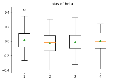
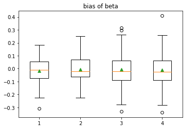
CaseI: The number of samples is N=400.

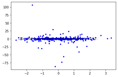
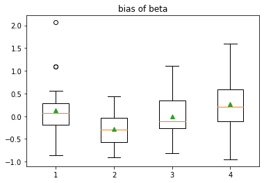
Figure 1 shows the simulation data in CaseI. We replicate this experiment 50 times, and the comparison of different methods are shown in Figure 2 and Table 1.

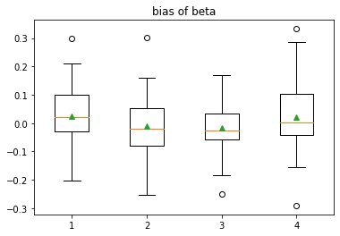
CaseII: The number of samples is N=400.

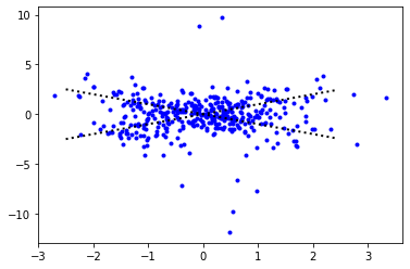
Figure 3 shows the simulation data in CaseII. We replicate this experiment 50 times, and the comparison of different methods are shown in Figure 4 and Table 2.

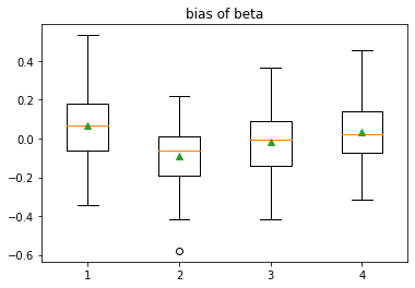
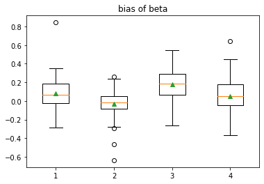
CaseIII: The number of samples is N=400.

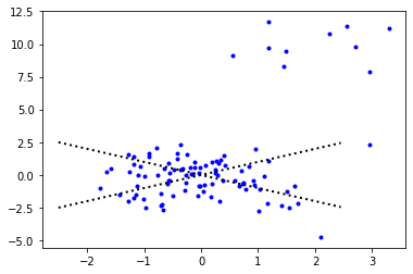
Figure 5 shows the simulation data in CaseIII. We replicate this experiment 50 times, and the comparison of different methods are shown in Figure 6 and Table 3.

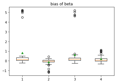
CaseIV: The number of samples is N=400.

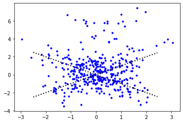
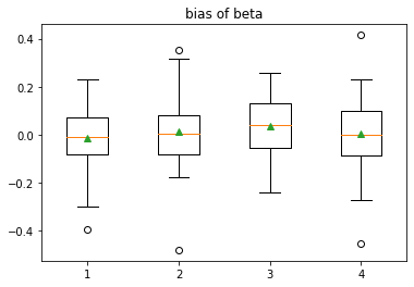
Figure 7 shows the simulation data in CaseIV. We replicate this experiment 50 times, and the comparison of different methods are shown in Figure 8 and Table 4.

It’s hard to choose the dimension of freedom for Mixture of t-distribution. In the experiments shown above, the freedom leading to best results are used. However, the freedom selected by BIC could lead to bad results. In addition, selecting the number of components is also a problem for Mixture regression with t-distribution.

The adaptively trimmed version of MIXT worked well when there are high leverage outliers, but it can deal with drift. We can’t select a proper dimension of freedom for MIXT using BIC when faced with drift.

Adaptively removing abnormal points can improve the estimation accuracy in MixEP. It’s a natural idea is to build a model to cover the drift. This will be the future work.

References

- [1] Huang, T., Peng, H., Zhang, K. (2017). MODEL SELECTION FORGAUSSIAN MIXTURE MODELS. Statistica Sinica, 27(1), 147-169. Re-trieved November 4, 2020, from
- [2] Lange, K. (2016). MM optimization algorithms. Society for Industrial and Applied Mathematics. Weixing Song, Weixin Yao, Yanru Xing,
- [3] Robust mixture regression model fitting by Laplace distribution, Computational Statistics and Data Analysis, Volume 71, 2014, Pages 128-137, ISSN 0167-9473, https://doi.org/10.1016/j.csda.2013.06.022.
- [4] Weixin Yao, Yan Wei, Chun Yu, Robust mixture regression using the t-distribution, Computational Statistics and Data Analysis, Volume 71, 2014, Pages 116-127, ISSN 0167-9473, https://doi.org/10.1016/j.csda.2013.07.019.
- [5] N. Neykov, P. Filzmoser, R. Dimova, P. Neytchev, Robust fitting of mixtures using the trimmed likelihood estimator, Computational Statistics and Data Analysis, Volume 52, Issue 1, 2007, Pages 299-308, ISSN 0167-9473, https://doi.org/10.1016/j.csda.2006.12.024.
- [6] Wennan Chang and Xinyu Zhou and Yong Zang and Chi Zhang and Sha Cao,A New Algorithm using Component-wise Adaptive Trimming For Robust Mixture Regression, 2020. https://arxiv.org/abs/2005.11599
- [7] X. Cao, Q. Zhao, D. Meng, Y. Chen and Z. Xu, Robust Low-Rank Matrix Factorization Under General Mixture Noise Distributions, IEEE Transactions on Image Processing, vol. 25, no. 10, pp. 4677-4690, Oct. 2016, doi: 10.1109/TIP.2016.2593343.
- [8] Liang F, Liu C, Wang N: A robust sequential Bayesian method for identification of differentially expressed genes. Statistica Sinica 17: 571–597. 2007
- [9] Salazar E, Ferreira MAR, Migon HS: Objective Bayesian analysis for exponential power regression models. Sankhya - Series B 74: 107–125. 2012 Ferreira, M.A., Salazar, E. Bayesian reference analysis for exponential power regression models. J Stat Distrib App 1, 12 (2014).