appReferences
Robust Unsupervised Multi-task and Transfer Learning on Gaussian Mixture Models
Abstract
Unsupervised learning has been widely used in many real-world applications. One of the simplest and most important unsupervised learning models is the Gaussian mixture model (GMM). In this work, we study the multi-task learning problem on GMMs, which aims to leverage potentially similar GMM parameter structures among tasks to obtain improved learning performance compared to single-task learning. We propose a multi-task GMM learning procedure based on the EM algorithm that effectively utilizes unknown similarities between related tasks and is robust against a fraction of outlier tasks from arbitrary distributions. The proposed procedure is shown to achieve the minimax optimal rate of convergence for both parameter estimation error and the excess mis-clustering error, in a wide range of regimes. Moreover, we generalize our approach to tackle the problem of transfer learning for GMMs, where similar theoretical results are derived. Additionally, iterative unsupervised multi-task and transfer learning methods may suffer from an initialization alignment problem, and two alignment algorithms are proposed to resolve the issue. Finally, we demonstrate the effectiveness of our methods through simulations and real data examples. To the best of our knowledge, this is the first work studying multi-task and transfer learning on GMMs with theoretical guarantees.
Keywords: Multi-task learning, transfer learning, unsupervised learning, Gaussian mixture models, robustness, minimax rate, EM algorithm
1 Introduction
1.1 Gaussian mixture models (GMMs)
Unsupervised learning that learns patterns from unlabeled data is a prevalent problem in statistics and machine learning. Clustering is one of the most important problems in unsupervised learning, where the goal is to group the observations based on some metrics of similarity. Researchers have developed numerous clustering methods including -means (Forgy, , 1965), -medians (Jain and Dubes, , 1988), spectral clustering (Ng et al., , 2001), and hierarchical clustering (Murtagh and Contreras, , 2012), among others. On the other hand, clustering problems have been analyzed from the perspective of the mixture of several probability distributions (Scott and Symons, , 1971). The mixture of Gaussian distributions is one of the simplest models in this category and has been widely applied in many real applications (Yang and Ahuja, , 1998; Lee et al., , 2012).
In the binary Gaussian mixture models (GMMs) with common covariances, each observation comes from the following mixture of two Gaussian distributions:
| (1) | ||||
| (2) |
where , , and are parameters. This is the same setting as the linear discriminant analysis (LDA) problem in classification (Hastie et al., , 2009), except that the label is unknown in the clustering problem, while it is observed in the classification case. It has been shown that the Bayes classifier for the LDA problem is
| (3) |
where and . Note that is usually referred to as the discriminant coefficient (Anderson, , 1958; Efron, , 1975). Naturally, this classifier is useful in clustering too. In clustering, after learning , , and , we can plug their estimators into (3) to group any new observation . Generally, we define the mis-clustering error rate of any given clustering method as
| (4) |
where is a permutation function, is the label of a future observation , and the probability is taken w.r.t. the joint distribution of based on parameters , , and . Here the error is calculated up to a permutation due to the lack of label information. It is clear that in the ideal case where the parameters are known, in (3) achieves the optimal mis-clustering error. Multi-cluster Gaussian mixture models with components can be described in a similar way. We provide the details in Section S.1 of the supplementary materials.
There is a large volume of published studies on learning a GMM. The vast majority of approaches can be roughly divided into three categories. The first category is the method of moments, where the parameters are estimated through several moment equations (Pearson, , 1894; Kalai et al., , 2010; Hsu and Kakade, , 2013; Ge et al., , 2015). The second category is the spectral method, where the estimation is based on the spectral decomposition (Vempala and Wang, , 2004; Hsu and Kakade, , 2013; Jin et al., , 2017). The last category is the likelihood-based method including the popular expectation-maximization (EM) algorithm as a canonical example. The general form of the EM algorithm was formalized by Dempster et al., (1977) in the context of incomplete data, though earlier works (Hartley, , 1958; Hasselblad, , 1966; Baum et al., , 1970; Sundberg, , 1974) have studied EM-style algorithms in various concrete settings. Classical convergence results on the EM algorithm (Wu, , 1983; Redner and Walker, , 1984; Meng and Rubin, , 1994; McLachlan and Krishnan, , 2007) guarantee local convergence of the algorithm to fixed points of the sample likelihood. Recent advances in the analysis of EM algorithm and its variants provide stronger guarantees by establishing geometric convergence rates of the algorithm to the underlying true parameters under mild initialization conditions. See, for example, Dasgupta and Schulman, (2013); Wang et al., (2014); Xu et al., (2016); Balakrishnan et al., (2017); Yan et al., (2017); Cai et al., (2019); Kwon and Caramanis, (2020); Zhao et al., (2020) for GMM related works. In this paper, we propose modified versions of the EM algorithm with similarly strong guarantees to learn GMMs, under the new context of multi-task and transfer learning.
1.2 Multi-task learning and transfer learning
Multi-tasking is an ability that helps people pay attention to more than one task simultaneously. Moreover, we often find that the knowledge learned from one task can also be useful in other tasks. Multi-task learning (MTL) is a learning paradigm inspired by the human learning ability, which aims to learn multiple tasks and improve performance by utilizing the similarity between these tasks (Zhang and Yang, , 2021). There has been numerous research on MTL, which can be classified into five categories (Zhang and Yang, , 2021): feature learning approach (Argyriou et al., , 2008; Obozinski et al., , 2006), low-rank approach (Ando et al., , 2005), task clustering approach (Thrun and O’Sullivan, , 1996), task relation learning approach (Evgeniou and Pontil, , 2004) and decomposition approach (Jalali et al., , 2010). The majority of existing works focus on the use of MTL in supervised learning problems, while the application of MTL in unsupervised learning, such as clustering, has received less attention. Zhang and Zhang, (2011) developed an MTL clustering method based on a penalization framework, where the objective function consists of a local loss function and a pairwise task regularization term, both of which are related to the Bregman divergence. In Gu et al., (2011), a reproducing kernel Hilbert space (RKHS) was first established, and then a multi-task kernel k-means clustering was applied based on that RKHS. Yang et al., (2014) proposed a spectral MTL clustering method with a novel -norm, which can also produce a linear regression function to predict labels for out-of-sample data. Zhang et al., (2018) suggested a new method based on the similarity matrix of samples in each task, which can learn the within-task clustering structure as well as the task relatedness simultaneously. Marfoq et al., (2021) established a new federated multi-task EM algorithm to learn the mixture of distributions and provided some theory on the convergence guarantee, but the statistical properties of the estimators were not fully understood. Zhang and Chen, (2022) proposed a distributed learning algorithm for GMMs based on transportation divergence when all GMMs are identical. In general, there are very few theoretical results about unsupervised MTL.
Transfer learning (TL) is another learning paradigm similar to multi-task learning but has different objectives. While MTL aims to learn all the tasks well with no priority for any specific task, the goal of TL is to improve the performance on the target task using the information from the source tasks (Zhang and Yang, , 2021). According to Pan and Yang, (2009), most of TL approaches can be classified into four categories: instance-based transfer (Dai et al., , 2007), feature representation transfer (Dai et al., , 2008), parameter transfer (Lawrence and Platt, , 2004) and relational-knowledge transfer (Mihalkova et al., , 2007). Similar to MTL, most of the TL methods focus on supervised learning. Some TL approaches are also developed for the semi-supervised learning setting (Chattopadhyay et al., , 2012; Li et al., , 2013), where only part of target or source data is labeled. There are much fewer discussions on the unsupervised TL approaches 111There are different definitions for unsupervised TL. Sometimes people call the semi-supervised TL an unsupervised TL as well. We follow the definition in Pan and Yang, (2009) here., which focuses on the cases where both target and source data are unlabeled. Dai et al., (2008) developed a co-clustering approach to transfer information from a single source to the target, which relies on the loss in mutual information and requires the features to be discrete. Wang et al., (2008) proposed a TL discriminant analysis method, where the target data is allowed to be unlabeled, but some labeled source data is necessary. In Wang et al., (2021), a TL approach was developed to learn Gaussian mixture models with only one source by weighting the target and source likelihood functions. Zuo et al., (2018) proposed a TL method based on infinite Gaussian mixture models and active learning, but their approach needs sufficient labeled source data and a few labeled target samples.
There are some recent studies on TL and MTL under various statistical settings, including high-dimensional linear regression (Xu and Bastani, , 2021; Li et al., 2022b, ; Zhang et al., , 2022; Li et al., 2022a, ), high-dimensional generalized linear models (Bastani, , 2021; Li et al., , 2023; Tian and Feng, , 2023), functional linear regression (Lin and Reimherr, , 2022), high-dimensional graphical models (Li et al., 2022b, ), reinforcement learning (Chen et al., , 2022), among others. The recent work Duan and Wang, (2023) developed an adaptive and robust MTL framework with sharp statistical guarantees for a broad class of models. We discuss its connection to our work in Section 2.
1.3 Our contributions and paper structure
Our main contributions in this work can be summarized in the following:
-
(i)
We develop efficient polynomial-time iterative procedures to learn GMMs in both MTL and TL settings. These procedures can be viewed as adaptations of the standard EM algorithm for MTL and TL problems.
-
(ii)
The developed procedures come with provable statistical guarantees. Specifically, we derive the upper bounds of their estimation and excess mis-clustering error rates under mild conditions. For MTL, it is shown that when the tasks are close to each other, our method can achieve better upper bounds than those from the single-task learning; when the tasks are substantially different from each other, our method can still obtain competitive convergence rates compared to single-task learning. Similarly for TL, our method can achieve better upper bounds than those from fitting GMM only to target data when the target and sources are similar, and remains competitive otherwise. In addition, the derived upper bounds reveal the robustness of our methods against a fraction of outlier tasks (for MTL) or outlier sources (for TL) from arbitrary distributions. These guarantees certify our procedures as adaptive (to the unknown task relatedness) and robust (to contaminated data) learning approaches.
-
(iii)
We derive the minimax lower bounds for parameter estimation and excess mis-clustering errors. In various regimes, the upper bounds from our methods match the lower bounds (up to small order terms), showing that the proposed methods are (nearly) minimax rate optimal.
-
(iv)
Our MTL and TL approaches require the initial estimates for different tasks to be “well-aligned”, due to the non-identifiability of GMM. We propose two pre-processing alignment algorithms to provably resolve the alignment problem. Similar problems arise in many unsupervised MTL settings. However, to our knowledge, there is no formal discussion of the alignment issue in the existing literature on unsupervised MTL (Gu et al., , 2011; Zhang and Zhang, , 2011; Yang et al., , 2014; Zhang et al., , 2018; Dieuleveut et al., , 2021; Marfoq et al., , 2021). Therefore, our rigorous treatment of the alignment problem is an important step forward in this field.
The rest of the paper is organized as follows. In Section 2, we first discuss the multi-task learning problem for binary GMMs, by introducing the problem setting, our method, and the associated theory. The above-mentioned alignment problem is discussed in Section 2.4. We present a simulation study in Section 3 to validate our theory. Finally, in Section 4, we point out some interesting future research directions. Due to the space limit, the extension to multi-cluster GMMs, additional numerical results, a full treatment of the transfer learning problem, and all the proofs are delegated to the supplementary materials.
We summarize the notations used throughout the paper here for convenience. We use bold capital letters (e.g., ) to denote matrices and use bold small letters (e.g., , ) to denote vectors. For a matrix , its 2-norm or spectral norm is defined as . If , becomes a -dimensional vector and equals its Euclidean norm. For symmetric , we define and as the maximum and minimum eigenvalues of , respectively. For two non-zero real sequences and , we use , or to represent as . And , or means . For two random variable sequences and , the notation means that for any , there exists a positive constant such that . For two real numbers and , and represent and , respectively. For any positive integer , both and stand for the set . For any set , denotes its cardinality, and denotes its complement. Without further notice, , , , , represent some positive constants and can change from line to line.
2 Multi-task Learning
2.1 Problem setting
Suppose there are tasks, for which we have observations from the -th task. Suppose there exists an unknown subset , such that observations from each task in independently follow a GMM, while samples from tasks outside can be arbitrarily distributed. This means,
| (5) |
for all , , and
| (6) |
where is some probability measure on and . In unsupervised learning, we have no access to the true labels . To formalize the multi-task learning problem, we first introduce the parameter space for a single GMM:
| (7) | ||||
| (8) |
where , and are some fixed positive constants. For simplicity, throughout the main text, we assume these constants are fixed. Hence, we have suppressed the dependency on them in the notation . The parameter space is a standard formulation. Similar parameter spaces have been considered, for example, in Cai et al., (2019).
Our goal of multi-task learning is to leverage the potential similarity shared by different tasks in to collectively learn them all. The tasks outside can be arbitrarily distributed and they can be potentially outlier tasks. This motivates us to define a joint parameter space for GMMs in :
| (9) |
where is called the discriminant coefficient in the -th task (recall Section 1.1). For convenience, we define , which together with is part of the decision boundary. Note that this parameter space is defined only for GMMs of tasks in . To model potentially corrupted or contaminated data, we do not impose any distributional constraints for tasks in . Such a modeling framework is reminiscent of Huber’s -contamination model (Huber, , 1964). Similar formulations have been adopted in recent multi-task learning research such as Konstantinov et al., (2020) and Duan and Wang, (2023).
For GMMs in , we assume that they share similar discriminant coefficients. The similarity is formalized by assuming that all the discriminant coefficients in are within Euclidean distance from a “center”. Given that the discriminant coefficient has a major impact on the clustering performance (see the discriminant rule in (3)), the parameter space is tailored to characterize the task relatedness from the clustering perspective. A similar viewpoint that focuses on modeling the discriminant coefficient has appeared in the study of high-dimensional GMM clustering (Cai et al., , 2019) and sparse linear discriminant analysis (Cai and Liu, , 2011; Mai et al., , 2012). With both and being unknown in practice, we aim to develop a multi-task learning procedure that is robust to outlier tasks in , and achieves improved performance for tasks in (compared to the single-task learning), in terms of discriminant coefficient estimation and clustering, whenever is small.
The parameter space does not require the mean vectors or the covariance matrices to be similar, although they are not free parameters due to the constraint on . And the mixture proportions do not need to be similar either. We thus avoid imposing restrictive conditions on those parameters. On the other hand, it implies that estimation of the mixture proportions, mean vectors, and covariance matrices in multi-task learning may not be generally improvable over that in the single-task learning. This is verified by the theoretical results in Section 2.3. While the current treatment in the paper does not consider similarity structure among or , our methods and theory can be readily adapted to handle such scenarios, if desired.
There are two main reasons why this MTL problem can be challenging. First, commonly used strategies like data pooling are fragile with respect to outlier tasks and can lead to arbitrarily inaccurate outcomes in the presence of even a small number of outliers. Also, since the distribution of data from outlier tasks can be adversarial to the learner, the idea of outlier task detection in the recent literature (Li et al., , 2021; Tian and Feng, , 2023) may not be applicable. Second, to address the nonconvexity of the likelihood, we propose to explore the similarity among tasks via a generalization of the EM algorithm. However, a clear theoretical understanding of such an iterative procedure requires a delicate analysis of the whole iterative process. In particular, as in the analysis of EM algorithms (Cai et al., , 2019; Kwon and Caramanis, , 2020), the estimates of similar discriminant vectors and other potentially dissimilar parameters are entangled in the iterations. It is highly non-trivial to separate the impact of estimating and other parameters to derive the desired statistical error rates. We manage to address this challenge through a localization technique by carefully shrinking the analysis radius of estimators as the iteration proceeds.
2.2 Method
We aim to tackle the problem of GMM estimation under the context of multi-task learning. The EM algorithm is commonly used to address the non-convexity of the log-likelihood function arising from the latent labels. In the standard EM algorithm, we “classify” the observations (update the posterior) in E-step and update the parameter estimations in M-step (Redner and Walker, , 1984). For multi-task and transfer learning problems, the penalization framework is very popular, where we solve an optimization problem based on a new objective function. This objective function consists of a local loss function and a penalty term, forcing the estimators of similar tasks to be close to each other. For examples, see Zhang and Zhang, (2011); Zhang et al., (2015); Bastani, (2021); Xu and Bastani, (2021); Li et al., (2021); Duan and Wang, (2023); Lin and Reimherr, (2022); Li et al., (2023); Tian and Feng, (2023). Thus motivated, our method seeks a combination of the EM algorithm and the penalization framework.
In particular, we adapt the penalization framework of Duan and Wang, (2023) and modify the updating formulas in the M-step accordingly. The proposed procedure is summarized in Algorithm 1. For simplicity, in Algorithm 1 we have used the notation
| (11) |
Note that is the posterior probability given the observation . The estimated posterior probability is calculated in every E-step given the updated parameter estimates.
Recall that the parameter space introduced in (LABEL:eq:_parameter_space_mtl) does not encode similarity for the mixture proportions , mean vectors , or covariance matrices . Hence, the updates of them in Steps 5-7 are kept the same as in the standard EM algorithm. Regarding the update for discriminant coefficients in Step 9, the quadratic loss function is motivated by the direct estimation of the discriminant coefficient in high-dimensional GMM (Cai et al., , 2019) and high-dimensional LDA literature (Cai and Liu, , 2011; Witten and Tibshirani, , 2011; Fan et al., , 2012; Mai et al., , 2012, 2019). The penalty term in Step 9 penalizes the contrasts of ’s to exploit the similarity structure among tasks. Having the “center” parameter in the penalization induces robustness against outlier tasks. We refer to Duan and Wang, (2023) for a systematic treatment of this penalization framework. It is straightforward to verify that when the tuning parameters are set to zero, Algorithm 1 reduces to the standard EM algorithm performed separately on the tasks. That is, for each , given the parameter estimate from the previous step , we update , , , , and as in Algorithm 1, and update via
| (12) |
For the maximum number of iteration rounds, , our theory will show that is sufficient to reach the desired statistical error rates. In practice, we can terminate the iteration when the change of estimates within two successive rounds falls below some pre-set small tolerance level. We discuss the initialization in detail in Sections 2.3 and 2.4.
2.3 Theory
In this section, we develop statistical theories for our proposed procedure MTL-GMM (see Algorithm 1). As mentioned in Section 2.1, we are interested in the performance of both parameter estimation and clustering, although the latter is the main focus and motivation. First, we impose conditions in the following assumption set.
Assumption 1.
Denote for . The quantity is the Mahalanobis distance between and with covariance matrix , and can be viewed as the signal-to-noise ratio (SNR) in the -th task (Anderson, , 1958). Suppose the following conditions hold:
-
(i)
with a constant ;
-
(ii)
with some constant ;
-
(iii)
Either of the following two conditions holds with some constant :
-
(a)
, ;
-
(b)
, .
-
(a)
-
(iv)
with some constant ;
Remark 1.
These are common and mild conditions related to the sample size, initialization, and signal-to-noise ratio of GMMs. Condition (i) requires the maximum sample size of all tasks not to be much larger than the average sample size of tasks in . Similar conditions can be found in Duan and Wang, (2023). Condition (ii) is the requirement of the sample size of tasks in . The usual condition for low-dimensional single-task learning is (Cai et al., , 2019). The additional term arises from the simultaneous control of performance on all tasks in , where can be as large as . Condition (iii) requires that the initialization should not be too far away from the truth, which is commonly assumed in either the analysis of EM algorithm (Redner and Walker, , 1984; Balakrishnan et al., , 2017; Cai et al., , 2019) or other iterative algorithms like the local estimation used in semi-parametric models (Carroll et al., , 1997; Li and Liang, , 2008) and adaptive Lasso (Zou, , 2006). The two possible forms considered in this condition are due to the fact that binary GMM is only identifiable up to label permutation. Condition (iv) requires that the signal strength of GMM (in terms of Mahalanobis distance) is strong enough, which is usually assumed in the literature about the likelihood-based methods of GMMs (Dasgupta and Schulman, , 2013; Azizyan et al., , 2013; Balakrishnan et al., , 2017; Cai et al., , 2019).
We first establish the rate of convergence for the estimation. Recalling the parameter space in (LABEL:eq:_parameter_space_mtl), let us denote the true parameter by
To better present the results for parameters related to the optimal discriminant rule (3), we further denote
where . Note that is a function of . For the estimators returned by MTL-GMM (see Algorithm 1), we are particularly interested in the following two error metrics:
| (13) | |||
| (14) | |||
| (15) |
where is a permutation on . Again, we take the minimum above because binary GMM is identifiable up to label permutation. The first error metric involves the error for discriminant coefficients and is closely related to the clustering performance. It reveals how well our method utilizes similarity structure in multi-task learning. The second error metric is about the mean vectors and covariance matrix. As discussed in Section 2.1, we shall not expect it to be improved compared to that in single-task learning, as these parameters are not necessarily similar.
We are ready to present upper bounds for the estimation error of MTL-GMM. We recall that and are the parameter space and probability measure that we use in Section 2.1 to describe the data distributions for tasks in and , respectively.
Theorem 1.
(Upper bounds of the estimation error of GMM parameters for MTL-GMM) Suppose Assumption 1 holds for some with and . Let , and with some constants 222 and depend on the constants , , and etc.. Then there exist a constant , such that for any and any probability measure on , with probability , the following hold for all :
| (16) |
| (17) |
where is some constant and . When with a large constant , the last term on the right-hand side will be dominated by other terms in both inequalities.
The upper bound of contains two parts. The first part is comparable to the single-task learning rate (Cai et al., , 2019) (up to a term due to the simultaneous control over all tasks in ), and the second part characterizes the geometric convergence of iterates. As expected, since , , in are not necessarily similar, an improved error rate over single-task learning is generally impossible. The upper bound for is directly related to the clustering performance of our method. Thus we will provide a detailed discussion about it after presenting the clustering result in the next theorem.
As introduced in Section 1.1, using the estimate from Algorithm 1, we can construct a classifier for task as
| (18) |
Recall that for a clustering method , its mis-clustering error rate under GMM with parameter is
| (19) |
where is a future observation associated with the label , independent from ; the probability is w.r.t. , and the minimum is taken over two permutation functions on . Denote as the Bayes classifier that minimizes . In the following theorem, we obtain the upper bound of the excess mis-clustering error of for .
Theorem 2.
(Upper bound of the excess mis-clustering error for MTL-GMM) Suppose the same conditions in Theorem 1 hold. Then there exist a constant such that for any and any probability measure on , with probability , the following holds for all :
| (20) | ||||
| (21) |
with some . When with a large constant , the last term on the right-hand side will be dominated by the second term.
The upper bounds of in Theorem 1 and in Theorem 2 consist of five parts with one-to-one correspondence. It is sufficient to discuss the bound of . Part (\@slowromancapi@) represents the “oracle rate”, which can be achieved when all tasks in are the same. This is the best rate to possibly achieve. Part (\@slowromancapii@) is a dimension-free error caused by estimating scalar parameters and that appears in the optimal discriminant rule. Part (\@slowromancapiii@) includes that measures the degree of similarity among the tasks in . When these tasks are very similar, will be small, contributing a small term to the upper bound. Nicely, even when is large, the term becomes and it is still comparable to the minimax error rate of single-task learning (e.g., Theorems 4.1 and 4.2 in Cai et al., (2019)). We have the extra term here due to the simultaneous control over all tasks in . Part (\@slowromancapiv@) quantifies the influence from the outlier tasks in . When there are more outlier tasks, increases, and the bound becomes worse. On the other hand, as long as is small enough to make this term dominated by any other part, the error rate induced by outlier tasks becomes negligible. Given that data from outlier tasks can be arbitrarily contaminated, we can conclude that our method is robust against a fraction of outlier tasks from arbitrary sources. The term in Part (\@slowromancapv@) decreases geometrically in the iteration number , implying that the iterates in Algorithm 1 converge geometrically to a ball of radius determined by the errors from Parts (\@slowromancapi@)-(\@slowromancapiv@).
After explaining each part of the upper bound, we now compare it with the convergence rate (including here since we consider all the tasks simultaneously) in the single-task learning and reveal how our method performs. With a quick inspection, we can conclude the following:
-
•
The rate of the upper bound is never larger than . So, in terms of rate of convergence, our method MTL-GMM performs at least as well as single-task learning, regardless of the similarity level and outlier task fraction .
-
•
When (large total sample size for tasks in ), increases with (diverging dimension), (sufficient similarity between tasks in ), and (small fraction of outlier tasks), MTL-GMM attains a faster excess mis-clustering error rate and improves over single-task learning.
The preceding discussions on the upper bounds have demonstrated the superiority of our method. But can we do better? To further evaluate the upper bounds of our method, we next derive complementary minimax lower bounds for both estimation error and excess mis-clustering error. We will show that our method is (nearly) minimax rate optimal in a broad range of regimes.
Theorem 3.
(Lower bounds of the estimation error of GMM parameters in multi-task learning) Suppose . Suppose there exists a subset with such that and , where are some constants. Then
| (22) | ||||
| (23) |
| (24) | ||||
| (25) |
Theorem 4.
(Lower bound of the excess mis-clustering error in multi-task learning) Suppose the same conditions in Theorem 3 hold. Then
| (26) | ||||
| (27) |
Comparing the upper and lower bounds in Theorems 1-4, we make several remarks:
-
•
Regarding the estimation of mean vectors and covariance matrices , the upper and lower bounds match, hence our method is minimax rate optimal.
-
•
For the estimation error and excess mis-clustering error with , the first three terms in the upper and lower bounds match. Only the term involving in the lower bound differs from that in the upper bound by a factor or . As a result, in the classical low-dimensional regime where is bounded, the upper and lower bounds match (up to a logarithmic factor). Therefore, our method is (nearly) minimax rate optimal for estimating and clustering in such a classical regime.
-
•
When the dimension diverges, there might exist a non-negligible gap between the upper and lower bounds for and with . Nevertheless, this only occurs when the fraction of outlier task is above the threshold . Below the threshold, our method remains minimax rate optimal even though is unbounded.
-
•
Does the gap, when it exists, arise from the upper bound or the lower bound? We believe that it is the upper bound that sometimes becomes not sharp. As can be seen from the proof of Theorem 1, the term is due to the estimation of those “center” parameters in Algorithm 1. Recent advances in robust statistics (Chen et al., , 2018) have shown that estimators based on statistical depth functions such as Tukey’s depth function (Tukey, , 1975) can achieve optimal minimax rate under Huber’s -contamination model for location and covariance estimation. It might be possible to utilize depth functions to estimate “center” parameters in our problem and kill the factor in the upper bound. We leave a rigorous development of optimal robustness as an interesting future research. On the other hand, such statistical improvement may come with expensive computation, as depth function-based estimation typically requires solving a challenging non-convex optimization problem.
2.4 Initialization and cluster alignment
As specified by Condition (iii) in Assumption 1, our proposed learning procedure requires that for each task in , initial values of the GMM parameter estimates lie within a distance of SNR-order from the ground truth. This can be satisfied by the method of moments proposed in Ge et al., (2015). In practice, a natural initialization method is to run the standard EM algorithm or other common clustering methods like -means on each task and use the corresponding estimate as the initial values. We adopted the standard EM algorithm in our numerical experiments, and the numerical results in Section 3 and supplements showed that this practical initialization works quite well. However, in the context of multi-task learning, Condition (iii) further requires a correct alignment of those good initializations from each task, owing to the non-identifiability of GMMs. We discuss in detail the alignment issue in Section 2.4.1 and propose two algorithms to resolve this issue in Section 2.4.2.
2.4.1 The alignment issue
Recall that Section 2.1 introduces the binary GMM with parameters for each task . Because the two sets of parameter values for index the same distribution, a good initialization close to the truth is up to a permutation of the two cluster labels. The permutations in the initialization of different tasks could be different. Therefore, in light of the joint parameter space defined in (LABEL:eq:_parameter_space_mtl) and Condition (iii) in Assumption 1, for given initializations from different tasks, we may need to permute their cluster labels to feed the well-aligned initialization into Algorithm 1.
We further elaborate on the alignment issue using Algorithm 1. The penalization in Step 9 aims to push the estimators ’s with different towards each other, which is expected to improve the performance thanks to the similarity among underlying true parameters . However, due to the potential permutation of two cluster labels, the vanilla single-task initializations (without alignment) cannot guarantee that the estimators at each iteration are all estimating the corresponding ’s (some may estimate ’s).
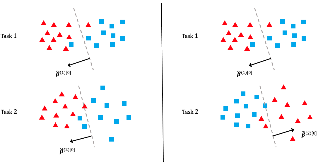
Figure 1 illustrates the alignment issue in the case of two tasks. The left-hand-side situation is ideal where , are estimates of , (which are similar). The right-hand-side situation is problematic because , are estimates of , (which are not similar). Therefore, in practice, after obtaining the initializations from each task, it is necessary to align their cluster labels to ensure that estimators of similar parameters are correctly put together in the penalization framework in Algorithm 1. We formalize the problem and provide two solutions in the next subsection.
2.4.2 Two alignment algorithms
Suppose are the initial estimates of discriminant coefficients with potentially bad alignment for . Note that a good initialization and alignment is not required (in fact, it is not even well defined) for the outlier tasks in , because they can be from arbitrary distributions. However, since is unknown, we will have to address the alignment issue for tasks in based on initial estimates from all the tasks. For binary GMMs, each alignment of can be represented by a -dimensional Rademacher vector . Define the ideal alignment as . The goal is to recover the well-aligned initializers from the initial estimates (equivalently, to recover ), which can then be fed into Algorithm 1. Once are well aligned, other initial estimates in Algorithm 1 will be automatically well aligned.
In the following, we will introduce two alignment algorithms. The first one is the “exhaustive search” method (Algorithm 2), where we search among all possible alignments to find the best one. The second one is the “greedy search” method (Algorithm 3), where we flip the sign of in a greedy way to recover . Both methods are proved to recover under mild conditions. The conditions required by the “exhaustive search” method are slightly weaker than those required by the “greedy search” method. As for computational complexity, the latter enjoys a linear time complexity , while the former suffers from an exponential time complexity due to optimization over all possible alignments.
To this end, for a given alignment with the correspondingly aligned estimates , define its alignment score as
| (28) |
The intuition is that as long as the initializations are close to the ground truth, a smaller score indicates less difference among , which implies a better alignment. The score can be thus used to evaluate the quality of an alignment. Note that the score is defined in a symmetric way, that is, . The exhaustive search algorithm is presented in Algorithm 2, where scores of all alignments are calculated, and the alignment that minimizes the score is output. Since the score is symmetric, there are at least two alignments with the minimum score. The algorithm can arbitrarily choose and output one of them.
The following theorem reveals that the exhaustive search algorithm can successfully find the ideal alignment under mild conditions.
Theorem 5 (Alignment correctness for Algorithm 2).
Remark 2.
The conditions imposed in Theorem 5 are no stronger than conditions required by Theorem 1. First of all, Condition (i) is also required in Theorem 1. Moreover, from the definition of in (LABEL:eq:_parameter_space_mtl), it is bounded by a constant. This together with Conditions (iii) and (iv) in Assumption 1 implies Condition (ii) in Theorem 5.
Remark 3.
With Theorem 5, we can relax the original Condition (iii) in Assumption 1 to the following condition:
For all , either of the following two conditions holds with a sufficiently small constant :
-
(a)
, ;
-
(b)
, .
In the relaxed version, the initialization for each task only needs to be good up to an arbitrary permutation, while in the original version, the initialization for each task needs to be good under the same permutation.
Next, we would like to introduce the second alignment algorithm, the “greedy search” method, summarized in Algorithm 3. The main idea is to flip the sign of the discriminant coefficient estimates (equivalently, swap the two cluster labels) from tasks in a sequential fashion to check whether the alignment score decreases or not. If yes, we keep the alignment after the flip and proceed with the next task. Otherwise, we keep the alignment before the flip and proceed with the next task. A surprising fact of Algorithm 3 is that it is sufficient to iterate this procedure for all tasks just once to recover the ideal alignment, making the algorithm computationally efficient.
To help state the theory of the greedy search algorithm, we define the “mismatch proportion” of as
| (30) |
Intuitively, represents the level of mismatch between the initial alignment and the ideal one. It’s straightforward to verify that ; means the initial alignment equals the ideal one, while (or when is odd) represents the “worst” alignment, where almost half of the tasks are badly-aligned. The smaller is, the better alignment is. Note that we only care about the alignment of tasks in .
The following theorem shows that the greedy search algorithm can succeed in finding the ideal alignment under mild conditions.
Theorem 6 (Alignment correctness for Algorithm 3).
Remark 4.
Conditions (i) and (ii) required by Theorem 6 are similar to the requirements in Theorem 5, which have been shown to be no stronger than conditions in Assumption 1 and Theorem 1 (See Remark 2). However, Condition (iii) is an additional requirement for the success of the greedy label-swapping algorithm. The intuition is that in the exhaustive search algorithm, we compare the scores of all alignments and only need to ensure the ideal alignment can defeat the badly-aligned ones in terms of the alignment score. In contrast, the success of the greedy search algorithm relies on the correct move at each step. We need to guarantee that the “better” alignment after the swap (which may still be badly aligned) can outperform the “worse” one before the swap. This is more difficult to satisfy. Hence, more conditions are needed for the success of Algorithm 3. Condition (iii) is one such condition to provide a reasonably good initial alignment to start the greedy search process. More details of the analysis can be found in the proofs of Theorems 5 and 6 in the supplements.
Remark 5.
In practice, Condition (iii) can fail to hold with a non-zero probability. One solution is to start with random alignments, run the greedy search algorithm multiple times, and use the alignment that appears most frequently in the output. Nevertheless, this will increase the computational burden. In our numerical studies, Algorithm 3 without multiple random alignments works well.
One appealing feature of the two alignment algorithms is that they are robust against a fraction of outlier tasks from arbitrary distributions. According to the definition of the alignment score, this may appear impossible at first glance because the score depends on the estimators from all tasks. However, it turns out that the impact of outliers when comparing the scores in Algorithm 2 and 3 can be bounded by parameters and constants that are unrelated to outlier tasks via the triangle inequality of Euclidean norms. The key idea is that the alignment of outlier tasks in does not matter in Theorems 5 and 6. More details can be found in the proof of Theorems 5 and 6 in the supplementary materials.
In contrast with supervised MTL, the alignment issue commonly exists in unsupervised MTL. It generally occurs when aggregating information (up to latent label permutation) across different tasks. Alignment pre-processing is thus necessary and important. However, to our knowledge, there is no formal discussion regarding alignment in the existing literature of unsupervised MTL (Gu et al., , 2011; Zhang and Zhang, , 2011; Yang et al., , 2014; Zhang et al., , 2018; Dieuleveut et al., , 2021; Marfoq et al., , 2021). Our treatment of alignment in Section 2.4 is an important step forward in this field. Our algorithms can be potentially extended to other unsupervised MTL scenarios and we leave it for future studies.
3 Simulations
In this section, we present a simulation study of our multi-task learning procedure MTL-GMM, i.e., Algorithms 1. The tuning parameter is set as , and the value of is determined by a 10-fold cross-validation based on the log-likelihood of the final fitted model. The candidates of are chosen in a data-driven way, which is described in detail in Section S.3.1.5 of the supplements. All the experiments in this section are implemented in R. Function Mcluster in R package mclust is called to fit a single GMM. We also conducted two additional simulation studies and two real-data studies. Due to the page limit, we included these in Section S.3 of the supplementary materials.
We consider a binary GMM setting. There are tasks of which each has sample size and dimension . When , we generate each from and from , where , , and let . When , the distributions still follow GMM, but we generate each from and from , and let , . In this setup, it is clear that quantifies the similarity among tasks in , and tasks in have very distinct distributions and can be viewed as outlier tasks. For a given , the outlier task index set in each replication is uniformly sampled from all subsets of with cardinality . We consider two cases:
-
(i)
No outlier tasks (), and changes from 0 to 10 with increment 1;
-
(ii)
2 outlier tasks (), and changes from 0 to 10 with increment 1;
We fit Single-task-GMM on each separate task, Pooled-GMM on the merged data of all tasks, and our MTL-GMM in Algorithm 1 coupled with the exhaustive search for the alignment in Algorithm 2. The performances of all three methods are evaluated by the estimation error of , , , , , and , as well as the empirical mis-clustering error calculated on a test data set of size 500, for tasks in . Due to page limit, we only present the estimation error of and the mis-clustering error here, and leave the others to Section S.3.1.1 of the supplements. These two errors are the maximum errors over tasks in . For each setting, the simulation is replicated 200 times, and the average of the maximum errors together with the standard deviation are reported in Figure 2.
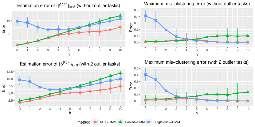
When there are no outlier tasks, it can be seen that MTL-GMM and Pooled-GMM are competitive when is small (i.e. the tasks are similar), and they outperform Single-task-GMM. As increases (i.e. tasks become more heterogenous), MTL-GMM starts to outperform Pooled-GMM by a large margin. Moreover, MTL-GMM is significantly better than Single-task-GMM in terms of both estimation and mis-clustering errors over a wide range of . These comparisons demonstrate that MTL-GMM not only effectively utilizes the unknown similarity structure among tasks, but also adapts to it. When the outlier tasks exist, even when is very small, MTL-GMM still performs better than Pooled-GMM, showing the robustness of MTL-GMM against a fraction of outlier tasks.
4 Discussions
We would like to highlight several interesting open problems for potential future work:
-
•
What if only some clusters are similar among different tasks? This may be a more realistic situation in particular when there are more than 2 clusters in each task. Our current proposed algorithms may not work well because they do not take into account this extra layer of heterogeneity. Furthermore, in this situation, different tasks may have a different number of Gaussian clusters. Such a setting with various numbers of clusters has been considered in some literature on general unsupervised multi-task learning (Zhang and Zhang, , 2011; Yang et al., , 2014; Zhang et al., , 2018). It would be of great interest to develop multi-task and transfer learning methods with provable guarantees for GMMs under these more complicated settings.
-
•
How to accommodate heterogeneous covariance matrices for different Gaussian clusters within each task? This is related to the quadratic discriminant analysis (QDA) in supervised learning where the Bayes classifier has a leading quadratic term. It may require more delicate analysis for methodological and theoretical development. Some recent QDA literature might be helpful (Li and Shao, , 2015; Fan et al., , 2015; Hao et al., , 2018; Jiang et al., , 2018).
-
•
In this paper, we have focused on the pure unsupervised learning problem, where all the samples are unlabeled. It would be interesting to consider the semi-supervised learning setting, where labels in some tasks (or sources) are known. Li et al., 2022a discusses a similar problem under the linear regression setting, but how the labeled data can help the estimation and clustering in the context of GMMs remains unknown.
References
- Anderson, (1958) Anderson, T. W. (1958). An introduction to multivariate statistical analysis: Wiley series in probability and mathematical statistics: Probability and mathematical statistics.
- Ando et al., (2005) Ando, R. K., Zhang, T., and Bartlett, P. (2005). A framework for learning predictive structures from multiple tasks and unlabeled data. Journal of Machine Learning Research, 6(11).
- Argyriou et al., (2008) Argyriou, A., Evgeniou, T., and Pontil, M. (2008). Convex multi-task feature learning. Machine learning, 73(3):243–272.
- Azizyan et al., (2013) Azizyan, M., Singh, A., and Wasserman, L. (2013). Minimax theory for high-dimensional gaussian mixtures with sparse mean separation. Advances in Neural Information Processing Systems, 26.
- Balakrishnan et al., (2017) Balakrishnan, S., Wainwright, M. J., and Yu, B. (2017). Statistical guarantees for the em algorithm: From population to sample-based analysis. The Annals of Statistics, 45(1):77–120.
- Bastani, (2021) Bastani, H. (2021). Predicting with proxies: Transfer learning in high dimension. Management Science, 67(5):2964–2984.
- Baum et al., (1970) Baum, L. E., Petrie, T., Soules, G., and Weiss, N. (1970). A maximization technique occurring in the statistical analysis of probabilistic functions of markov chains. The Annals of Mathematical Statistics, 41(1):164–171.
- Cai and Liu, (2011) Cai, T. and Liu, W. (2011). A direct estimation approach to sparse linear discriminant analysis. Journal of the American statistical association, 106(496):1566–1577.
- Cai et al., (2019) Cai, T. T., Ma, J., and Zhang, L. (2019). Chime: Clustering of high-dimensional gaussian mixtures with em algorithm and its optimality. The Annals of Statistics, 47(3):1234–1267.
- Carroll et al., (1997) Carroll, R. J., Fan, J., Gijbels, I., and Wand, M. P. (1997). Generalized partially linear single-index models. Journal of the American Statistical Association, 92(438):477–489.
- Chattopadhyay et al., (2012) Chattopadhyay, R., Sun, Q., Fan, W., Davidson, I., Panchanathan, S., and Ye, J. (2012). Multisource domain adaptation and its application to early detection of fatigue. ACM Transactions on Knowledge Discovery from Data (TKDD), 6(4):1–26.
- Chen et al., (2022) Chen, E. Y., Jordan, M. I., and Li, S. (2022). Transferred q-learning. arXiv preprint arXiv:2202.04709.
- Chen et al., (2018) Chen, M., Gao, C., and Ren, Z. (2018). Robust covariance and scatter matrix estimation under huber’s contamination model. The Annals of Statistics, 46(5):1932–1960.
- Dai et al., (2007) Dai, W., Yang, Q., Xue, G., and Yu, Y. (2007). Boosting for transfer learning. In ACM International Conference Proceeding Series, volume 227, page 193.
- Dai et al., (2008) Dai, W., Yang, Q., Xue, G.-R., and Yu, Y. (2008). Self-taught clustering. In Proceedings of the 25th international conference on Machine learning, pages 200–207.
- Dasgupta and Schulman, (2013) Dasgupta, S. and Schulman, L. (2013). A two-round variant of em for gaussian mixtures. arXiv preprint arXiv:1301.3850.
- Dempster et al., (1977) Dempster, A. P., Laird, N. M., and Rubin, D. B. (1977). Maximum likelihood from incomplete data via the em algorithm. Journal of the Royal Statistical Society: Series B (Methodological), 39(1):1–22.
- Dieuleveut et al., (2021) Dieuleveut, A., Fort, G., Moulines, E., and Robin, G. (2021). Federated-em with heterogeneity mitigation and variance reduction. Advances in Neural Information Processing Systems, 34:29553–29566.
- Duan and Wang, (2023) Duan, Y. and Wang, K. (2023). Adaptive and robust multi-task learning. The Annals of Statistics, 51(5):2015–2039.
- Efron, (1975) Efron, B. (1975). The efficiency of logistic regression compared to normal discriminant analysis. Journal of the American Statistical Association, 70(352):892–898.
- Evgeniou and Pontil, (2004) Evgeniou, T. and Pontil, M. (2004). Regularized multi–task learning. In Proceedings of the tenth ACM SIGKDD international conference on Knowledge discovery and data mining, pages 109–117.
- Fan et al., (2012) Fan, J., Feng, Y., and Tong, X. (2012). A road to classification in high dimensional space: the regularized optimal affine discriminant. Journal of the Royal Statistical Society: Series B (Statistical Methodology), 74(4):745–771.
- Fan et al., (2015) Fan, Y., Kong, Y., Li, D., and Zheng, Z. (2015). Innovated interaction screening for high-dimensional nonlinear classification. The Annals of Statistics, 43(3):1243–1272.
- Forgy, (1965) Forgy, E. W. (1965). Cluster analysis of multivariate data: efficiency versus interpretability of classifications. Biometrics, 21:768–769.
- Ge et al., (2015) Ge, R., Huang, Q., and Kakade, S. M. (2015). Learning mixtures of gaussians in high dimensions. In Proceedings of the forty-seventh annual ACM symposium on Theory of computing, pages 761–770.
- Gu et al., (2011) Gu, Q., Li, Z., and Han, J. (2011). Learning a kernel for multi-task clustering. In Proceedings of the AAAI Conference on Artificial Intelligence, volume 25, pages 368–373.
- Hao et al., (2018) Hao, N., Feng, Y., and Zhang, H. H. (2018). Model selection for high-dimensional quadratic regression via regularization. Journal of the American Statistical Association, 113(522):615–625.
- Hartley, (1958) Hartley, H. O. (1958). Maximum likelihood estimation from incomplete data. Biometrics, 14(2):174–194.
- Hasselblad, (1966) Hasselblad, V. (1966). Estimation of parameters for a mixture of normal distributions. Technometrics, 8(3):431–444.
- Hastie et al., (2009) Hastie, T., Tibshirani, R., Friedman, J. H., and Friedman, J. H. (2009). The elements of statistical learning: data mining, inference, and prediction, volume 2. Springer.
- Hsu and Kakade, (2013) Hsu, D. and Kakade, S. M. (2013). Learning mixtures of spherical gaussians: moment methods and spectral decompositions. In Proceedings of the 4th conference on Innovations in Theoretical Computer Science, pages 11–20.
- Huber, (1964) Huber, P. J. (1964). Robust estimation of a location parameter. The Annals of Mathematical Statistics, pages 73–101.
- Jain and Dubes, (1988) Jain, A. K. and Dubes, R. C. (1988). Algorithms for clustering data. Prentice-Hall, Inc.
- Jalali et al., (2010) Jalali, A., Sanghavi, S., Ruan, C., and Ravikumar, P. (2010). A dirty model for multi-task learning. Advances in neural information processing systems, 23.
- Jiang et al., (2018) Jiang, B., Wang, X., and Leng, C. (2018). A direct approach for sparse quadratic discriminant analysis. Journal of Machine Learning Research, 19(1):1098–1134.
- Jin et al., (2017) Jin, J., Ke, Z. T., and Wang, W. (2017). Phase transitions for high dimensional clustering and related problems. The Annals of Statistics, 45(5):2151–2189.
- Kalai et al., (2010) Kalai, A. T., Moitra, A., and Valiant, G. (2010). Efficiently learning mixtures of two gaussians. In Proceedings of the forty-second ACM symposium on Theory of computing, pages 553–562.
- Konstantinov et al., (2020) Konstantinov, N., Frantar, E., Alistarh, D., and Lampert, C. (2020). On the sample complexity of adversarial multi-source pac learning. In International Conference on Machine Learning, pages 5416–5425. PMLR.
- Kwon and Caramanis, (2020) Kwon, J. and Caramanis, C. (2020). The em algorithm gives sample-optimality for learning mixtures of well-separated gaussians. In Conference on Learning Theory, pages 2425–2487. PMLR.
- Lawrence and Platt, (2004) Lawrence, N. D. and Platt, J. C. (2004). Learning to learn with the informative vector machine. In Proceedings of the twenty-first international conference on Machine learning, page 65.
- Lee et al., (2012) Lee, K., Guillemot, L., Yue, Y., Kramer, M., and Champion, D. (2012). Application of the gaussian mixture model in pulsar astronomy-pulsar classification and candidates ranking for the fermi 2fgl catalogue. Monthly Notices of the Royal Astronomical Society, 424(4):2832–2840.
- Li and Shao, (2015) Li, Q. and Shao, J. (2015). Sparse quadratic discriminant analysis for high dimensional data. Statistica Sinica, pages 457–473.
- Li and Liang, (2008) Li, R. and Liang, H. (2008). Variable selection in semiparametric regression modeling. The Annals of Statistics, 36(1):261–286.
- Li et al., (2023) Li, S., Cai, T., and Duan, R. (2023). Targeting underrepresented populations in precision medicine: A federated transfer learning approach. The Annals of Applied Statistics, 17(4):2970–2992.
- Li et al., (2021) Li, S., Cai, T. T., and Li, H. (2021). Transfer learning for high-dimensional linear regression: Prediction, estimation and minimax optimality. Journal of the Royal Statistical Society: Series B (Statistical Methodology), pages 1–25.
- (46) Li, S., Cai, T. T., and Li, H. (2022a). Estimation and inference with proxy data and its genetic applications. arXiv preprint arXiv:2201.03727.
- (47) Li, S., Cai, T. T., and Li, H. (2022b). Transfer learning in large-scale gaussian graphical models with false discovery rate control. Journal of the American Statistical Association, pages 1–13.
- Li et al., (2013) Li, W., Duan, L., Xu, D., and Tsang, I. W. (2013). Learning with augmented features for supervised and semi-supervised heterogeneous domain adaptation. IEEE transactions on pattern analysis and machine intelligence, 36(6):1134–1148.
- Lin and Reimherr, (2022) Lin, H. and Reimherr, M. (2022). On transfer learning in functional linear regression. arXiv preprint arXiv:2206.04277.
- Mai et al., (2019) Mai, Q., Yang, Y., and Zou, H. (2019). Multiclass sparse discriminant analysis. Statistica Sinica, 29(1):97–111.
- Mai et al., (2012) Mai, Q., Zou, H., and Yuan, M. (2012). A direct approach to sparse discriminant analysis in ultra-high dimensions. Biometrika, 99(1):29–42.
- Marfoq et al., (2021) Marfoq, O., Neglia, G., Bellet, A., Kameni, L., and Vidal, R. (2021). Federated multi-task learning under a mixture of distributions. Advances in Neural Information Processing Systems, 34:15434–15447.
- McLachlan and Krishnan, (2007) McLachlan, G. J. and Krishnan, T. (2007). The EM algorithm and extensions. John Wiley & Sons.
- Meng and Rubin, (1994) Meng, X.-L. and Rubin, D. B. (1994). On the global and componentwise rates of convergence of the em algorithm. Linear Algebra and its Applications, 199:413–425.
- Mihalkova et al., (2007) Mihalkova, L., Huynh, T., and Mooney, R. J. (2007). Mapping and revising markov logic networks for transfer learning. In Proceedings of the 22nd national conference on Artificial intelligence-Volume 1, pages 608–614.
- Murtagh and Contreras, (2012) Murtagh, F. and Contreras, P. (2012). Algorithms for hierarchical clustering: an overview. Wiley Interdisciplinary Reviews: Data Mining and Knowledge Discovery, 2(1):86–97.
- Ng et al., (2001) Ng, A., Jordan, M., and Weiss, Y. (2001). On spectral clustering: Analysis and an algorithm. Advances in neural information processing systems, 14.
- Obozinski et al., (2006) Obozinski, G., Taskar, B., and Jordan, M. (2006). Multi-task feature selection. Statistics Department, UC Berkeley, Tech. Rep, 2(2.2):2.
- Pan and Yang, (2009) Pan, S. J. and Yang, Q. (2009). A survey on transfer learning. IEEE Transactions on knowledge and data engineering, 22(10):1345–1359.
- Pearson, (1894) Pearson, K. (1894). Contributions to the mathematical theory of evolution. Philosophical Transactions of the Royal Society of London. A, 185:71–110.
- Redner and Walker, (1984) Redner, R. A. and Walker, H. F. (1984). Mixture densities, maximum likelihood and the em algorithm. SIAM review, 26(2):195–239.
- Scott and Symons, (1971) Scott, A. J. and Symons, M. J. (1971). Clustering methods based on likelihood ratio criteria. Biometrics, pages 387–397.
- Sundberg, (1974) Sundberg, R. (1974). Maximum likelihood theory for incomplete data from an exponential family. Scandinavian Journal of Statistics, pages 49–58.
- Thrun and O’Sullivan, (1996) Thrun, S. and O’Sullivan, J. (1996). Discovering structure in multiple learning tasks: The tc algorithm. In ICML, volume 96, pages 489–497.
- Tian and Feng, (2023) Tian, Y. and Feng, Y. (2023). Transfer learning under high-dimensional generalized linear models. Journal of the American Statistical Association, 118(544):2684–2697.
- Tukey, (1975) Tukey, J. W. (1975). Mathematics and the picturing of data. In Proceedings of the International Congress of Mathematicians, Vancouver, 1975, volume 2, pages 523–531.
- Vempala and Wang, (2004) Vempala, S. and Wang, G. (2004). A spectral algorithm for learning mixture models. Journal of Computer and System Sciences, 68(4):841–860.
- Wang et al., (2021) Wang, R., Zhou, J., Jiang, H., Han, S., Wang, L., Wang, D., and Chen, Y. (2021). A general transfer learning-based gaussian mixture model for clustering. International Journal of Fuzzy Systems, 23(3):776–793.
- Wang et al., (2014) Wang, Z., Gu, Q., Ning, Y., and Liu, H. (2014). High dimensional expectation-maximization algorithm: Statistical optimization and asymptotic normality. arXiv preprint arXiv:1412.8729.
- Wang et al., (2008) Wang, Z., Song, Y., and Zhang, C. (2008). Transferred dimensionality reduction. In Joint European conference on machine learning and knowledge discovery in databases, pages 550–565. Springer.
- Witten and Tibshirani, (2011) Witten, D. M. and Tibshirani, R. (2011). Penalized classification using fisher’s linear discriminant. Journal of the Royal Statistical Society: Series B (Statistical Methodology), 73(5):753–772.
- Wu, (1983) Wu, C. J. (1983). On the convergence properties of the em algorithm. The Annals of statistics, pages 95–103.
- Xu et al., (2016) Xu, J., Hsu, D. J., and Maleki, A. (2016). Global analysis of expectation maximization for mixtures of two gaussians. Advances in Neural Information Processing Systems, 29.
- Xu and Bastani, (2021) Xu, K. and Bastani, H. (2021). Learning across bandits in high dimension via robust statistics. arXiv preprint arXiv:2112.14233.
- Yan et al., (2017) Yan, B., Yin, M., and Sarkar, P. (2017). Convergence of gradient em on multi-component mixture of gaussians. Advances in Neural Information Processing Systems, 30.
- Yang and Ahuja, (1998) Yang, M.-H. and Ahuja, N. (1998). Gaussian mixture model for human skin color and its applications in image and video databases. In Storage and retrieval for image and video databases VII, volume 3656, pages 458–466. SPIE.
- Yang et al., (2014) Yang, Y., Ma, Z., Yang, Y., Nie, F., and Shen, H. T. (2014). Multitask spectral clustering by exploring intertask correlation. IEEE transactions on cybernetics, 45(5):1083–1094.
- Zhang and Zhang, (2011) Zhang, J. and Zhang, C. (2011). Multitask bregman clustering. Neurocomputing, 74(10):1720–1734.
- Zhang and Chen, (2022) Zhang, Q. and Chen, J. (2022). Distributed learning of finite gaussian mixtures. Journal of Machine Learning Research, 23(99):1–40.
- Zhang et al., (2022) Zhang, X., Blanchet, J., Ghosh, S., and Squillante, M. S. (2022). A class of geometric structures in transfer learning: Minimax bounds and optimality. In International Conference on Artificial Intelligence and Statistics, pages 3794–3820. PMLR.
- Zhang et al., (2015) Zhang, X., Zhang, X., and Liu, H. (2015). Smart multitask bregman clustering and multitask kernel clustering. ACM Transactions on Knowledge Discovery from Data (TKDD), 10(1):1–29.
- Zhang et al., (2018) Zhang, X., Zhang, X., Liu, H., and Luo, J. (2018). Multi-task clustering with model relation learning. In Proceedings of the 27th International Joint Conference on Artificial Intelligence, pages 3132–3140.
- Zhang and Yang, (2021) Zhang, Y. and Yang, Q. (2021). A survey on multi-task learning. IEEE Transactions on Knowledge and Data Engineering.
- Zhao et al., (2020) Zhao, R., Li, Y., and Sun, Y. (2020). Statistical convergence of the em algorithm on gaussian mixture models. Electronic Journal of Statistics, 14:632–660.
- Zou, (2006) Zou, H. (2006). The adaptive lasso and its oracle properties. Journal of the American Statistical Association, 101(476):1418–1429.
- Zuo et al., (2018) Zuo, H., Lu, J., Zhang, G., and Liu, F. (2018). Fuzzy transfer learning using an infinite gaussian mixture model and active learning. IEEE Transactions on Fuzzy Systems, 27(2):291–303.
Supplementary Materials of “Robust Unsupervised Multi-task and Transfer Learning on Gaussian Mixture Models”
S.1 Extension to Multi-cluster GMMs
In the main text, we have discussed the MTL problem for binary GMMs. In this section, we extend our methods and theory to Gaussian mixtures with clusters ().
We first generalize the problem setting introduced in Sections 1.1 and 2.1. There are tasks where we have observations from the -th task. An unknown subset denotes tasks whose samples follow multi-cluster GMMs, and refers to outlier tasks that can have arbitrary distributions. Specifically, for all ,
| (S.1.32) |
with , and
| (S.1.33) |
where is some probability measure on and . We focus on the following joint parameter space
| (S.1.34) |
where is the -th discriminant coefficient in the -th task, and is the parameter space for a single multi-cluster GMM,
| (S.1.35) | ||||
| (S.1.36) |
Note that (S.1.34) and (S.1.36) are natural generalizations of (LABEL:eq:_parameter_space_mtl) and (8), respectively.
Under a multi-cluster GMM with parameter , compared with (3), the optimal discriminant rule now becomes
| (S.1.37) |
where . Once we have the parameter estimators, we plug them into the above rule to obtain the plug-in clustering method. Recall that for a clustering method , its mis-clustering error is
| (S.1.38) |
Here, is an independent future observation associated with the label , the probability is w.r.t. , and the minimum is taken over permutation functions on . Since (S.1.37) is the optimal clustering method that minimizes , the excess mis-clustering error for a given clustering is . The rest of the section aims to extend the EM-stylized multi-task learning procedure and the two alignment algorithms in Section 2 to the general multi-cluster GMM setting, and provide similar statistical guarantees in terms of estimation and excess mis-clustering errors. For simplicity, throughout this section, we assume the number of clusters to be bounded and known. We leave the case of diverging as a future work.
Since both the EM algorithm and the penalization framework work beyond binary GMM, our methodological idea described in Section 2.2 can be directly adapted to extend Algorithm 1 to the multi-cluster case. We summarize the general procedure in Algorithm 4. Like in Algorithm 1, we have adopted the following notation for posterior probability in Algorithm 4,
| (S.1.39) |
where , , and . Specifically, is the posterior probability given the observation , when the true parameter of a multi-cluster GMM satisfies , for .
Having the estimates from Algorithm 4, we can plug them into (S.1.37) to construct the clustering method, denoted by . Equivalently,
| (S.1.40) |
S.1.1 Theory
We need the following assumption before stating the theory.
Assumption 2.
Denote for . Suppose the following conditions hold:
-
(i)
with a constant ;
-
(ii)
with some constant ;
-
(iii)
There exists a permutation such that
-
(a)
, with some constant ;
-
(b)
.
-
(a)
-
(iv)
with some constant ;
Remark 6.
We first present the result for parameter estimation. We adopt similar error metrics as the ones in (14) and (15). Specifically, denote the true parameter by which belongs to the parameter space in (S.1.34). For each , define the functional , where . For the estimators returned by Algorithm 4, we are interested in the error metrics 333Similar to the binary case, the minimum is taken due to the non-identifiability in multi-cluster GMMs.:
| (S.1.41) | |||
| (S.1.42) | |||
| (S.1.43) |
Theorem 7.
(Upper bounds of the estimation error of GMM parameters for multi-cluster MTL-GMM) Suppose Assumption 2 holds, , and . Let , and with some constants 444 and depend on the constants , , and etc. Then there exists a constant , such that for any and any probability measure on , with probability , the following hold for all :
| (S.1.44) |
| (S.1.45) |
where is some constant and . When with some large constant , the last term on the right-hand side will be dominated by other terms in both inequalities.
Recall the clustering method defined in (S.1.40). The next theorem obtains the upper bound of the excess mis-clustering error of for .
Theorem 8.
(Upper bound of the excess mis-clustering error for multi-cluster MTL-GMM) Suppose the same conditions in Theorem 7 hold. Then there exists a constant such that for any and any probability measure on , with probability at least , the following holds for all :
| (S.1.46) | |||
| (S.1.47) |
where is some constant. When with a large constant , the term involving on the right-hand side will be dominated by other terms.
Comparing the upper bounds in Theorems 7 and 8 with those in Theorems 1 and 2, the only difference is an extra logarithmic term in Theorem 8, which we believe is a proof artifact. Similar logarithmic terms appear in other multi-cluster GMM literatures as well, see for example, \citeappyan2017convergence and \citeappzhao2020statistical. To understand the upper bounds in Theorems 7 and 8, we can follow the discussion after Theorems 1 and 2. We do not repeat it here.
The following lower bounds together with the derived upper bounds will show that our method is (nearly) minimax optimal in a wide range of regimes.
Theorem 9.
(Lower bounds of the estimation error of GMM parameters in multi-task learning) Suppose . When there exists a subset with such that and , where are some constants, we have
| (S.1.48) | ||||
| (S.1.49) |
| (S.1.50) | ||||
| (S.1.51) |
Theorem 10.
(Lower bound of the excess mis-clustering error in multi-task learning) Suppose the same conditions in Theorem 9 hold. Then
| (S.1.52) | ||||
| (S.1.53) |
S.1.2 Alignment
Similar to the binary case, we have the alignment issues in multi-cluster case as well. In this section, we propose two alignment algorithms as the extension to the Algorithms 2 and 3.
In the multi-cluster case, the alignment of each task can be represented as a permutation of . Consider a series of permutations , where each is a permutation function on . Define a score of as
| (S.1.54) |
We want to recover the correct alignment . We proposed an exhaustive search algorithm, which is summarized in Algorithm 5.
The following theorem shows that under certain conditions, the output from Algorithm 5 recovers the correct alignment up to a permutation.
Theorem 11 (Alignment correctness for Algorithm 5).
The biggest issue of Algorithm 5 is the computational time. It is easy to see that the time complexity of it is , because it needs to search over all permutations. This is not practically feasible when and are large. Therefore, we propose the following greedy search algorithm to reduce the computational cost, which is summarized in Algorithm 6. Note that its main idea is similar to Algorithm 3 for the binary GMM, but the procedure is different. We define the score of alignments of tasks - as
| (S.1.58) | |||
| (S.1.59) |
The subsequent theorem demonstrates that, with slightly stronger assumptions than those required by Algorithm 5, the greedy search algorithm can recover the correct alignment up to a permutation with high probability. Importantly, this approach significantly alleviates the computational cost from to .
Theorem 12.
Assume there are no outlier tasks in the first tasks, and
-
(i)
with .
-
(ii)
;
-
(iii)
;
-
(iv)
,
where is the outlier task proportion and appears in the condition that . Then there exists a permutation , such that the output of Algorithm 6 satisfies
| (S.1.60) |
for all .
Remark 7.
Conditions (ii)-(iv) are similar to the conditions in Theorem 6. The inclusion of Condition (i) aims to facilitate the analysis in the proof, and we conjecture that the obtained results persist even if this condition is omitted.
When is very large, the computational burden becomes prohibitive, rendering even the time complexity impractical. Addressing this computational challenge requires the development of more efficient alignment algorithms, a pursuit that we defer to future investigations. In addition, one caveat of the greedy search algorithm is that we need to know non-outlier tasks a priori, which may not be unrealistic in practice. In our empirical examinations, we enhance the algorithm’s performance by introducing a random shuffle of the tasks in each iteration. Specifically, we execute Algorithm 6 for 200 times, yielding 200 alignment candidates. The final alignment is then determined by selecting the configuration that attains the minimum score among the candidates.
S.2 Transfer Learning
S.2.1 Problem setting
In the main text and Section S.1, we discussed GMMs under the context of multi-task learning, where the goal is to learn all tasks jointly by utilizing the potential similarities shared by different tasks. In this section, we will study binary GMMs in the transfer learning context where the focus is on the improvement of learning in one target task through the transfer of knowledge from related source tasks. Multi-cluster results can be obtained similarly as in the MTL case, and we omit the details given the extensive length of the paper.
Suppose that there are tasks in total, where the first task is called the target and the remaining ones are called sources. As in multi-task learning, we assume that there exists an unknown subset , such that samples from sources in follow an independent GMM, while samples from sources outside can be arbitrarily distributed. This means,
| (S.2.61) |
| (S.2.62) |
for all , , and
| (S.2.63) |
where is some probability measure on and .
For the target task, we observe sample independently sampled from the following GMM:
| (S.2.64) |
| (S.2.65) |
The objective of transfer learning is to use source data to help improve GMM learning in the target task. As for multi-task learning, we measure the learning performance by both parameter estimation error and the excess mis-clustering error, but only on the target GMM. Toward this end, we define the joint parameter space for GMM parameters of the target and sources in :
| (S.2.66) |
where is the single GMM parameter space introduced in (8), and , . Comparing with the parameter space from multi-task learning in (LABEL:eq:_parameter_space_mtl), here the target discriminant coefficient serves as the “center” of discriminant coefficients of sources in . The quantity characterizes the closeness between sources in and the target.
S.2.2 Method
Like the MTL-GMM procedure developed in Section 2.2, we combine the EM algorithm and the penalization framework to develop a variant of the EM algorithm for transfer learning. The key idea is to first apply MTL-GMM to all the sources to obtain estimates of discriminant coefficient “center” as good summary statistics of the source data sets, and then shrink the target discriminant coefficient towards those center estimates in the EM iterations to explore the relatedness between sources and the target. See Section 3.3 of \citeappduan2023adaptive for more general discussions on this idea. Our proposed transfer learning procedure TL-GMM is summarized in Algorithm 7.
While the steps of TL-GMM look very similar to those of MTL-GMM, there exist two major differences between them. First, for each optimization problem in TL-GMM, the first part of the objective function only involves the target data , while in MTL-GMM, it is a weighted average of all tasks. Second, in TL-GMM, the penalty is imposed on the distance between a discriminant coefficient estimator and a given center estimator produced by MTL-GMM from the source data. In contrast, the center is estimated simultaneously with other parameters through the penalization in MTL-GMM. In light of existing transfer learning approaches in the literature, TL-GMM can be considered as the “debiasing” step described in \citeappli2021transfer and \citeapptian2023transfer, which corrects potential bias of the center estimate using the target data.
The tuning parameters in Algorithm 7 control the amount of knowledge to be transferred from sources. Setting tuning parameters large enough pushes parameter estimates for the target task to be exactly equal to the center learned from sources while letting them be zero makes TL-GMM reduce to the standard EM algorithm on the target data.
S.2.3 Theory
In this section, we will establish the upper and lower bounds for the GMM parameter estimation error and the excess mis-clustering error on the target task. First, we impose the following assumption set.
Assumption 3.
Denote . Assume the following conditions hold:
-
(i)
with constants and , where .
-
(ii)
with some constant ;
-
(iii)
Either of the following two conditions holds with some constant :
-
(a)
, ;
-
(b)
, .
-
(a)
-
(iv)
with some constant ;
Remark 8.
Condition (i) requires the target sample size not to be much smaller than the maximum source sample size, which appears due to technical reasons in the proof. Conditions (ii)-(iv) can be seen as the counterpart of Conditions (ii)-(iv) in Assumption 1 for the target GMM.
We are in the position to present the upper bounds of the estimation error of GMM parameters for TL-GMM.
Theorem 13.
(Upper bounds of the estimation error of GMM parameters for TL-GMM) Suppose the conditions in Theorem 1 and Assumption 3 hold. Let , , with some specific constants . Then there exists a constant , such that for any and any probability measure on , we have
| (S.2.67) | ||||
| (S.2.68) |
| (S.2.69) |
with probability at least , where and . When with a large constant , in both inequalities, the last term on the right-hand side will be dominated by other terms.
Next, we present the upper bound of the excess mis-clustering error on the target task for TL-GMM. Having the estimator and the truth , the clustering method and its mis-clustering error are defined in the same way as in (18) and (19).
Theorem 14.
(Upper bound of the target excess mis-clustering error for TL-GMM) Suppose the same conditions in Theorem 13 hold. Then there exists a constant such that for any and any probability measure on , with probability at least the following holds:
| (S.2.70) | ||||
| (S.2.71) |
with some constant . When with some large constant , the last term in the upper bound will be dominated by the second term.
Similar to the upper bounds of and in Theorems 1 and 2, the upper bounds for and consist of multiple parts with one-to-one correspondence. We take the bound of in Theorem 14 as an example. Part (\@slowromancapi@) is the oracle rate . Part (\@slowromancapii@) is the error caused by estimating scalar parameters and in the decision boundary, which thus do not depend on dimension . Part (\@slowromancapiii@) quantifies the contribution of related sources to the target task learning. The more related the sources in to the target (i.e. the smaller is), the smaller Part (\@slowromancapiii@) becomes. Part (\@slowromancapiv@) captures the impact of outlier sources on the estimation error. As increases (i.e. the proportion of outlier sources increases), Part (\@slowromancapiv@) first increases and then flats out. It never exceeds the minimax rate of the single task learning on target task \citepappbalakrishnan2017statistical, cai2019chime. Therefore, our method is robust against a fraction of outlier sources with arbitrary contaminated data. Part (\@slowromancapv@) is an extra term caused by estimating the center in MTL-GMM, which by Assumption 3.(i) is smaller than the single-task learning rate . Part (\@slowromancapvi@) decreases geometrically in the iteration number of Algorithm 7, which becomes negligible by setting the iteration numbers large enough.
Consider the general scenario . Then the upper bound of excess mis-clustering error rate is guaranteed to be no worse than the optimal single-task learning rate . More importantly, in the general regime where (small number of outlier sources), (enough similarity between sources and target), (large total source sample size), and (large maximum source sample size), TL-GMM improves the GMM learning on the target task by achieving a better estimation error rate. As for the upper bound of and , when , it has the single-task learning rate . This is expected since the mean vectors and covariance matrices from sources are not necessarily similar to the one from target in the parameter space .
The following result of minimax lower bounds shows that the upper bounds in Theorems 13 and 14 are optimal in a broad range of regimes.
Theorem 15.
(Lower bounds of the estimation error of GMM parameters in transfer learning) Suppose . Suppose there exists a subset with such that , and with some constants . Then we have
| (S.2.72) | ||||
| (S.2.73) |
| (S.2.74) |
Theorem 16.
(Lower bound of the target excess mis-clustering error in transfer learning) Suppose the same conditions in Theorem 15 hold. Then we have
| (S.2.75) | ||||
| (S.2.76) |
Comparing the upper and lower bounds in Theorems 13- 16, several remarks are in order:
-
•
With , our estimators , , achieve the minimax optimal rate for estimating the mean vectors , and the covariance matrix .
-
•
Regarding the target excess mis-clustering error, with the choices , Part (\@slowromancapvi@) in the upper bound becomes negligible. We thus compare the other five terms in the upper bound with the corresponding terms in the lower bound.
-
1.
Part (\@slowromancapiv@) in the upper bound differs from the one in the lower bound by a factor (up to ). Hence the gap can arise when the dimension diverges. The reason is similar to the one in a multi-task learning setting and using statistical depth function based “center” estimates might be able to close the gap. We refer to the paragraph after Theorem 4 for more details.
-
2.
Part (\@slowromancapv@) in the upper bound does not appear in the lower bound. This term is due to the center estimate from the upper bound in MTL-GMM. When , this term is dominated by Part (\@slowromancapii@).
-
3.
The other three terms from the upper bound match with the ones in the lower bound.
-
1.
-
•
Based on the above comparisons, we can conclude that under the mild condition , our method is minimax rate optimal for the estimation of in the classical low-dimensional regime . Even when is unbounded, the gap between the upper and lower bounds appears only when the fourth or fifth term is the dominating term in the upper bound. Like the discussions after Theorem 4, similar restricted regimes where our method might become sub-optimal can be derived.
S.2.4 Label alignment
As in multi-task learning, the alignment issue exists in transfer learning as well. Referring to the parameter space and the conditions of initialization in Assumptions 1 and 3, the success of Algorithm 7 requires correct alignments in two places. First, the center estimate used as input of Algorithm 7 are obtained from Algorithm 1 which involves the alignment of initial estimates for sources. This alignment problem can be readily solved by Algorithm 2 or 3. Second, the initialization of the target problem needs to be correctly aligned with the aforementioned center estimates. This is easy to address using the alignment score described in Section 2.4.2 as there are only two different alignment options. We summarize the steps in Algorithm 8.
Like Algorithms 2 and 3, Algorithm 8 is able to find the correct alignments under mild conditions. Suppose are the initialization values with potentially wrong alignment. Define the correct alignment as with . For any which is a permutation order of and its corresponding alignment , define its alignment score as
| (S.2.77) |
As expected, under the conditions from Algorithms 2 or 3 for sources together with some similar conditions on the target, Algorithm 8 will output the ideal alignment (equivalently, the good initialization for Algorithm 7).
S.3 Additional Numerical Studies
In this section, we present results from additional numerical studies, including supplementary results from the simulation study in Section 3 of the main text. Additionally, we provide results from two new MTL simulations, one TL simulation, explorations of different penalty parameters, and two real-data studies.
S.3.1 Simulations
S.3.1.1 Simulation 1 of MTL
In this subsection, we provide additional performance evaluations for the three methods (MTL-GMM, Pooled-GMM, and Single-task-GMM) in the simulation presented in the main text (referred to as Simulation 1). The results are displayed in Figures S.3 and S.4.
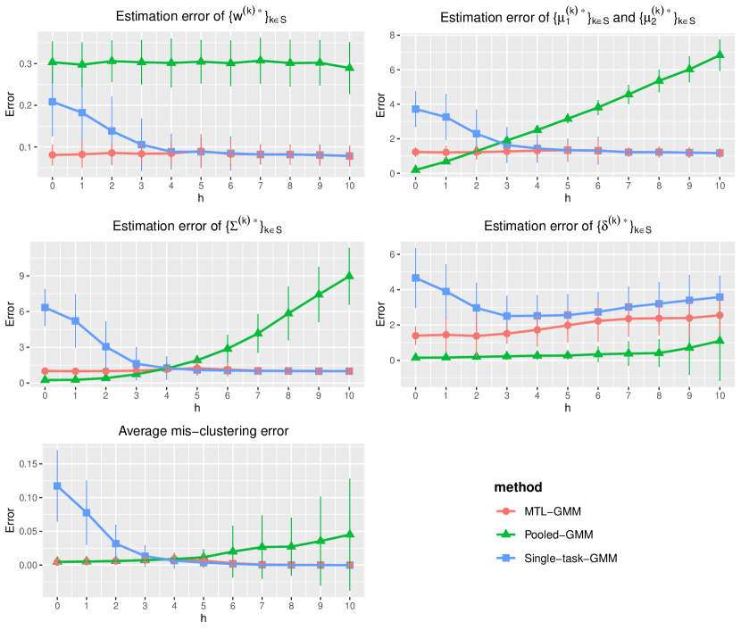
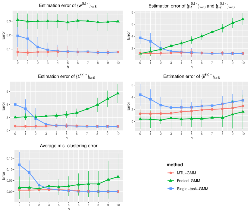
Referring to Figure S.3 for the case without outlier tasks, MTL-GMM outperforms Pooled-GMM in estimating all the time. This makes sense because Pooled-GMM does not take the heterogeneity of ’s into account. For the estimation of other parameters (except 555Actually it is not surprising to see Pooled-GMM estimates , , , and better than MTL-GMM when is small in this example. The reason is that these parameters are similar to each other (although MTL-GMM does not rely on this similarity) which makes pooling the data a good approach.) and clustering, MTL-GMM and Pooled-GMM are competitive when is small (i.e. the tasks are similar). As increases (i.e. tasks become more heterogenous), MTL-GMM starts to outperform Pooled-GMM by a large margin. Moreover, MTL-GMM is significantly better than Single-task-GMM in terms of both estimation and mis-clustering errors over a wide range of . They only become comparable when is very large. These comparisons demonstrate that MTL-GMM not only effectively utilizes the unknown similarity structure among tasks, but also adapts to it.
The results for the case with two outlier tasks are shown in Figure S.4. It is clear that the comparison between MTL-GMM and Single-task-GMM is similar to the one in Figure S.3. What is new here is that even when is very small, MTL-GMM still performs much better than Pooled-GMM, showing the robustness of MTL-GMM against a fraction of outlier tasks. Note that in this simulation, for all , which might explain the phenomenon where Pooled-GMM outperforms MTL-GMM in estimating ’s.
S.3.1.2 Simulation 2
The second simulation is a multi-cluster example, which is built based on Simulation 1. Consider a multi-task learning problem with tasks, where each task has sample size and dimension , and follows a GMM with clusters. For all , we generate independently from with . When , we generate from , where , . When , we generate each from the same Dirichlet distribution and set and from for . For a given , in each replication the outlier task index set is uniformly sampled from all subsets of with cardinality . We consider two cases:
-
(i)
No outlier tasks (), and changes from 0 to 10 with increment 1;
-
(ii)
2 outlier tasks (), and changes from 0 to 10 with increment 1.
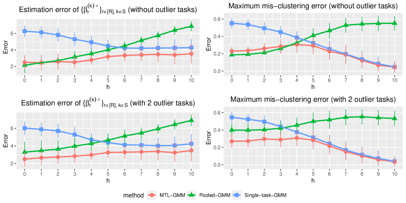
Algorithm 4 is run with the alignment Algorithm 6. The results of it and other benchmarks are reported in Figures S.5. The main message is the same as in Simulation 1: Pooled-GMM is sensitive to outlier tasks and suffers from negative transfer when is large, while MTL-GMM is robust to outliers and can adapt to the unknown similarity level . Note that in this example, are similar, and are the same, therefore running the EM algorithm by pooling all the data when is small without outliers may be more effective than our MTL algorithm. This could explain why MTL-GMM performs slightly worse than Pooled-GMM in terms of maximum mis-clustering error when is small and .
We also provide additional performance evaluations for the three methods in Simulation 2. The results are presented in Figures S.6 and S.7. The main takeaway is the same as in the previous simulation example: Pooled-GMM is sensitive to outlier tasks and suffers from negative transfer when is large, while MTL-GMM is robust to outliers and can adapt to the unknown similarity level . The results verify the theoretical findings in the multi-cluster case.
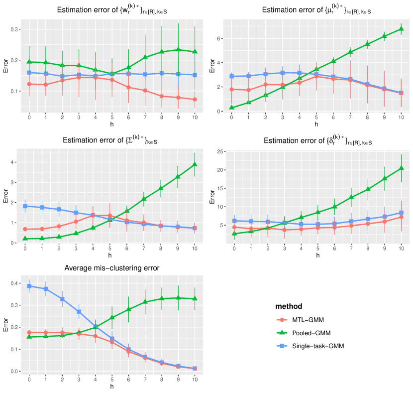
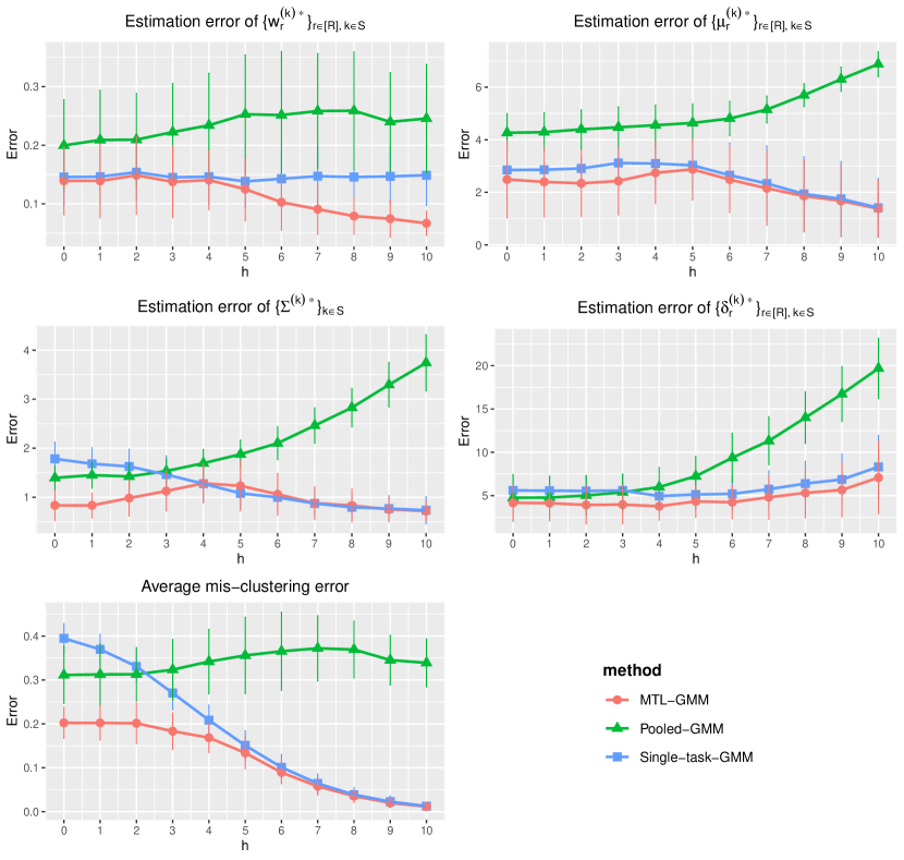
S.3.1.3 Simulation 3 of MTL
In the third simulation of MTL, we consider a different similarity structure among tasks in and a different type of outlier tasks. For a multi-task learning problem with tasks, set the sample size of each task equal to 100. Let , , and , i.e., the first task is not an outlier task. We generate each from for all . For , we generate as
| (S.3.79) |
and set . Here, the value of is determined by for a given . Let and , . In this generation process, for all . The covariance matrix of tasks in can differ. When , we generate the data of task from two clusters with probability and , where . Samples from the second cluster follow , with coming from (S.3.79), , and . For each sample from the first cluster, each component is independently generated from a -distribution with degrees of freedom . In each replication, for given , the outlier task index set is uniformly sampled from all subsets of with cardinality (since task 1 has been fixed in ). We consider two cases:
-
(i)
No outlier tasks (), and changes from 0 to 10 with increment 1;
-
(ii)
2 outlier tasks (), and changes from 0 to 10 with increment 1.
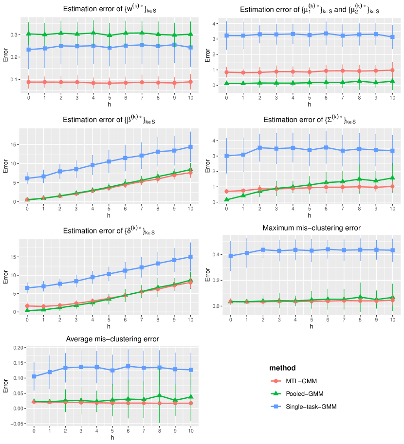
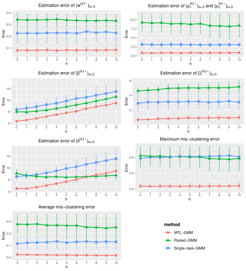
We implement the same three methods as in Simulation 1 and the results are reported in Figures S.8 and S.9. When there are no outlier tasks, both MTL-GMM and Pooled-GMM significantly outperform Single-task-GMM. Note that in this simulation, and for all , which might explain the phenomenon where Pooled-GMM outperforms MTL-GMM in estimating and ’s. When there are two outlier tasks, Figure S.9 shows that Pooled-GMM performs much worse than Single-task-GMM on most of the estimation errors of GMM parameters as well as the mis-clustering error rate. In contrast, MTL-GMM greatly improves the performance of Single-task-GMM, showing the advantage of MTL-GMM when dealing with outlier tasks and heterogeneous covariance matrices.
S.3.1.4 Simulation of TL
Consider a transfer learning problem with source data sets, where all sources are from the same GMM. The setting is modified based on Simulation 1 of MTL. The source and target sample sizes are equal to 100. For each of the source and target task, and , where , , and . We consider the case that changes from 0 to 10 with increment 1.
We compare five different methods, including Target-GMM fitted on target data only, MTL-GMM fitted on all the data, MTL-GMM-center which fits MTL-GMM on source data and outputs the estimated “center” as the target estimate 666MTL-GMM-center only appears in the comparison of estimation error of ’s., Pooled-GMM which fits a merged GMM on all the data, and our TL-GMM. The performance is evaluated by the estimation errors of , , , , , and as well as the mis-clustering error rate calculated on an independent test target data of size 500. Results are presented in Figure S.10.
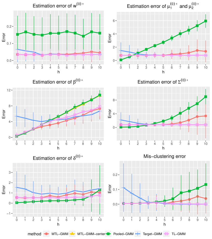
Figure S.10 shows that when is small, the performances of MTL-GMM, MTL-GMM-center, Pooled-GMM, and TL-GMM are comparable, and all of them are much better than Target-GMM. This is expected, because the sources are very similar to the target and can be easily used to improve the target task learning. As keeps increasing, the target and sources become increasingly different. This is the phase where the knowledge of sources needs to be carefully transferred for the possible learning improvement on the target task. As is clear from Figure S.10, MTL-GMM, MTL-GMM-center, and Pooled-GMM do not handle heterogeneous resources well, thus outperformed by Target-GMM. By contrast, TL-GMM remains effective in transferring source knowledge to improve over Target-GMM; when is very large so that sources are not useful anymore, TL-GMM is robust enough to still have competitive performance compared to Target-GMM.
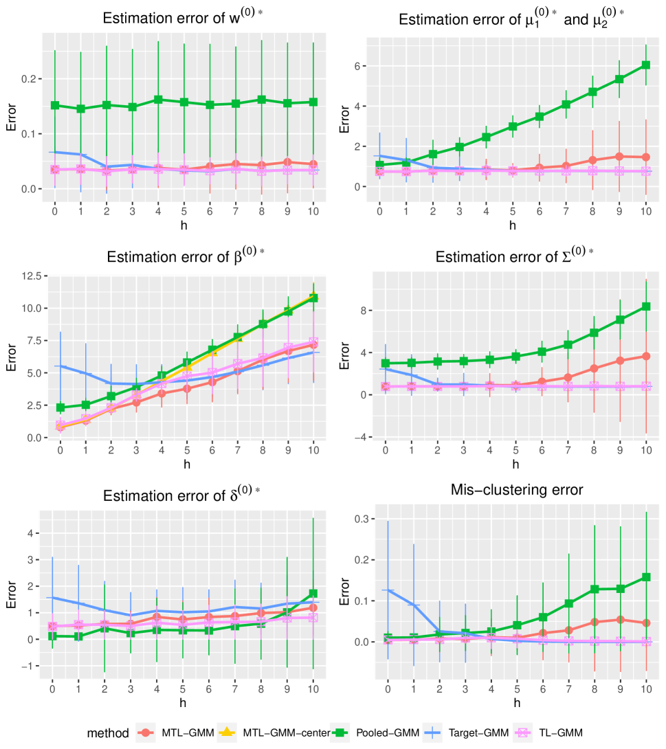
Figure S.11 shows the results when there are two outlier tasks (). It can be seen that MTL-GMM is robust to outliers.
S.3.1.5 Tuning parameters and in Algorithms 1, 4, and 7
The candidates of and values used in the 10-fold cross-validation are chosen through a data-driven way. For in Algorithm 1, we first determine the smallest value which makes all estimators identical, which is denoted as . Then the candidates are set to be the sequence from and with equal logarithm distance. For in Algorithm 7, we first determine the smallest value which makes the estimator equal to , which is denoted as . Then the candidates are set to be the sequence from and with equal logarithm distance.
We also run MTL-GMM with different values in Simulation 1 to test the impact of the penalty parameter. The results are presented in Figure S.12. The values 1.29, 2.15, 3.59, 5.99, and 10 are the last 5 elements in sequence from 0.1 to 10 with equal logarithm distance. It can be seen that with small values like 1.29 and 2.15, the performance of MTL-GMM is similar to that of Single-task-GMM, although MTL-GMM-2.15 improves Single-task-GMM a lot when is small. With large values like 5.99 and 10, MTL-GMM performs similarly to Pooled-GMM when is small while suffering from negative transfer when is large. However, as continues to increase, the performance of MTL-GMM with large values starts to improve and finally becomes similar to Single-task-GMM. This phenomenon is in accordance with the theory, as the theory predicts that MTL-GMM achieves the same rate as Single-task-GMM for large . The negative transfer effect of MTL-GMM with large could be caused by large unknown constants in the upper bound. Comparing Figure S.12 with figures in Sections 3 and S.3.1.1, we can see that cross-validation enhances the performance of MTL-GMM.
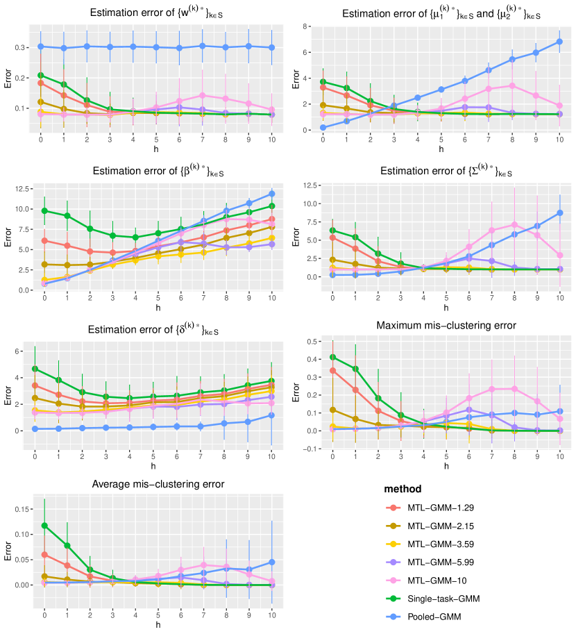
S.3.1.6 Tuning parameter and in Algorithms 1, 4, and 7
We set in Algorithms 1, 4, and 7. We run MTL-GMM with different values in Simulation 1 to test the impact of on the performance. The results are presented in Figure S.13. We tried in Algorithms 1. It can be seen that the lines representing MTL-GMM with different values highly overlap with each other, which shows that the performance of MTL-GMM is very robust to the choice of . In practice, we take for convenience.
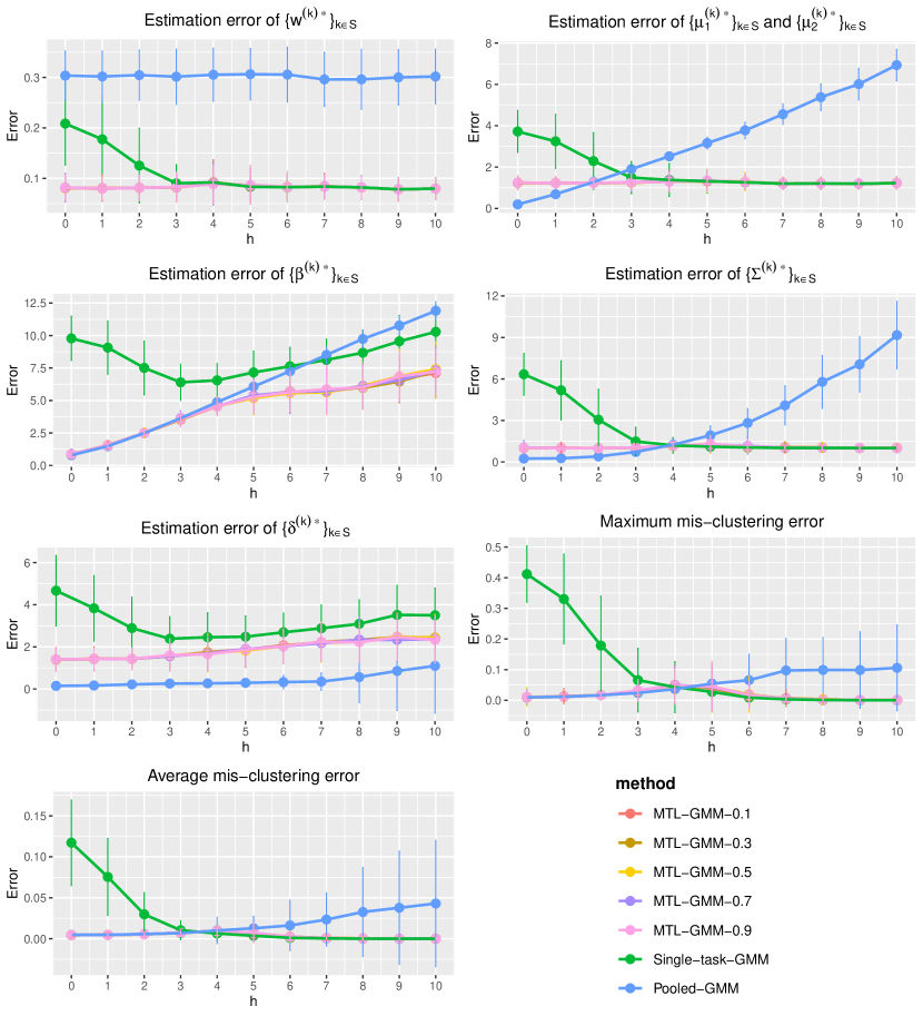
S.3.2 Real-data analysis
S.3.2.1 Human activity recognition
Human Activity Recognition (HAR) Using Smartphones Data Set contains the data collected from 30 volunteers when they performed six activities (walking, walking upstairs, walking downstairs, sitting, standing, and laying) wearing a smartphone \citepappanguita2013public. Each observation has 561 time and frequency domain variables. Each volunteer can be viewed as a task, and the sample size of each task varies from 281 to 409. The original data set is available at UCI Machine Learning Repository: https://archive.ics.uci.edu/ml/datasets/human+activity+recognition+using+smartphones.
Here, we first focus on two activities, standing and laying, and perform clustering without the label information, to test our method in the binary case. This is a binary MTL clustering problem with 30 tasks. The sample size of each task varies from 95 to 179. For each task, in each replication, we use 90% of the samples as training data and hold 10% of the samples as test data.
We first run a principal component analysis (PCA) on the training data of each task and project both the training and test data onto the first 15 principal components. PCA has often been used for dimension reduction in pre-processing the HAR data set \citepappzeng2014convolutional, walse2016pca, aljarrah2019human, duan2023adaptive. We fit Single-task-GMM on each task separately, Pooled-GMM on merged data from 30 tasks, and our MTL-GMM with the greedy label swapping alignment algorithm. The performance of the three methods is evaluated by the mis-clustering error rate on the test data of all 30 tasks. The maximum and average mis-clustering errors among the 30 tasks are calculated in each replication. The mean and standard deviation of these two errors over 200 replications are reported on the left side of Table S.1. To better display the clustering performance on each task, we further generate the box plot of mis-clustering errors of 30 tasks (averaged over 200 replications) for each method in the left plot of Figure S.14. It is clear that MTL-GMM outperforms both Pooled-GMM and Single-task-GMM.
| Binary | Multi-cluster | |||||
| Method | Single-task | Pooled | MTL | Single-task | Pooled | MTL |
| Max. error | 0.49 (0.02) | 0.40 (0.12) | 0.37 (0.09) | 0.51 (0.04) | 0.50 (0.04) | 0.51 (0.04) |
| Avg. error | 0.28 (0.02) | 0.18 (0.18) | 0.04 (0.04) | 0.25 (0.01) | 0.35 (0.03) | 0.25 (0.01) |
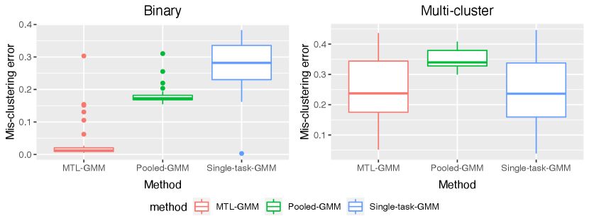
Next, we consider all six activities and compare the performance of the three approaches using the same sample-splitting strategy, to test our method in a multi-cluster scenario. Now the sample size of each task varies from 281 to 409. The maximum and average mis-clustering error rates and standard deviations over 200 replications are reported on the right side of Table S.1. We can see that Pooled-GMM might suffer from negative transfer with a worse performance than the other two methods, while MTL-GMM and Single-task-GMM have similar performances. The right plot in Figure S.14 reveals the same comparison results.
In summary, the HAR data set exhibits different levels of similarity in binary and multi-cluster cases: tasks in the binary data are sufficiently similar so that Pooled-GMM achieves a large margin of improvement over Single-task GMM, while tasks in the multi-cluster data become much more heterogeneous, resulting in the degraded performance of Pooled-GMM compared to Single-task GMM. Nevertheless, our method MTL-GMM performs either competitively or better than the best of the two, regardless of the similarity level. These results lend further support to the effectiveness of our method.
S.3.2.2 Pen-based recognition of handwritten digits (PRHD)
The Pen-based Recognition of Handwritten Digits (PRHD) data set contains 250 samples from each of the 44 writers. Each of these writers was asked to write digits 0-9 on a pressure-sensitive tablet with an integrated LCD display and a cordless stylus. The and tablet coordinates and pressure level values of the pen were recorded. After some transformations, each observation has 16 features. The data set and more information about it are available at UCI Machine Learning Repository: https://archive.ics.uci.edu/dataset/81/pen+based+recognition+of+handwritten+digits.
Similar to the previous real-data example, we first focus on a binary clustering problem by clustering observations of digits 8 and 9. The number of observations varies between 47 and 48 among the 44 tasks, showing that this is a more balanced data set with a smaller sample size (per dimension) than the HAR data. For each task, in each replication, we use 90% of the samples as training data and hold 10% of the samples as test data. The maximum and average mis-clustering error rates and standard deviations over 200 replications are reported on the left side of Table S.2, and the box plots of mis-clustering errors of 44 tasks are shown in Figure S.15. We can see that Pooled-GMM and MTL-GMM perform similarly and are much better than Single-task-GMM.
| Binary | Multi-cluster | |||||
| Method | Single-task | Pooled | MTL | Single-task | Pooled | MTL |
| Max. error | 0.32 (0.10) | 0.03 (0.07) | 0.03 (0.09) | 0.26 (0.07) | 0.37 (0.06) | 0.27 (0.07) |
| Avg. error | 0.02 (0.01) | 0.00 (0.00) | 0.00 (0.02) | 0.03 (0.01) | 0.12 (0.01) | 0.03 (0.01) |
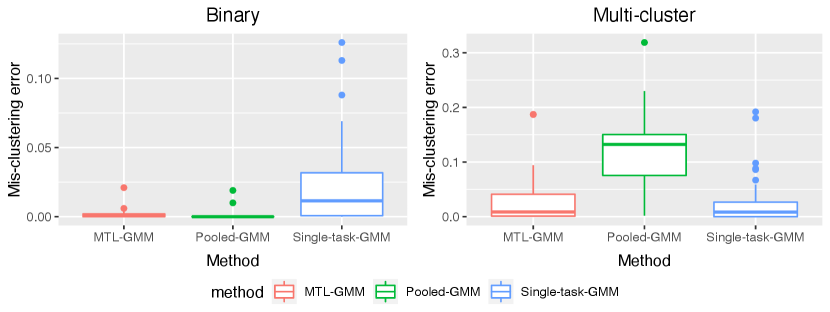
Next, we consider the observations of digits 5-9, i.e. a 5-class clustering problem. The maximum and average mis-clustering error rates and standard deviations over 200 replications are reported on the right side of Table S.2, and the box plots of mis-clustering errors of 44 tasks are shown in Figure S.15. In this multi-cluster case, MTL-GMM and Single-task-GMM have similar performance which is better than that of Pooled-GMM. Like in the first real-data example, our method MTL-GMM adapts to the unknown similarity and is competitive with the best of the other two methods.
S.4 Technical Lemmas
S.4.1 General lemmas
Denote the unit ball and the unit sphere .
Lemma 1 (Covering number of the unit ball under Euclidean norm, Example 5.8 in \citealpappwainwright2019high).
Denote the -covering number of a unit ball in under Euclidean norm as , where the centers of covering balls are required to be on the sphere. We have .
Lemma 2 (Packing number of the unit sphere under Euclidean norm).
Denote the -packing number of the unit sphere in under Euclidean norm as . When , we have .
Lemma 3 (Fano’s lemma, see Chapter 2 of \citealpapptsybakov2009introduction, Chapter 15 of \citealpappwainwright2019high).
Suppose is a metric space and each in this space is associated with a probability measure . If is an -separated set (i.e. for any ), and , then
| (S.4.80) |
where .
Lemma 4 (Packing number of the unit sphere in a quadrant under Euclidean norm).
In , we can use a vector to indicate each quadrant . Then when , there exists a quadrant such that .
Lemma 5.
For one-dimensional Gaussian mixture variable with , it is a -subGaussian variable. That means,
| (S.4.81) |
Lemma 6 (\citealpappduan2023adaptive).
Let
| (S.4.82) |
Suppose there exists such that the following conditions are satisfied:
-
(i)
For any , is -regular, that is
-
•
is convex and twice differentiable;
-
•
for all ;
-
•
.
-
•
-
(ii)
, , with .
Then we have the following conclusions:
-
(i)
for all .
-
(ii)
If
(S.4.83) where , , and , then
(S.4.84) Furthermore, if we also have
(S.4.85) then for all , and
(S.4.86)
Lemma 7.
Suppose
| (S.4.87) |
with some . Assume is convex and twice differentiable, and for any . Then
-
(i)
, for any and ;
-
(ii)
, if and .
S.5 Proofs
S.5.1 Proofs of general lemmas
S.5.1.1 Proof of Lemma 2
The second half inequality is due to Lemma 1. It suffices to show the first half inequality. For any , define . Then we can define a mapping
| (S.5.88) |
with for and . And it’s easy to see that for any , , we have . Therefore, if is an -cover of under Euclidean norm, then it must be an -cover of under Euclidean norm. Then
| (S.5.89) |
S.5.1.2 Proof of Lemma 4
If is an -packing of under Euclidean norm, then must be an -packing of under Euclidean norm. Then by Lemma 2,
| (S.5.90) | ||||
| (S.5.91) | ||||
| (S.5.92) |
implying
| (S.5.93) |
S.5.1.3 Proof of Lemma 5
Suppose , then we can write , where that is independent with and . Then
| (S.5.94) | ||||
| (S.5.95) | ||||
| (S.5.96) |
where the last second inequality comes from Jensen’s inequality and the independence between , , and . This completes the proof.
S.5.1.4 Proof of Lemma 6
The result follows from Theorem A.2, Lemma B.1, and Claim B.1 in \citeappduan2023adaptive.
S.5.2 Proof of Theorem 1
Define the contraction basin of one GMM as
| (S.5.97) | ||||
| (S.5.98) |
for which we may shorthand as in the following. And given the index set , two joint contraction basins are defined as
| (S.5.99) | ||||
| (S.5.100) |
For simplicity, at some places, we will write them as and , respectively.
For and , define
| (S.5.101) |
And denote the minimum SNR .
S.5.2.1 Lemmas
For GMM and any , define
| (S.5.102) | ||||
| (S.5.103) |
Lemma 8 (Contraction of binary GMMs, a special case of Lemma 37 when ).
When with a small constant and with a large constant , there exist positive constants and , for any ,
| (S.5.104) |
where with a constant .
Lemma 9.
When , .
Lemma 10 (Theorem 3 in \citealpappmaurer2021concentration).
Let and be a vector of independent random variables with values in a space . Then for any we have
| (S.5.105) |
where as a random function of is defined to be , the sub-Gaussian norm , and .
Lemma 11.
Suppose Assumption 1 holds.
-
(i)
With probability at least ,
(S.5.106) for all .
-
(ii)
With probability at least ,
(S.5.107)
Lemma 12.
Suppose Assumption 1 holds.
-
(i)
With probability at least ,
(S.5.108) (S.5.109) for all .
-
(ii)
With probability at least ,
(S.5.110) (S.5.111)
Lemma 13.
Suppose Assumption 1 holds.
-
(i)
With probability at least ,
(S.5.112) for all .
-
(ii)
With probability at least ,
(S.5.113) -
(iii)
With probability at least ,
(S.5.114)
Lemma 14.
Suppose Assumption 1 holds.
-
(i)
With probability at least ,
(S.5.115) for all .
-
(ii)
With probability at least ,
(S.5.116)
S.5.2.2 Main proof of Theorem 1
The proof of Theorem 1 consists of two cases. In Case 1, we study the scenario , where we take a fixed contraction radius. In this case, proving a single-task estimation error rate is sufficient, which is relatively straightforward. In Case 2, we explore the scenario , in which regime multi-task learning can outperform the classical single-task learning. In this case, the classical finite-sample analysis of EM in \citeappbalakrishnan2017statistical and \citeappcai2019chime, which uses a fixed contraction radius as we did in Case 1, does not work. This is because the heterogenous and lead to an error of when estimating . This term ultimately affects the estimation error of and , preventing us from proving the improvement of multi-task learning over single-task learning. To resolve this issue, we creatively use a “localization” strategy to adaptively shrink the contraction radius in each iteration. This method effectively eliminates the term . By combining the two cases, we complete the proof.
(\@slowromancapi@) Case 1: Let us consider the case that . Consider an event defined to be the intersection of the events in Lemmas 11.(i), 12.(i), 13.(i), and 14.(i), with a large constant , which satisfies . Throughout the analysis in Case 1, we condition on , therefore all the arguments hold with probability at least .
Consider the case . Lemma 6 tells us that when , we have
| (S.5.117) |
And if further , we have (S.5.117) holds with for all . Note that
| (S.5.118) |
And the first term on the RHS can be controlled as
| (S.5.119) | |||
| (S.5.120) | |||
| (S.5.121) | |||
| (S.5.122) |
Conditioned on , we have
| (S.5.123) |
And
| (S.5.124) | ||||
| (S.5.125) |
where
| (S.5.126) |
Before we discuss how to control the terms on the RHS, let us first try to control as it will be used to bound the existing terms. Note that by Lemma 8,
| (S.5.127) | ||||
| (S.5.128) | ||||
| (S.5.129) | ||||
| (S.5.130) |
where is a small constant. By Lemma 8 again,
| (S.5.131) | ||||
| (S.5.132) | ||||
| (S.5.133) | ||||
| (S.5.134) | ||||
| (S.5.135) | ||||
| (S.5.136) | ||||
| (S.5.137) |
Therefore, we can bound the RHS of (S.5.126) as
| (S.5.138) |
Similarly, we have
| (S.5.139) |
Combining (S.5.138) and (S.5.139), we have
| (S.5.140) |
Similarly, we can bound in the same way, and get
| (S.5.141) |
Hence
| (S.5.142) |
And the second term on the RHS of (S.5.118) satisfies
| (S.5.143) |
All together, we have
| (S.5.144) |
This implies that , therefore by (S.5.117),
| (S.5.145) |
And by (S.5.129),
| (S.5.146) |
Also,
| (S.5.147) | ||||
| (S.5.148) | ||||
| (S.5.149) |
which entails that
| (S.5.150) |
Combining (S.5.145), (S.5.146), and (S.5.150), we have
| (S.5.151) |
Also,
| (S.5.152) |
When we assume (S.5.145), (S.5.151), (S.5.152) hold for all , via the same analysis we will have (S.5.144) hold again for . Hence
| (S.5.153) |
Then by (S.5.152) when ,
| (S.5.154) | ||||
| (S.5.155) | ||||
| (S.5.156) |
where we need with a large constant . Recall that is one of the tuning parameters in the update formula of . Therefore we can follow the same arguments as above to obtain (S.5.129), (S.5.143), (S.5.145), (S.5.149), (S.5.151), (S.5.152) for .
So far, we have shown that (S.5.129), (S.5.143), (S.5.145), (S.5.149), (S.5.151), (S.5.152) hold for any . By the update formula of , when , we have
| (S.5.157) |
Therefore by (S.5.151),
| (S.5.158) | ||||
| (S.5.159) | ||||
| (S.5.160) | ||||
| (S.5.161) |
Consider a new event defined to be the intersection of the events in Lemmas 11.(i), 12.(i), 13.(i), and 14.(i), with , which satisfies . Throughout the following analysis in Case 1, we condition on , therefore all the arguments hold with probability at least . When , since , we have . Furthermore, when with a large , we have and , where we used the fact again to get the second inequality.
Then by (S.5.129),
| (S.5.165) | ||||
| (S.5.166) | ||||
| (S.5.167) | ||||
| (S.5.168) |
Similarly, by (S.5.149),
| (S.5.169) | ||||
| (S.5.170) |
Therefore,
| (S.5.171) | ||||
| (S.5.172) | ||||
| (S.5.173) | ||||
| (S.5.174) |
Combine it with (S.5.164), we obtain that
| (S.5.175) |
Plugging this back into (S.5.139), we get
| (S.5.176) |
And the same bound holds for as well. The same bound for can be obtained in the same spirit as in (S.5.122).
(\@slowromancapii@) Case 2: We now focus on the case that . As mentioned at the beginning of this proof, we need to adaptively shrink the radius of the contraction basin to prove the desired convergence rate. The analysis of Case 2 can be divided into two stages. In the first stage, we use the same fixed contraction radius as in Case 1 and follow the same analysis until the iterative error has reduced to the single-task error . In the second stage, we apply the localization argument to shrink the contraction basin until we achieve the desired rate of convergence.
Similar to Case 1, we consider an event defined to be the intersection of the events in Lemmas 11, 12, 13, and 14, with a large constant , which satisfies . Throughout the analysis in Case 2, we condition on , therefore all the arguments hold with probability at least .
Consider as the number of iterations in the first stage which satisfies . When , we can go through the same analysis as in Case 1, and show that conditioned on ,
| (S.5.177) |
and
| (S.5.178) | |||
| (S.5.179) | |||
| (S.5.180) |
Since , the rates above are the desired rates. In the following, we will derive the results for the case .
Define
| (S.5.181) | ||||
| (S.5.182) | ||||
| (S.5.183) |
Consider an event defined to be the intersection of the events in Lemmas 11, 12, 13, and 14, with , which satisfies . In the following, we condition on , therefore all the arguments hold with probability at least .
Let . Since , by Lemma 6, we also have for all . Similar to (S.5.129),
| (S.5.184) | ||||
| (S.5.185) | ||||
| (S.5.186) | ||||
| (S.5.187) |
This implies that
| (S.5.188) |
And by Lemma 6,
| (S.5.189) | ||||
| (S.5.190) |
where
| (S.5.191) | ||||
| (S.5.192) |
And the first term on the RHS can be controlled as
| (S.5.193) | |||
| (S.5.194) | |||
| (S.5.195) | |||
| (S.5.196) |
Conditioned on , we have
| (S.5.197) |
And
| (S.5.198) | ||||
| (S.5.199) |
where
| (S.5.200) |
For the first term, we have
| (S.5.201) | |||
| (S.5.202) | |||
| (S.5.203) | |||
| (S.5.204) | |||
| (S.5.205) |
where is some constant such that under event . Note that the last inequality holds because the expectation is w.r.t. which is independent of . By Lemma 13.(iii) and the definition of , the second term can be bounded as
| (S.5.206) |
Therefore,
| (S.5.207) |
On the other hand, by simple calculations, we have
| (S.5.208) | |||
| (S.5.209) | |||
| (S.5.210) | |||
| (S.5.211) | |||
| (S.5.212) | |||
| (S.5.213) | |||
| (S.5.214) | |||
| (S.5.215) |
Hence
| (S.5.216) |
A similar discussion leads to the same bound for . Therefore,
| (S.5.217) |
And the same bound holds for , which can be shown in the same spirit. Putting all the pieces together,
| (S.5.218) |
Therefore by Lemma 6 and (S.5.190), we have for all , and
| (S.5.219) | ||||
| (S.5.220) | ||||
| (S.5.221) | ||||
| (S.5.222) |
This entails that
| (S.5.223) |
This implies that
| (S.5.224) |
Also,
| (S.5.225) | ||||
| (S.5.226) | ||||
| (S.5.227) | ||||
| (S.5.228) | ||||
| (S.5.229) | ||||
| (S.5.230) | ||||
| (S.5.231) | ||||
| (S.5.232) |
Therefore,
| (S.5.233) | ||||
| (S.5.234) |
Hence
| (S.5.235) | ||||
| (S.5.236) | ||||
| (S.5.237) | ||||
| (S.5.238) |
and
| (S.5.239) | ||||
| (S.5.240) | ||||
| (S.5.241) | ||||
| (S.5.242) | ||||
| (S.5.243) | ||||
| (S.5.244) |
where .
Therefore, for , where hence , we have updating formulas (S.5.222) and (S.5.223) for . We can get
| (S.5.245) | ||||
| (S.5.246) | ||||
| (S.5.247) |
and
| (S.5.248) | ||||
| (S.5.249) | ||||
| (S.5.250) |
with
| (S.5.251) |
where the last inequality is due to .
Consider an event series each of which is defined to be the intersection of the events in Lemmas 11, 12, 13, and 14, with , which satisfies hence . In the following, we condition on , therefore all the arguments hold with probability at least . Therefore, for , we have (S.5.244) hold, which leads to
| (S.5.252) | ||||
| (S.5.253) | ||||
| (S.5.254) | ||||
| (S.5.255) | ||||
| (S.5.256) | ||||
| (S.5.257) | ||||
| (S.5.258) |
where , which provides the desired rate for . When , by (S.5.251), we have
| (S.5.259) | ||||
| (S.5.260) |
which is the desired rate. We complete the proof for Theorem 1.
S.5.2.3 Proofs of lemmas
Proof of Lemma 11.
We prove part (i) first.
Denote . By bounded difference inequality,
| (S.5.261) |
with probability at least . By the generalized symmetrization inequality (Proposition 4.11 in \citeappwainwright2019high), with i.i.d. Rademacher variables ,
| (S.5.262) | ||||
| (S.5.263) | ||||
| (S.5.264) |
where . Denote . By the contraction inequality for Rademecher variables (Theorem 11.6 in \citealpappboucheron2013concentration),
| RHS of (S.5.261) | (S.5.266) | |||
| (S.5.267) | ||||
| (S.5.268) | ||||
| (S.5.269) | ||||
| (S.5.270) | ||||
| (S.5.271) | ||||
| (S.5.272) |
Since and are i.i.d. sub-Gaussian variables, we know that
| (S.5.273) |
Suppose is a -cover of with (see Example 5.8 in \citealpappwainwright2019high). Hence by standard arguments,
| (S.5.274) | |||
| (S.5.275) |
Again, since are i.i.d. sub-Gaussian variables,
| (S.5.276) |
Putting all the pieces together,
| (S.5.277) |
Combining (S.5.261) and (S.5.277), we get the result in (i).
Next, we derive part (ii) using a similar analysis.
Denote .
By a similar standard symmetrization and contraction arguments we used in part (i), with i.i.d. Rademacher variables , for any , we have
| (S.5.278) | |||
| (S.5.279) | |||
| (S.5.280) | |||
| (S.5.281) | |||
| (S.5.282) | |||
| (S.5.283) |
where . Denote . Suppose is a -cover of with . Then by Cauchy-Schwarz inequality and standard arguments,
| (S.5.284) | |||
| (S.5.285) | |||
| (S.5.286) | |||
| (S.5.287) | |||
| (S.5.288) | |||
| (S.5.289) | |||
| (S.5.290) | |||
| (S.5.291) | |||
| (S.5.292) | |||
| (S.5.293) |
Since , , and are independent sub-Gaussian variables, we can bound the three terms on the RHS as
| (S.5.294) | ||||
| (S.5.295) | ||||
| (S.5.296) |
Putting all pieces together,
| (S.5.297) |
Therefore, for any
| (S.5.298) |
Let and , we have
| (S.5.299) |
which completes the proof. ∎
Proof of Lemma 12.
The proof of part (ii) is the same as the proof of part (ii) for Lemma 11, so we omit it. The only difference between the proofs of part (i) for two lemmas is that here the bounded difference inequality is not available. Denote
| (S.5.300) |
We need to use Lemma 10 to upper bound . Prior to that, we first verify the conditions required by the lemma. Fix , …, , , …, , and define
| (S.5.301) |
By triangle inequality,
| (S.5.302) | |||
| (S.5.303) | |||
| (S.5.304) | |||
| (S.5.305) |
Note that , where
| (S.5.306) | ||||
| (S.5.307) | ||||
| (S.5.308) |
Therefore . Hence by applying Lemma 10, we have
| (S.5.309) |
with probability at least . ∎
Proof of Lemma 13.
For part (i), denote
| (S.5.310) |
Suppose is a -cover of with . Define . Then by the generalized symmetrization inequality (Proposition 4.11 in \citealpappwainwright2019high), with i.i.d. Rademacher variables , for any ,
| (S.5.311) | |||
| (S.5.312) | |||
| (S.5.313) | |||
| (S.5.314) | |||
| (S.5.315) | |||
| (S.5.316) | |||
| (S.5.317) | |||
| (S.5.318) | |||
| (S.5.319) | |||
| (S.5.320) |
Note that since are i.i.d. sub-exponential variables and are i.i.d. sub-Gaussian variables, we have
| (S.5.321) | ||||
| (S.5.322) |
where the first inequality holds when where is small. Therefore,
| (S.5.323) |
when . The desired result follows from Chernoff’s bound.
The proofs of parts (ii) and (iii) are almost the same as the proofs of part (ii) of Lemma 11, so we do not repeat them here.
∎
Proof of Lemma 14.
Note that
| (S.5.324) |
The bound of the RHS comes from Theorem 6.5 in \citeappwainwright2019high. And the bound in part (ii) can be proved in the same way. ∎
S.5.3 Proof of Theorem 3
S.5.3.1 Lemmas
Recall the parameter space
| (S.5.325) |
where and .
Lemma 15 (Lemma 8.4 in \citealpappcai2019chime).
For any , and , denote and . Then
| (S.5.326) |
Lemma 16.
For any , , , and , denote and . Then
| (S.5.327) |
Lemma 17.
Denote distribution as for any , where . Then
| (S.5.328) |
Lemma 18.
Denote distribution as for any . Then
| (S.5.329) |
Lemma 19.
When there exists an subset such that with some constant , we have
| (S.5.330) | ||||
| (S.5.331) |
Lemma 20.
Denote . Then
| (S.5.332) |
Lemma 21 (The first variant of Theorem 5.1 in \citealpappchen2018robust).
Given a series of distributions , each of which is indexed by the same parameter . Consider independently for . Denote the joint distribution of as . Then
| (S.5.333) |
where .
Lemma 22.
Suppose . Consider two data generating mechanisms:
-
(i)
independently for , where ;
-
(ii)
With a preserved set , generate and independently for .
Denote the joint distributions of in (i) and (ii) as and , respectively. We claim that if
| (S.5.334) |
then
| (S.5.335) |
where for any .
Lemma 23.
When there exists an subset such that with some constant , we have
| (S.5.336) | |||
| (S.5.337) |
S.5.3.2 Main proof of Theorem 3
S.5.3.3 Proofs of lemmas
Proof of Lemma 17.
Denote , , and .
By Taylor expansion,
| (S.5.338) |
where is between and . By the property of score function,
| (S.5.339) |
Besides,
| (S.5.340) |
where . Note that
| (S.5.341) |
for any . Therefore,
| (S.5.342) | ||||
| (S.5.343) | ||||
| (S.5.344) |
which completes the proof. ∎
Proof of Lemma 18.
Recall that we denote distribution as for any . By the bi-convexity of KL divergence, we have
| (S.5.345) | ||||
| (S.5.346) | ||||
| (S.5.347) |
which completes the proof. ∎
Proof of Lemma 19.
WLOG, suppose . It’s easy to see that given any , , where
| (S.5.348) | ||||
| (S.5.349) | ||||
| (S.5.350) | ||||
| (S.5.351) |
(i) By fixing an and a , we want to show
| (S.5.352) |
By Lemma 4, a quadrant of and a -packing of under Euclidean norm: , where with a small constant and when . For any , denote distribution as , where can be any vector in with . Then
| LHS | (S.5.353) | |||
| (S.5.354) |
where the last inequality holds because it suffices to consider estimator satisfying almost surely. In addition, for any , , .
(ii) By fixing an and a , we want to show
| (S.5.361) |
WLOG, suppose . We have
| (S.5.362) |
By Lemma 4, a quadrant of and a -packing of under Euclidean norm: , where with a small constant and when . WLOG, assume . Denote . Let for all . And let with . For any , denote distribution as . Then similar to the arguments in (i),
| LHS | (S.5.363) | |||
| (S.5.364) |
Then by Lemma 15,
| (S.5.365) | ||||
| (S.5.366) | ||||
| (S.5.367) | ||||
| (S.5.368) | ||||
| (S.5.369) |
when and . By Fano’s lemma (See Corollary 2.6 in \citealpapptsybakov2009introduction),
| (S.5.370) |
when , and .
(iii) By fixing an and a , we want to show
| (S.5.371) |
Suppose and denote the associated quadrant , . Let with a small constant for . For any , where , denote distribution as , and the joint distribution of and as . And denote distribution as for any . Similar to the arguments in (i), since it suffices to consider the estimators satisfying almost surely and for any , , we have
| LHS | (S.5.372) | |||
| (S.5.373) | ||||
| (S.5.374) |
Consider where for and , where . Define two new “distances” (which are not rigorously distances because triangle inequalities and the definiteness do not hold) between and as
| (S.5.375) | ||||
| (S.5.376) |
Therefore when . For , define . Because for any , and , it’s easy to see that
| (S.5.377) | |||
| (S.5.378) | |||
| (S.5.379) | |||
| (S.5.380) |
By Lemma 15,
| (S.5.381) | ||||
| (S.5.382) | ||||
| (S.5.383) | ||||
| (S.5.384) | ||||
| (S.5.385) | ||||
| (S.5.386) |
when . By Fano’s lemma (See Corollary 2.6 in \citealpapptsybakov2009introduction),
| (S.5.387) |
when , , and .
(iv) We want to show
| (S.5.388) | ||||
| (S.5.389) |
The argument is similar to part (iii). The only two differences here are that the dimension of interested parameter equals 1, and Lemma 15 is replaced by Lemma 17.
(v) We want to show
| (S.5.390) | ||||
| (S.5.391) |
The argument is similar to (iii). The only two differences here are that the dimension of interested parameter equals 1, and Lemma 15 is replaced by Lemma 18.
Finally, we get the desired conclusion by combining (i)-(v). ∎
Proof of Lemma 20.
Proof of Lemma 21.
The proof is similar to the proof of Theorem 5.1 in \citeappchen2018robust, so we omit it here. ∎
Proof of Lemma 22.
It’s easy to see that
| (S.5.394) |
where can be any probability measure on all subsets of with .
Consider a special distribution as :
| (S.5.395) |
for any with . Given , consider the distribution of as
| (S.5.396) |
Then consider the distribution of as
| (S.5.397) |
It’s easy to see that is the same as conditioning on the event . Therefore,
| (S.5.398) | |||
| (S.5.399) | |||
| (S.5.400) | |||
| (S.5.401) | |||
| (S.5.402) | |||
| (S.5.403) | |||
| (S.5.404) | |||
| (S.5.405) |
where the last third inequality comes from Bernstein’s inequality, application of Lemma 17 and the fact that . ∎
Proof of Lemma 23.
(i) We want to show
| (S.5.406) |
Fix and some . WLOG, assume . Then it suffices to show
| (S.5.407) |
Consider a special subset of as
| (S.5.408) |
where
| (S.5.409) |
and is a small constant which we will specify later. For any , denote as . Therefore it suffices to show
| (S.5.410) |
Note that for any , we can define . Then by triangle inequality and definition of , . Therefore
| (S.5.411) |
Let where is a small constant. Since for any and , by Lemma D.2 in \citeappduan2023adaptive,
| (S.5.412) |
Applying Assouad’s lemma (Theorem 2.12 in \citealpapptsybakov2009introduction or Lemma 2 in \citealpappcai2012optimal), we get
| (S.5.413) | ||||
| (S.5.414) |
where is the Hamming distance. For the first term on the RHS, it’s easy to see that
| (S.5.415) |
for any and . For the second term, by the density form of Gaussian distribution, we can show that if , then
| (S.5.416) | ||||
| (S.5.417) | ||||
| (S.5.418) | ||||
| (S.5.419) |
Plugging this back into (S.5.414), combining with (S.5.412), we have
| (S.5.420) |
when and .
(ii) We want to show
| (S.5.421) |
The proof idea is similar to part (iii) of the proof of Lemma 19, so we omit the details here. It suffices to consider where when and .
∎
S.5.4 Proof of Theorem 2
We claim that with probability at least ,
| (S.5.422) |
Then the conclusion immediately follows from Theorem 1. Hence it suffices to verify the claim. For convenience, we write simply as and as .
By simple calculations, we have
| (S.5.423) | ||||
| (S.5.424) | ||||
| (S.5.425) | ||||
| (S.5.426) |
Then by Taylor expansion,
| (S.5.427) | |||
| (S.5.428) | |||
| (S.5.429) | |||
| (S.5.430) | |||
| (S.5.431) | |||
| (S.5.432) |
Denote and . By plugging in the density formula of standard Gaussian distribution, it is easy to see that
| (S.5.433) | ||||
| (S.5.434) | ||||
| (S.5.435) | ||||
| (S.5.436) | ||||
| (S.5.437) | ||||
| (S.5.438) | ||||
| (S.5.439) | ||||
| (S.5.440) |
with probability at least , where and , so . Only the last inequality in (S.5.440) holds with high probability and the others are deterministic. It comes from the fact that for some with probability at least and a direct application of Lemma 8.1 in \citeappcai2019chime. On the other hand, it is easy to see that . Combining these two facts leads to (S.5.422).
S.5.5 Proof of Theorem 4
S.5.5.1 Lemmas
Recall that for GMM associated with parameter set , we define the mis-clustering error rate of any classifier as , where represents the distribution of , i.e. . Denote as the Bayes classifier corresponding to . Define a surrogate loss .
Lemma 24.
Assume there exists an subset such that and with some constants . We have
| (S.5.441) | ||||
| (S.5.442) |
Lemma 25.
Suppose satisfies with some constant and . Then such that
| (S.5.443) |
for any classifier , where , , and is the corresponding Bayes classifier.
Lemma 26.
Consider and satisfies with some constant .. We have
| (S.5.444) |
for some constants , .
Lemma 27.
Consider and satisfies , , , , , , , , and . We have
| (S.5.445) |
for some constants , .
Lemma 28.
Denote . We have
| (S.5.446) |
S.5.5.2 Main proof of Theorem 4
S.5.5.3 Proof of lemmas
Proof of Lemma 24.
Recall the definitions and proof idea of Lemma 19. We have , where
| (S.5.447) | ||||
| (S.5.448) | ||||
| (S.5.449) | ||||
| (S.5.450) | ||||
| (S.5.451) |
Recall the mis-clustering error for GMM associated with parameter set of any classifier is . To help the analysis, following \citeappazizyan2013minimax and \citeappcai2019chime, we define a surrogate loss , where is the Bayes classifier. Suppose .
(i) We want to show
| (S.5.452) |
Consider and space . And
| (S.5.453) |
Let with some small constant . For any , denote distribution as . Consider a -packing of : . By Lemma 2, . Denote , where . Then by definition of KL divergence and Lemma 8.4 in \citeappcai2019chime,
| (S.5.454) | ||||
| (S.5.455) | ||||
| (S.5.456) | ||||
| (S.5.457) | ||||
| (S.5.458) |
For simplicity, we write with and as . By Lemma 8.5 in \citeappcai2019chime,
| (S.5.459) |
where . The last inequality holds because and when . Then by Lemma 3.5 in \citeappcai2019chime (Proposition 2 in \citealpappazizyan2013minimax), for any classifier , and ,
| (S.5.460) |
For any , consider a test . Therefore if there exists such that , then by (S.5.460), we must have . Let , then by Fano’s lemma (Corollary 6 in \citealpapptsybakov2009introduction)
| (S.5.461) | ||||
| (S.5.462) | ||||
| (S.5.463) | ||||
| (S.5.464) | ||||
| (S.5.465) |
(ii) We want to show
| (S.5.466) |
Fixing an and a . Suppose . We have
| (S.5.467) |
Let with a small constant . For any , denote distribution as . Consider a -packing of . By Lemma 2, . Denote . WLOG, assume . Let for all . Then by following the same arguments in (i) and part (ii) of the proof of Lemma 19, we can show that the RHS of (S.5.467) is larger than or equal to when .
(iii) We want to show
| (S.5.468) |
This can be proved by following similar ideas used in step (iii) of the proof of Lemma 19, so we omit the proof here.
(iv) We want to show
| (S.5.469) |
This can be similarly proved by following the arguments in part (i) with Lemmas 25 and 26.
(v) We want to show
| (S.5.470) |
This can be similarly proved by following the arguments in part (i) with Lemmas 25 and 27.
Finally, we get the desired conclusion by combining (i)-(v). ∎
Proof of Lemma 25.
We follow a similar proof idea used in the proof of Lemma 3.4 in \citeappcai2019chime. Let and be the density of and , respectively. Denote and for any classifier . Note that . The permutation actually doesn’t matter in the proof. WLOG, we drop the permutations in the definition of misclassification error and surrogate loss by assuming to be the identity function. If is not identity in the definition of , for example, we can define instead and all the following steps still follow.
By definition,
| (S.5.471) | ||||
| (S.5.472) |
which leads to
| (S.5.473) | ||||
| (S.5.474) | ||||
| (S.5.475) | ||||
| (S.5.476) | ||||
| (S.5.477) | ||||
| (S.5.478) | ||||
| (S.5.479) |
where we let with . This completes the proof. The last second inequality depends on the fact that
| (S.5.480) |
holds for all . This is because
| (S.5.481) | |||
| (S.5.482) | |||
| (S.5.483) | |||
| (S.5.484) | |||
| (S.5.485) | |||
| (S.5.486) | |||
| (S.5.487) | |||
| (S.5.488) | |||
| (S.5.489) |
when . Note that (S.5.489) implies that a binary GMM under the separation assumption has Tsybakov’s margin with margin parameter . For the notion of Tsybakov’s margin, see \citeappaudibert2007fast. We will prove a more general result showing that a multi-cluster GMM under the separation assumption also has Tsybakov’s margin with margin parameter . This turns out to be useful in proving the upper and lower bounds of misclassification error. ∎
Proof of Lemma 26.
WLOG, suppose . Similar to (S.5.486), it’s easy to see that
| (S.5.490) | ||||
| (S.5.491) | ||||
| (S.5.492) | ||||
| (S.5.493) | ||||
| (S.5.494) |
On the other hand,
| (S.5.495) | ||||
| (S.5.496) |
which completes the proof. ∎
Proof of Lemma 28.
By Lemma 25, it suffices to prove
| (S.5.497) |
For any , denote distribution as . For simplicity, we write with satisfying , and as . Consider as a loss function between and in Lemmas 21 and 22. Considering , by Lemma 15, note that
| (S.5.498) |
By Lemma 8.5 in \citeappcai2019chime, this implies for some constants
| (S.5.499) | |||
| (S.5.500) | |||
| (S.5.501) | |||
| (S.5.502) |
S.5.6 Proof of Theorem 5
Denote . WLOG, assume and for all . Hence . For any , define
| (S.5.503) | ||||
| (S.5.504) | ||||
| (S.5.505) |
WLOG, it suffices to prove that
| (S.5.506) | |||
| (S.5.507) |
In fact, if this holds, then we must have
| (S.5.508) |
Otherwise, according to (S.5.506), if , by replacing the first entries of with , we get a different alignment whose score is smaller than the score of , which is contradicted with the definition of . If , based on (S.5.507), by replacing the first entries of with , we get a different alignment whose score is smaller than the score of , which is again contradicted with the definition of .
In the following, we prove (S.5.506). The proof of (S.5.507) is almost the same, so we do not repeat it. Under the conditions we assume, it can be shown that
| (S.5.509) | ||||
| (S.5.510) | ||||
| (S.5.511) | ||||
| (S.5.512) | ||||
| (S.5.513) | ||||
| (S.5.514) |
And
| (S.5.515) | ||||
| (S.5.516) | ||||
| (S.5.517) | ||||
| (S.5.518) |
| (S.5.519) |
Combining all these pieces,
| (S.5.520) | |||
| (S.5.521) | |||
| (S.5.522) | |||
| (S.5.523) | |||
| (S.5.524) |
where (S.5.523) holds because and (S.5.524) is due to the condition (ii).
S.5.7 Proof of Theorem 6
Denote . WLOG, assume and for all . Hence . For any , define
| (S.5.525) | ||||
| (S.5.526) |
By the definition of , we must have or . If and we have
| (S.5.527) |
then for each in the for loop of Algorithm 3, the algorithm will flip the sign of to decrease the mis-alignment proportion . Then after the for loop, the mis-alignment proportion will become zero, which means the correct alignment is achieved. The case that can be similarly discussed.
Now we derive (S.5.527). Similar to the decomposition in (S.5.514), we have
| (S.5.528) | ||||
| (S.5.529) | ||||
| (S.5.530) | ||||
| (S.5.531) |
Note that
| (S.5.532) | ||||
| (S.5.533) | ||||
| (S.5.534) | ||||
| (S.5.535) |
| (S.5.536) |
| (S.5.537) |
Putting all pieces together,
| (S.5.538) | |||
| (S.5.539) | |||
| (S.5.540) | |||
| (S.5.541) |
where (S.5.540) holds because and (S.5.541) is due to the condition (iii).
S.5.8 Proof of Theorem 13
S.5.8.1 Lemmas
Define the contraction basin of one GMM as
| (S.5.542) |
for which we may shorthand as in the following.
For GMM and any , define
| (S.5.543) | ||||
| (S.5.544) |
Lemma 29.
Suppose Assumption 3 holds.
-
(i)
With probability at least ,
(S.5.545) -
(ii)
With probability at least ,
(S.5.546) -
(iii)
With probability at least ,
(S.5.547)
S.5.8.2 Main proof of Theorem 13
(\@slowromancapi@) Case 1: We first consider the case that . Consider an event defined to be the intersection of the events in Lemma 29, with a large constant , which satisfies . Throughout the analysis in Case 1, we condition on , therefore all the arguments hold with probability at least .
Similar to our analysis in the proof of Theorem 1, conditioned on , we have
| (S.5.548) | ||||
| (S.5.549) | ||||
| (S.5.550) |
Hence
| (S.5.551) | ||||
| (S.5.552) |
By Lemma 7, we have
| (S.5.553) | ||||
| (S.5.554) |
Combining these results, we have
| (S.5.555) |
By the construction of , we know that
| (S.5.556) |
implies that
| (S.5.557) | ||||
| (S.5.558) | ||||
| (S.5.559) |
which is the desired rate. The bound of and can be derived similar to (S.5.549) and (S.5.550).
(\@slowromancapii@) Case 2: Next, we consider the case that . According to Assumption 3, we have . It is easy to see that the analysis in part (\@slowromancapi@) does not depend on the condition . Hence we have proved the desired bounds of and . Denote as an integer such that . When , the bound in part (\@slowromancapi@) is the desired bound since the term dominates the other terms. Let us consider the case .
Consider an event defined to be the event of
| (S.5.560) |
Note that since , by part (\@slowromancapii@) of the proof of Theorem 1, we know that . And implies that
| (S.5.561) |
where the second inequality comes from Assumption 3.
Also consider another event defined to be the intersection of the events in Lemma 29, with , which satisfies . Throughout the analysis in Case 1, we condition on , therefore all the arguments hold with probability at least .
Note that and . Hence by Lemma 7, we have thus
| (S.5.562) |
Similar to the analysis in part (\@slowromancapii@) in the proof of Theorem 1, we have
| (S.5.563) | ||||
| (S.5.564) | ||||
| (S.5.565) | ||||
| (S.5.566) |
Putting all pieces together,
| (S.5.567) |
We can continue this analysis from to , and so on. Hence for any , we have
| (S.5.568) | ||||
| (S.5.569) | ||||
| (S.5.570) | ||||
| (S.5.571) | ||||
| (S.5.572) | ||||
| (S.5.573) |
where the last inequality holds because is chosen to be the integer satisfying .
S.5.8.3 Proof of lemmas
S.5.9 Proof of Theorem 15
S.5.9.1 Lemmas
Recall
| (S.5.574) |
Lemma 30.
When with some constant , we have
| (S.5.575) |
Lemma 31.
Denote . Then
| (S.5.576) |
Lemma 32 (The second variant of Theorem 5.1 in \citealpappchen2018robust).
Given a series of distributions , each of which is indexed by the same parameter . Consider independently for and . Denote the joint distribution of as . Then
| (S.5.577) |
where .
Lemma 33.
Consider two data generating mechanisms:
-
(i)
independently for and , where ;
-
(ii)
With a preserved set , generate and independently for . And .
Denote the joint distributions of in (i) and (ii) as and , respectively. We claim that if
| (S.5.578) |
then
| (S.5.579) |
where for any .
Lemma 34.
When with some constant , we have
| (S.5.580) |
S.5.9.2 Main proof of Theorem 15
S.5.9.3 Proof of lemmas
Proof of Lemma 30.
It’s easy to see that , where
| (S.5.581) | ||||
| (S.5.582) | ||||
| (S.5.583) | ||||
| (S.5.584) |
(i) By fixing an and a , we want to show
| (S.5.585) |
By Lemma 4, a quadrant of and a -packing of under Euclidean norm: , where with a small constant and when . For any , denote distribution as . Then
| LHS | (S.5.586) | |||
| (S.5.587) |
where the last inequality holds because it suffices to consider estimator satisfying almost surely. In addition, for any , , .
(ii) By fixing an and a , we want to show
| (S.5.594) |
By Lemma 4, a quadrant of and a -packing of under Euclidean norm: , where with a small constant and when . WLOG, assume . Denote . Let for all and with . For any , denote distribution as . Then similar to the arguments in (i),
| LHS | (S.5.596) | |||
| (S.5.597) |
Then by Lemma 15,
| (S.5.598) | ||||
| (S.5.599) | ||||
| (S.5.600) | ||||
| (S.5.601) | ||||
| (S.5.602) |
when and . By Fano’s lemma (See Corollary 2.6 in \citealpapptsybakov2009introduction),
| (S.5.603) |
when , and .
(iii) We want to show
| (S.5.604) |
The argument is similar to (ii). The only two differences here are that the dimension of interested parameter equals 1, and Lemma 15 is replaced by Lemma 17.
(iv) We want to show
| (S.5.605) |
The argument is similar to (ii).
Finally, we get the desired conclusion by combining (i)-(iv).
∎
Proof of Lemma 31.
Let and . Since , . Denote . For any , denote distribution as , and denote as . It suffices to show
| (S.5.606) |
where .
Proof of Lemma 32.
The proof is similar to the proof of Theorem 5.1 in \citeappchen2018robust, so we omit it here. ∎
S.5.10 Proof of Theorem 14
S.5.11 Proof of Theorem 16
S.5.11.1 Lemmas
Lemma 35.
Assume and with some constants , . We have
| (S.5.608) |
Lemma 36.
Denote . We have
| (S.5.609) |
S.5.11.2 Main proof of Theorem 16
S.5.11.3 Proof of lemmas
Proof of Lemma 35.
We proceed with similar proof ideas used in the proof of Lemma 35. Recall the definitions and proof idea of Lemma 30. We have , where
| (S.5.610) | ||||
| (S.5.611) | ||||
| (S.5.612) | ||||
| (S.5.613) |
Recall the mis-clustering error for GMM associated with parameter set of any classifier is . To help the analysis, following \citeappazizyan2013minimax and \citeappcai2019chime, we define a surrogate loss , where is the Bayes classifier. Suppose .
(i) We want to show
| (S.5.614) |
Consider and space . And
| (S.5.615) |
Let with some small constant . For any , denote distribution as . Consider a -packing of : . By Lemma 2, . Denote , where . Then by definition of KL divergence and Lemma 8.4 in \citeappcai2019chime,
| (S.5.616) | ||||
| (S.5.617) | ||||
| (S.5.618) | ||||
| (S.5.619) | ||||
| (S.5.620) |
For simplicity, we write with and as . By Lemma 8.5 in \citeappcai2019chime,
| (S.5.621) |
where . The last inequality holds because and when . Then by Lemma 3.5 in \citealpappcai2019chime (Proposition 2 in \citeappazizyan2013minimax), for any classifier , and ,
| (S.5.622) |
For any , consider a test . Therefore if there exists such that , then by (S.5.622), we must have . Let , then by Fano’s lemma (Corollary 6 in \citealpapptsybakov2009introduction)
| (S.5.623) | ||||
| (S.5.624) | ||||
| (S.5.625) | ||||
| (S.5.626) | ||||
| (S.5.627) |
(ii) We want to show
| (S.5.628) |
Fixing an and a . Suppose . We have
| (S.5.629) |
Let with a small constant . For any , denote distribution as . Consider a -packing of . By Lemma 2, . Denote . WLOG, assume . Let for all and with . Then by following the same arguments in part (ii) of the proof of Lemma 30, we can show that the RHS of (S.5.629) is larger than or equal to when .
(iii) We want to show
| (S.5.630) |
This can be similarly proved by following the arguments in part (i) with Lemmas 25 and 26.
(iv) We want to show
| (S.5.631) |
The conclusion can be obtained immediately from (ii), by noticing that .
Finally, we get the desired conclusion by combining (i)-(iv). ∎
Proof of Lemma 36.
By Lemma 25, it suffices to prove
| (S.5.632) |
For any , denote distribution as . For simplicity, we write with satisfying , and as . Consider as a loss function between and in Lemmas 32 and 33. Considering , by Lemma 15, note that
| (S.5.633) | ||||
| (S.5.634) |
By Lemma 8.5 in \citeappcai2019chime, this implies for some constants
| (S.5.635) | |||
| (S.5.636) | |||
| (S.5.637) | |||
| (S.5.638) |
S.5.12 Proof of Theorem 17
Denote . WLOG, assume and for all . Hence . WLOG, consider for all (i.e., the tasks in are already well-aligned). Consider
| (S.5.639) | ||||
| (S.5.640) |
It suffices to prove that
| (S.5.641) |
In fact,
| (S.5.642) | ||||
| (S.5.643) |
where
| (S.5.644) | ||||
| (S.5.645) | ||||
| (S.5.646) |
and
| (S.5.647) |
Hence
| (S.5.648) | ||||
| (S.5.649) | ||||
| (S.5.650) |
when , which completes our proof.
S.5.13 Proof of Theorem 7
Define the contraction basin of one GMM as
| (S.5.651) | ||||
| (S.5.652) |
And the joint contraction basin is defined as .
For and , define
| (S.5.653) |
S.5.13.1 Lemmas
For GMM and any , define
| (S.5.654) |
Denote and .
Lemma 37 (Contraction of multi-cluster GMM).
When with a small constant and with a large constant , there exist positive constants and , for any ,
| (S.5.655) |
where with a constant .
Lemma 38 (Vectorized contraction of Rademacher complexity, Corollary 1 in \citealpappmaurer2016vector).
Suppose and are independent Rademacher variables. Let be a class of functions and is -Lipschitz under -norm, i.e., , where , . Then
| (S.5.656) |
where is the -th component of .
S.5.13.2 Main proof of Theorem 7
The proof idea is almost the same as the idea used in the proof of Theorem 1. We still need to show similar results presented in the lemmas associated with Theorem 1, then go through the same arguments in the proof of Theorem 7. We only sketch the key steps and the differences here.
The biggest difference appears in the proofs of the lemmas associated with Theorem 1 under the context of multi-cluster GMM. The original arguments in the proofs of Lemmas 11-14 involve the contraction inequality for Rademacher variables and univariate Lipschitz functions, which is not available anymore. We replace this part with an argument through a vectorized Rademacher contraction inequality \citepappmaurer2016vector.
First, we will show that
| (S.5.657) |
for all and , with probability at least . Denote the LHS as . By changing one observation , denote the new as . Since is bounded for all , we know that . Then by bounded difference inequality, we have
| (S.5.658) |
with probability at least . On the other hand, by symmetrization,
| (S.5.659) |
Note that , where is a 1-Lipschitz function (w.r.t. -norm). By Lemma 38,
| (S.5.660) | ||||
| (S.5.661) |
where . It follows that
| (S.5.662) | |||
| (S.5.663) | |||
| (S.5.664) | |||
| (S.5.665) | |||
| (S.5.666) | |||
| (S.5.667) | |||
| (S.5.668) | |||
| (S.5.669) |
where , is a -cover of with , and , , and are all sub-Gaussian processes. Then by the property of sub-Gaussian variables,
| (S.5.670) |
Putting all the pieces together, we obtain with probability at least .
The second bound we want to show is
| (S.5.671) |
Denote the LHS as . Again by bounded difference inequality,
| (S.5.672) |
with probability at least . It remains to control . By symmetrization,
| (S.5.673) |
Denote
| (S.5.674) | |||
| (S.5.675) | |||
| (S.5.676) |
which is C-Lipschitz w.r.t. as a -dimensional vector with a constant . Denote . A direct application of Lemma 38 implies that
| (S.5.677) | |||
| (S.5.678) |
By a similar argument involving covering number as before, we can show that
| (S.5.679) |
Therefore with probability at least ..
The third bound we want to show is
| (S.5.680) | |||
| (S.5.681) |
for all and , with probability at least . Denote the LHS as . Similar to the previous two proofs, we derive an upper bound for by controlling and , seperately. The first part involving is similar to the proof of part (i) in Lemma 12 and the second part involving is similar to the proof of (S.5.657), so we omit the details.
S.5.13.3 Proof of lemmas
Proof of Lemma 37.
We will prove the contraction of first, and only sketch the different part for the proof of contraction of because the proofs are quite similar.
Part 1: Contraction of :
First, note that and . Therefore,
| (S.5.682) | ||||
| (S.5.683) | ||||
| (S.5.684) | ||||
| (S.5.685) | ||||
| (S.5.686) |
We only show how to bound , i.e. the case when . For the other , the proof is the same by changingt the reference level from to . Note that
| (S.5.687) | ||||
| (S.5.688) | ||||
| (S.5.689) |
where with , , , and . We will bound the three terms on the RHS separately. Note that when , we have , , and , hence , ..
(i) Bounding : Note that
| (S.5.690) | ||||
| (S.5.691) |
Hence
| (S.5.692) |
Let . And notice that
| (S.5.693) |
where
| (S.5.694) | ||||
| (S.5.695) | ||||
| (S.5.696) | ||||
| (S.5.697) | ||||
| (S.5.698) |
and . By the fact that and , we have
| (S.5.699) |
implying that
| (S.5.700) |
By Gaussian tail, we have
| (S.5.701) |
Denote event . Since
| (S.5.702) | ||||
| (S.5.703) |
and
| (S.5.704) |
we have
| (S.5.705) |
Then since and , we have
| (S.5.706) | |||
| (S.5.707) | |||
| (S.5.708) | |||
| (S.5.709) |
Hence,
| (S.5.710) |
Similarly, it can be shown that
| (S.5.711) |
for any .
(ii) Bounding : Note that
| (S.5.712) |
The analysis is almost the same as in (i), which leads to
| (S.5.713) |
for any . We omit the proof here.
(iii) Bounding : Note that
| (S.5.714) |
When :
| (S.5.715) | |||
| (S.5.716) | |||
| (S.5.717) |
Similar to the previous argument in (i), let and event , then
| (S.5.718) |
Similar to (i), we have
| (S.5.719) |
Moreover, , where and , hence
| (S.5.720) |
Therefore, since and ,
| (S.5.721) |
When : we can obtain
| (S.5.722) |
similarly.
Combining (i)-(iii), we have
| (S.5.723) |
Part 2: Contraction of :
By definition,
| (S.5.724) |
implying that
| (S.5.725) | ||||
| (S.5.726) | ||||
| (S.5.727) |
where with , , and . We will bound the three terms on the RHS separately. Note that when , we have , , and .
For any with and any , similar to our previous arguments, we have
| (S.5.728) |
which leads to
| (S.5.729) |
for any . Similarly, we have
| (S.5.730) |
for any . Therefore, . By part 1, we have . Hence by (S.5.724), we have .
Combining part 1 and part 2, we complete the proof.
∎
S.5.14 Proof of Theorem 8
Note that the excess risk
| (S.5.731) | |||
| (S.5.732) | |||
| (S.5.733) | |||
| (S.5.734) |
Let event . We claim that the margin condition holds for any a small constant (to be verified). If this is the case, then denote .
| (S.5.735) | ||||
| (S.5.736) |
We have
| (S.5.737) | |||
| (S.5.738) | |||
| (S.5.739) |
where the last inequality comes from the fact that when , on . And notice that on , we must have because if , then
| (S.5.740) |
which is a contradiction with the definition of . Hence is empty. Therefore . Finally, by Lipschitzness,
| (S.5.741) | ||||
| (S.5.742) | ||||
| (S.5.743) | ||||
| (S.5.744) | ||||
| (S.5.745) |
Plugging back into (S.5.739), we have
| (S.5.746) |
Let :
| (S.5.747) |
Then plugging in the upper bound of in Theorem 7 completes the proof.
It remains to verify the margin condition for any a small constant . In fact,
| (S.5.748) | ||||
| (S.5.749) | ||||
| (S.5.750) | ||||
| (S.5.751) | ||||
| (S.5.752) | ||||
| (S.5.753) | ||||
| (S.5.754) | ||||
| (S.5.755) | ||||
| (S.5.756) | ||||
| (S.5.757) |
when is less than some constant . Note that we used the fact that some constant , which implies that the Gaussian density is upper bounded by a constant. Hence the marginal condition is true.
We want to point out that this multi-class extension of margin condition in binary case has been widely used in literature of multi-class classification. For example, see \citeappchen2006consistency and \citeappvigogna2022multiclass.
S.5.15 Proof of Theorem 9
The proof is almost the same as the proof of Theorem 3, by noticing that we can make the GMM parameters the same across -th task with to reduce the problem to the case , so we do not repeat it here.
S.5.16 Proof of Theorem 10
S.5.16.1 Lemmas
Lemma 39.
Consider and with for , for , , and . Then , for , and
| (S.5.758) |
Lemma 40.
Consider and with for , , for , , , and , where . Then , , for , and
| (S.5.759) |
Lemma 41.
Consider and with for , for , , and . Suppose and satisfy . Then for , for , , , , where with , and
| (S.5.760) |
S.5.16.2 Main proof of Theorem 10
Given the three lemmas we presented, the proof is almost the same as the proof of Theorem 4. We do not repeat it here.
S.5.16.3 Proof of lemmas
Proof of Lemma 39.
Note that ’s are independent given . We have
| (S.5.761) | ||||
| (S.5.762) | ||||
| (S.5.763) | ||||
| (S.5.764) | ||||
| (S.5.765) | ||||
| (S.5.766) | ||||
| (S.5.767) | ||||
| (S.5.768) | ||||
| (S.5.769) | ||||
| (S.5.770) |
∎
Proof of Lemma 40.
Note that ’s are independent given . We have
| (S.5.771) | ||||
| (S.5.772) | ||||
| (S.5.773) | ||||
| (S.5.774) | ||||
| (S.5.775) | ||||
| (S.5.776) |
where we used the fact that some constant . ∎
Proof of Lemma 40.
Note that ’s are independent given . We have
| (S.5.777) | ||||
| (S.5.778) | ||||
| (S.5.779) | ||||
| (S.5.780) | ||||
| (S.5.781) | ||||
| (S.5.782) |
The second last inequality is due to the fact that some constant and Proposition 23 in \citeappazizyan2013minimax. The last inequality comes from Lemma 8.1 in \citeappcai2019chime. ∎
S.5.17 Proof of Theorem 11
WLOG, suppose that satisfies the “majority class” , if . Note that we can make this assumption because it suffices to recover with a permutation . And WLOG, suppose for all . Let us consider any with for all and . It suffices to prove that .
Recall that . Note that
| (S.5.783) | ||||
| (S.5.784) | ||||
| (S.5.785) | ||||
| (S.5.786) | ||||
| (S.5.787) | ||||
| (S.5.788) |
We have
| (S.5.789) | ||||
| (S.5.790) | ||||
| (S.5.791) |
Hence
| (S.5.792) |
Therefore,
| (S.5.793) | ||||
| (S.5.794) |
Correspondingly, we can decompose in the same way as with
| (S.5.795) | ||||
| (S.5.796) |
Note that
| (S.5.797) | ||||
| (S.5.798) | ||||
| (S.5.799) |
hence
| (S.5.800) |
And
| (S.5.801) | ||||
| (S.5.802) | ||||
| (S.5.803) |
| (S.5.804) | ||||
| (S.5.805) |
An important observation is that . Therefore,
| (S.5.806) |
And
| (S.5.807) | ||||
| (S.5.808) |
Furthermore, by triangle inequality,
| (S.5.809) | ||||
| (S.5.810) | ||||
| (S.5.811) |
Putting all pieces together,
| (S.5.812) | ||||
| (S.5.813) | ||||
| (S.5.814) |
Denote the majority class among and .
(i)Case 1: .
Since , we have for all , otherwise by our assumption, since satisfies , which is a contradition. Therefore,
| (S.5.815) | ||||
| (S.5.816) | ||||
| (S.5.817) | ||||
| (S.5.818) | ||||
| (S.5.819) |
and
| (S.5.820) | ||||
| (S.5.821) | ||||
| (S.5.822) |
Also,
| (S.5.823) |
Hence, since ,
| (S.5.824) | ||||
| (S.5.825) | ||||
| (S.5.826) |
(ii)Case 2: .
In this case, by our assumption, we must have . And
| (S.5.827) | ||||
| (S.5.828) | ||||
| (S.5.829) | ||||
| (S.5.830) | ||||
| (S.5.831) |
Moreover,
| (S.5.832) | |||
| (S.5.833) | |||
| (S.5.834) | |||
| (S.5.835) |
For satisfying , we have
| (S.5.836) | ||||
| (S.5.837) |
For satisfying , we have . Define . Note that . Furthermore,
| (S.5.838) | ||||
| (S.5.839) |
This implies that
| (S.5.840) | |||
| (S.5.841) | |||
| (S.5.842) | |||
| (S.5.843) | |||
| (S.5.844) | |||
| (S.5.845) | |||
| (S.5.846) | |||
| (S.5.847) |
S.5.18 Proof of Theorem 12
WLOG, consider the step in the for loop and the case that indentify mapping from to , and . Denote and , hence . WLOG, consider identify from to . Denote and with identify from to . It suffices to show that
| (S.5.848) |
for any with identify from to . If this is the case, then satisfies identity for all , which completes the proof.
We focus on the derivation of (S.5.848) in the remaining part of the proof.
(i) Case 1: .
| (S.5.849) | ||||
| (S.5.850) | ||||
| (S.5.851) | ||||
| (S.5.852) |
Note that
| (S.5.853) | ||||
| (S.5.854) | ||||
| (S.5.855) | ||||
| (S.5.856) | ||||
| (S.5.857) |
| (S.5.858) | ||||
| (S.5.859) | ||||
| (S.5.860) | ||||
| (S.5.861) | ||||
| (S.5.862) | ||||
| (S.5.863) |
These imply that
| (S.5.864) | ||||
| (S.5.865) | ||||
| (S.5.866) |
where we used the fact that .
(ii) Case 2: .
| (S.5.867) | ||||
| (S.5.868) | ||||
| (S.5.869) | ||||
| (S.5.870) |
By previous results,
| (S.5.871) | ||||
| (S.5.872) | ||||
| (S.5.873) | ||||
| (S.5.874) | ||||
| (S.5.875) |
and
| (S.5.876) |
Similar to case 1,
| (S.5.877) | ||||
| (S.5.878) |
Therefore,
| (S.5.879) | ||||
| (S.5.880) | ||||
| (S.5.881) |
where we used the fact that .
reference.bib \bibliographystyleappapalike