Role of pulling direction in understanding the energy landscape of proteins
Abstract
Single molecule force spectroscopy provide details of the underlying energy surfaces of proteins which are essential to the understanding of their unfolding process. Recently, it has been observed experimentally that by pulling proteins in different directions relative to their secondary structure, one can gain a better understanding of the shape of the energy landscape. We consider simple lattice models which are anisotropic in nature to study the response of a force in unfolding of a polymer. Our analytical solution of the model, supported by extensive numerical calculations, reveal that the force temperature diagrams are very different depending on the direction of the applied force. We find that either unzipping or shearing kind transitions dominate the dynamics of the unfolding process depending solely on the direction of the applied force.
pacs:
64.90.+b,36.20.Ey,82.35.Jk,87.14.GgI Introduction
Recent experiments have shown that the energy landscapes governing the mechanical unfolding of proteins are different from the energy landscapes governing the thermal or chemical unfolding rief ; busta ; tskhovrebova ; busta1 ; carrion1 . Until recently it was believed that all residues of any given protein contribute equally to the thermodynamic stability of globular proteins, with the stability of the protein structure being provided by its hydrophobic core serrano ; eriksson . It was therefore expected that the mechanical unfolding of a protein should be insensitive to the direction of the applied force. Surprisingly, recent experiments have shown that a protein’s resistance to unfolding depends strongly on the pulling direction brockwell ; carrion ; li ; matouschek . Varying the pulling direction also gives Angstrom precise information about the structure of biomolecules dietz ; dietz1 .
Force extension curves obtained by single molecule experiments (unfolding of proteins, stretching of DNA) are often described by the worm like chain model (WLC model) or freely jointed chain model (FJC model) fixman ; doi . The mechanical properties of the FJC and WLC models are well understood, and the usefulness of these models stems from their simplicity, which means that the analytic expression for the extension can be written in a very simple form Marko ; rief98 . The only parameter appearing in the description of these models is the persistence length of the polymer chain. The force-extension curves obtained from these models Marko ; rief98 ; degennes show an excellent agreement with the main features observed in early experiments rief ; busta ; tskhovrebova ; busta1 . Since the FJC and WLC models are isotropic, in order to study the resistance of a protein to unfolding when the pulling geometry is changed, one would have to use different persistence lengths (along different directions) to fit the force extension curves brockwell ; carrion ; rief98 . So when a polymer has been pulled along the -direction one may use a certain persistence length which reproduces the observed force-extension curve. If the pulling direction is changed another persistence length is used to fit the new force-extension curve. However, the underlying model is still isotropic and the procedure is somewhat ad hoc and does not provide a unified approach to the modeling of the anisotropic behavior creighton ; rosa seen in experiments. Equally importantly these simple models do not incorporate excluded volume effects in its description.
In a recent paper Kumar and Giri kumar used partially directed self-avoiding walks (PDSAWs) to model anisotropic biomolecules. When a force is applied to one end of the chain it undergoes a transition from a folded to an unfolded state. Numerical studies based on a chain size of showed that when the chain is being pulled along the preferred direction of the polymer, the nature of the transition is akin to unzipping, but when force is applied perpendicular to the preferred direction, the transition is akin to shearing.
In section we provide the analytical solution of the model and show that a change in the pulling direction gives rise to different phase diagrams even in the thermodynamic (infinite chain length) limit. In section we report on an algorithmic breakthrough which has enabled us to increase the chain length to which is five times longer than in the previous study kumar . The longer series are used to obtain numerical estimates for the phase boundary in excellent agreement with the exact results. In this section we also discuss the relevance of two ensembles namely, the constant force ensemble (CFE) and the constant distance ensemble (CDE) which are appropriate when describing different experimental setups. With the enhanced information about the exact density of states of longer chains, we are able to study precisely finite-size effects which are crucial to all single molecule experiments. In particular we find marked differences between the cases where the force is applied along the - or -directions, respectively, and we explain these observed differences using simple heuristic arguments. The PDSAW is a very restricted model and in order to further examine the role of anisotropy we introduce an anisotropic self-attracting self-avoiding walk (ASASAW) model and using exhaustive exact enumeration data for chains up to length study the combined effect of anisotropy and pulling in section . The paper ends with a brief discussion in section .
II PDSAW Model and Phase Diagram
The PDSAW is a self-avoiding walk in which steps along some direction (say, the negative -direction) are forbidden. We study this model on a two dimensional square lattice. An attractive energy is associated with each non-bonded nearest neighbor vander . At very low temperatures the attractive interactions dominate, and the PDSAW is in a collapsed phase, where the density of monomers in the bulk is close to one. The typical configurations of the chain mimics the -sheet creighton (see Fig. 1). At high temperatures thermal fluctuations are strong enough to break some of the interaction bonds and with increasing entropic contributions to the free energy the chain can be in an extended phase. A force may be applied along some fixed direction giving rise to a stretching energy arising from the applied force
| (1) |
where is the end-to-end vector. In this paper we consider only the cases where the force is applied either along the -direction () or the -direction ().
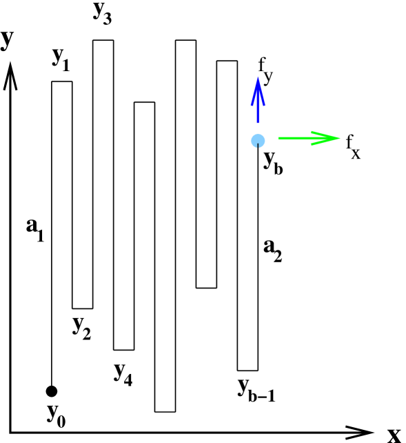
The phase boundary between the collapsed and the extended phase can be obtained by calculating the macroscopic shape of the collapsed phase at low temperatures. Let , and , where is the temperature. We set the Boltzmann constant equal to . The energy of the configuration which mimics the -sheet is (see Fig. 1)
| (2) |
where, as illustrated in Fig. 1, is the height (number of steps in the -direction) of the first column, is the height of the last column and is the number of steps in the -direction.
Following the approach developed in suppl , we express the sum appearing in Eq. (2) as a surface tension term. The macroscopic shape of the polymer is calculated and the value of at which the collapsed phase becomes unstable gives the critical value, , in terms of and :
| (3) |
Eq. (3) gives the complete three dimensional phase boundary. For () Eq. (3) reduces to the following simple expression for the critical force when pulling along the -direction
| (4) |
This coincides with the result obtained by transfer matrix methods rosa . However, that method is not easily generalized to the case where force is applied along the -direction. Eq. (3), on the other hand, is sufficiently general to yield an expression for the critical force when pulling along the -direction. Setting (or ) yields the critical force when pulling along the -axis:
| (5) |
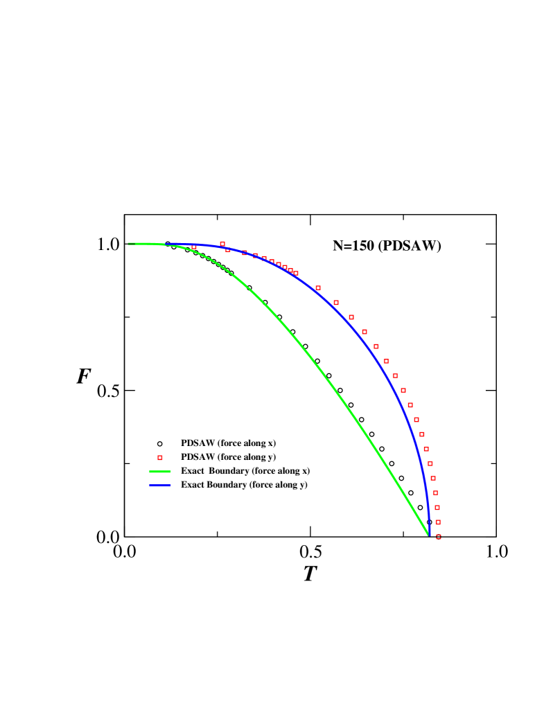
For zero force (i.e. ) the expression reduces to the exact value ( if we set ) at which thermal unfolding occurs. The exact phase boundaries obtained from Eqs. (4) and (5) are shown in Fig. 2 and compared to numerical results obtained for .


III Numerical Analysis
Our numerical studies of the process of force induced protein unfolding are based on the exact enumeration of all possible conformations of the chain. This approach not only enables us to obtain precise estimates for the phase boundary, but also allows us to study the intermediate states crucial to events occurring during the mechanical stretching process altmann ; rief1 ; schwaiger . In this study we have combined the power of parallel processing and transfer matrix calculations to extend the limit of earlier studies not just by one or two monomers but five times over! Thus we have extended from the previous longest chain length kumar to much longer chains of up to steps. The partition function is
| (6) |
where is the total number of -stepped PDSAWs having non-bonded nearest neighbor pairs with end-to-end vector .
The value of the transition temperature (for fixed force and finite ) can be obtained from the fluctuations in the number of non-bonded nearest neighbor interactions. The fluctuations are defined as , with the ’th moment given by
| (7) |
When the fluctuations are plotted as a function of temperature the resulting graph (Fig. 3a) has a peak at the transition temperature. The inset shows that the height of the peak in the fluctuation curve grows as a power-law with , this being the hall mark of a phase transition. By setting we obtain (for ) at zero force () the transition temperature . This is already quite close to the value obtained in the thermodynamic limit (). The bottom panel in Fig. 3 shows the variation in the transition temperature plotted against and we see a pronounced curvature for large making an extrapolation to the limit very difficult.
In Fig. 2 we show the force-temperature diagrams for when pulling along the - and -axis (circles and squares, respectively). These numerical estimates for the phase-boundary are in excellent agreement with the analytical results (shown as solid lines) obtained from Eqs. (4) and (5). Thus exact enumeration technique works quite well even for small as far as the phase diagram is concerned. This has also been seen earlier mishra in case of the surface adsorption.
III.1 Constant Force and Constant Distance Ensembles
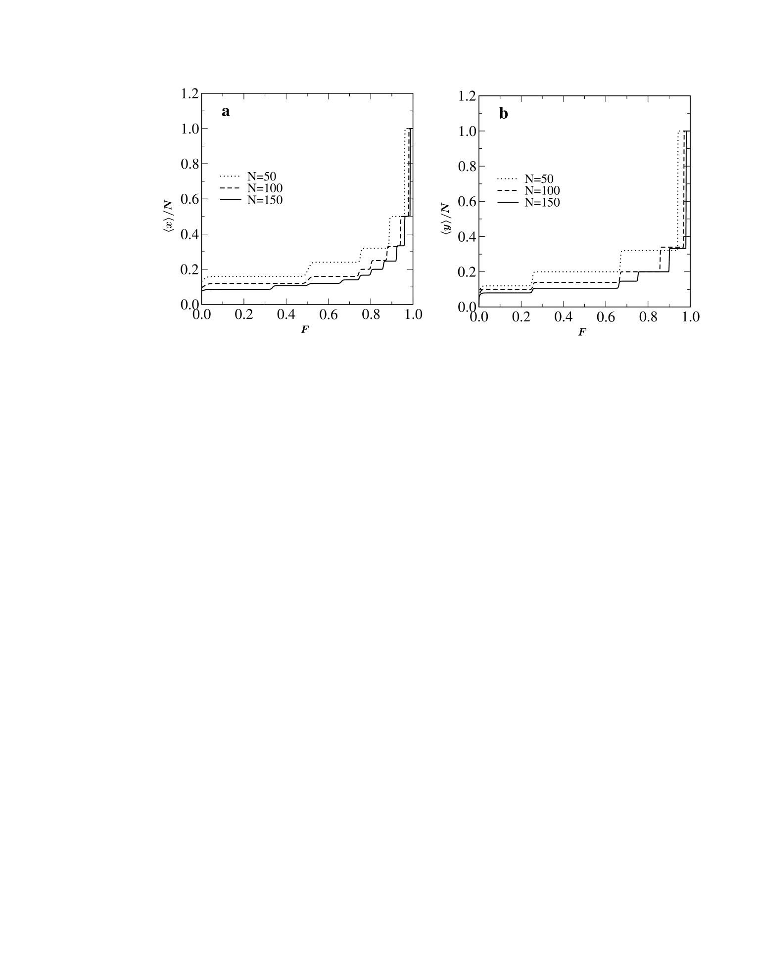
Many biological reactions involve large conformational changes providing a well defined mechanical reaction co-ordinate (e.g. the end-to-end distance of a bio-polymer), which has been used in force spectroscopy experiments to follow the progress of the reaction rief ; carrion1 . Within the constant force ensemble (CFE) the theoretical predictions based on exact enumeration results provide qualitative description of the outcomes of such experiments kumar ; kumar1 (like the existence of intermediate states and different pathways to unfolding). In Fig. 4 we have plotted the average extension as a function of the applied force. Fig. 4a shows the result when the force is applied in the -direction and Fig. 4b when the force is applied in the -direction. In both cases we see the existence of several plateaus showing that there are many intermediate states between the collapsed and fully extended state. A major difference is that the number of these intermediate states seems to grow much faster with the chain length when pulling in the -direction as compared to pulling in the -direction.

The appearance of the plateaus in the force-extension curves as well as the differences between the two cases have a simple heuristic explanation. At very low temperature there are no entropic contributions to the free energy which is thus dominated by the energetic terms arising from nearest-neighbor interactions and the applied force. When pulling in the -direction we have to maximize the quantity , where is the number of contacts. For this means just maximizing , and this is achieved by zigzag conformations inscribed in a rectangle which is as close to a square as possible so that is close to . As the force is increased other configurations may become energetically favored, essentially corresponding to decreasing the width of the rectangle by a unit and increasing the length correspondingly (a more detailed explanation can be found in Guttmann08 ; see also Krawczyk05 ). So the plateaus seen in Fig. 4a arise from inscribing a PDSAW of fixed length in rectangles, going from right to left, of width as evidenced by the fact that these plateaus have height . The types of conformations giving rise to the right-most plateaus are represented schematically in Figs. 5a-c. When pulling in the -direction we again get a competition between the force which tends to maximize the distance of the end-point in the -direction and interactions which try to inscribe the PDSAW into a square. As illustrated in Figs. 5d-f the conformations giving rise to the right-most plateaus are now those where the PDSAW is inscribed in a rectangle of length . This can be seen in Fig. 4b where these plateaus have height . Even lengths cannot occur because for these the end-point would have a -component close to 0 giving only a small energetic contribution from the applied force. The upshot is that for a given length the number of plateaus when pulling in the -direction will be about twice the number of plateaus when pulling in the -direction.
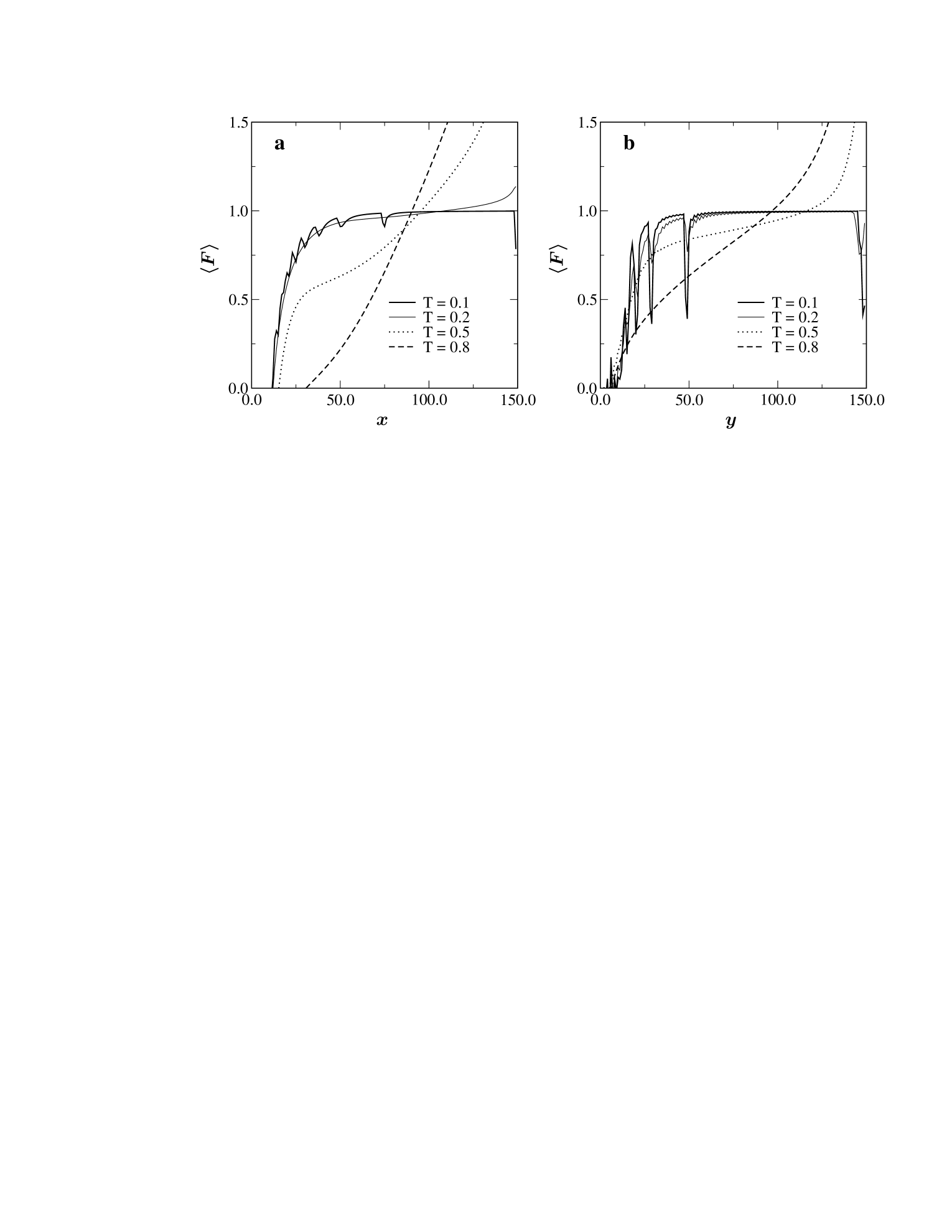
Our longer series data also allows us to go a step further in analyzing the model in the constant distance ensemble (CDE). This is the ensemble best suited to the analysis of experiments performed using apparatus such as atomic force microscopes. In Fig. 6 we have plotted the average force kumar1 as a function of the extension when pulling in either the - or -direction. Striking differences between the two cases are obvious from these plots. Most obviously we note that at the low temperature the force extension curve obtained for pulling in the -direction shows unzipping like transition characterized by having smooth plateaus. However, when the chain is being pulled in the -direction (at the same temperature), the force extension curve exhibits “saw-tooth” like oscillations indicating that the transition is akin to shearing. This clearly demonstrates that even the nature of the unfolding transition can change dramatically solely by varying the pulling direction.
IV Anisotropic-Self-Attracting-Self-Avoiding Walks
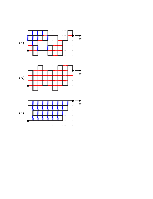
The model described above has an exact solution and gives qualitative features similar to experiments. However, the physical constraints imposed by experimental set-ups has not been taken fully into account. For example, in experiments using atomic force microscopes, receptor and ligand molecules are attached to a substrate and a transducer, respectively, which introduce anisotropy in the systems. Also steric constraints due to the confinement imposed by the experimental set-up can lead to a loss of entropy and thus result in modifications to the behavior of the chain. Furthermore the constraint of partially directing the walk so it cannot take steps in the negative -direction is not really appropriate to most experimental conditions. Such a constraint is typically only appropriate when the system is under flow or constant external field lemak ; lemak1 . A more realistic model of polymers is provided by self-attracting-self avoiding walks (SASAWs), which is well suited to the modeling of a linear chain in a poor solvent degennes ; vander . However, this model is isotropic in nature. In this paper we introduce anisotropy to the model. We achieve this by considering nearest neighbor interactions with different strengths along the - and -directions as shown in Fig. 7a. This is in accordance with real proteins where the interactions along different directions can differ by orders of magnitude creighton . Hence by changing the strength of the interactions one can vary the degree of anisotropy in the system and study the effect this has on the force-temperature phase diagram. The partition function for anisotropic-self-attracting-self-avoiding walks (ASASAWs) may be written as
| (8) |
Here is the total number of ASASAWs of steps having and nearest neighbor pairs along the - and -directions, respectively, while () are the Boltzmann weights associated with the nearest neighbor interactions between non-bonded monomers along, respectively, the - and -directions.
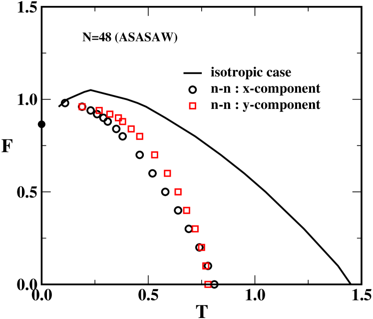
The qualitative as well as quantitative features of the force-temperature phase diagram as shown in Fig. 8 for the isotropic case (i.e. ) remain the same as those reported in kumar1 . To make our model closely resemble the PDSAW discussed above, we set either or and apply a force along the -direction. For the ground state is dominated by configurations similar to the one shown in Fig. 7(b). This closely resembles the PDSAW model (Fig. 1) subjected to a force along the -axis and the nature of the transition is akin to an unzipping transition. On the other hand for the ground state is dominated by configurations like the one shown in Fig. 7(c). This closely resembles the configurations of Fig. 1 with a force along the -axis and consequently the nature of the transition is akin to a shearing type transition. It should be noted that the number of ASASAWs, , is different from the number of PDSAWs even if we put . We observe a significant decrease in the transition temperature compared to SASAWs. This is caused by a decrease in entropy which allows the polymer to acquire conformations similar to a -sheet. The effect of surface confinement is also evident from these plots. The transition temperature is found to be less for in comparison to . Another major difference between the ASASAW and SASAW phase-diagrams is that there appears to be no re-entrance in the ASASAW model when or . It is well known that the re-entrant behavior of the SASAW model is due to a non-zero ground state entropy, that is, the number of configurations in the ground state grow exponentially with (these configurations are just Hamiltonian walks inscribed in a rectangle with side lengths as close as possible to ). For the ASASAWs we study here the ground-states are, as argued above, folded sheets as in Fig.7(b) and (c), respectively. The number of such configurations do not grow exponentially with and are thus too few to give a non-zero ground state entropy, which is why we do not see re-entrance. However, if both and are greater than 1 then one may see a re-entrant phase diagram.
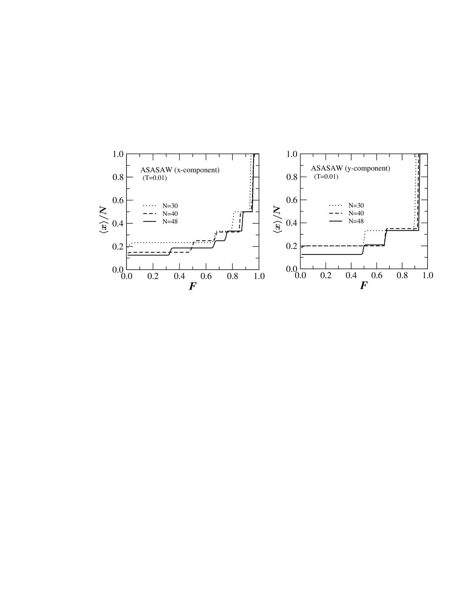
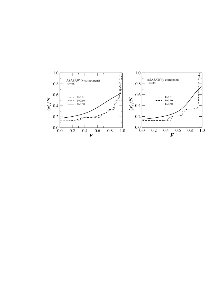
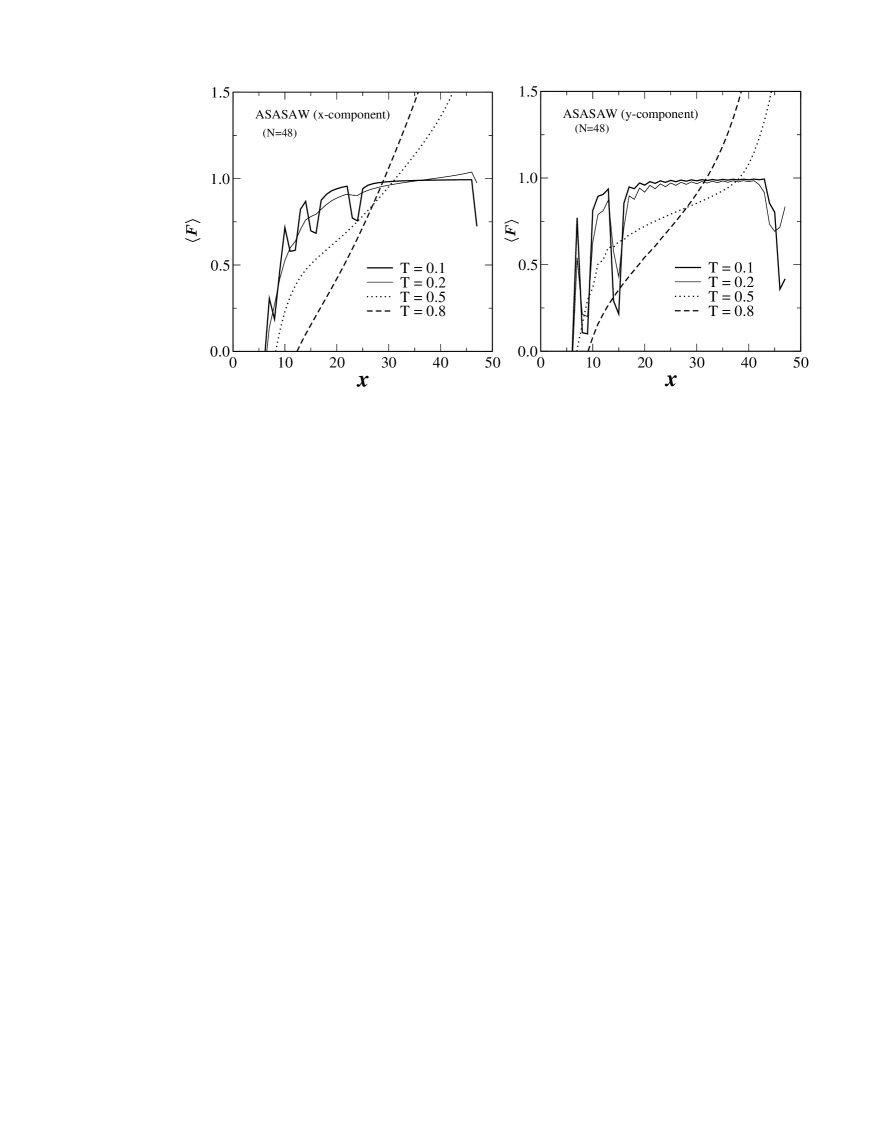
The force extension curve shown in Fig. 9 not only shows the existence of intermediate states but also the emergence of new states depending on the direction of the interactions in accordance with the findings for PDSAWs. As the temperature is increased we observe in Fig. 10 (as expected) that the intermediate states are washed out due to the resulting increase in entropy. We also observe that the system attains a higher stability against the force when the interactions are along the -direction and that intermediate states survive even at high temperatures as may be seen from Fig. 10.
Finally we analyze the ASASAW model in the constant distance ensemble. In Fig. 11 we have plotted the average force kumar1 as a function of the extension when pulling in the -direction with interactions either along the - or -direction. The results are qualitatively very similar to those obtained for the PDSAW model (see Fig. 6). In particular we note that the oscillation at low-temperature are much more pronounced in the case where the interactions are in the -direction. As explained above (see Fig. 7) there is a close correspondence between the ground-state (low-temperature) configurations of the ASASAW with interactions in the - or -directions and the PDSAW with a force applied along the - or -direction, respectively. This close correspondence is reflected in the similarity of the results.
V Conclusion
In summary we have demonstrated via the analytical solution for the phase boundary of PDSAWs as well as through high precision numerical calculations that changing the pulling direction can change the nature of the unfolding transitions and give rise to very different phase diagrams. The emergence of many new intermediate states suggests that there may be many pathways to the unfolding of a polymer. The findings for the PDSAW model have been confirmed by our study of ASASAWs. The inclusion of anisotropy in the traditional SASAW model of polymers gives unequivocal evidence that the features observed here for the PDSAW model are in fact generally true and not an artifact of the PDSAW model. In future additional work like extensive Monte Carlo simulations and molecular dynamics studies are needed to better understand the role played by anisotropy and how varying the pulling direction can help us gain a better and deeper understanding of biomolecules.
Acknowledgments
This research has been supported by the Department of Science and Technology and University Grants Commissions, India and also by the Australian Research Council. The calculations presented in this paper used the computational resources of the Australian Partnership for Advanced Computing (APAC) and the Victorian Partnership for Advanced Computing (VPAC).
References
- (1) M. Rief et al, Science 276, 1109 (1997).
- (2) M. S. Z. Kellermayer, S. B. Smith, H. L. Granzier and C. Bustamante, Science 276, 1112 (1997).
- (3) L. Tskhovrebova, J. Trinick, J. A. Sleep, and R. M. Simmons, Nature 387, 308 (1997).
- (4) C. Bustamante, Y. R. Chemla, N. R. Forde and D. Izhaky, Annu. Rev. Biochem. 73, 705 (2004).
- (5) M. Carrion-Vazquez et al, PNAS 96, 3694 (1999).
- (6) L. Serrano et al, J. Mol. Biol. 224, 783 (1992).
- (7) A. E. Eriksson et al, Science 255, 178 (1992).
- (8) D. J. Brockwell et al, Nat. Struct. Biol. 10, 731 (2003).
- (9) M. Carrion-Vazquez et al, Nat. Struct. Biol. 10, 738 (2003).
- (10) M. Kouza, C. K. Hu, and M. S. Li, J. Chem. Phys. 128, 045103 (2008).
- (11) A. Matouschek and C. Bustamante, Nat. Struct. Biol. 10, 674 (2003).
- (12) H. Dietz and M. Rief, PNAS 103, 1244 (2006).
- (13) H. Dietz, F. Berkemeier, M. Bertz and M. Rief, PNAS 103, 12724 (2006).
- (14) M. Fixman, J. Chem. Phys. 58, 1559 (1973).
- (15) M. Doi and S. F. Edwards, Theory of Polymer Dynamics, (Oxford Univ. Press, Oxford, 1988).
- (16) J. F. Marko and E. D. Siggia, Macromolecules 28, 8759 (1995).
- (17) M. Rief, J. M. Fernandez and H. E. Gaub, Phys. Rev. Lett. 81, 4764 (1998).
- (18) P. G. de Gennes, Scaling Concepts in Polymer Physics, (Cornell Univ. Press, Ithaca, 1979).
- (19) T. E. Creighton, Protein Folding, (W. H. Freemann, New York, 1992).
- (20) A. Rosa, D. Marenduzzo, A. Maritan and F. Seno, Phys. Rev. E 67, 041802 (2003).
- (21) S. Kumar and D. Giri, Phys. Rev. Lett. 98, 048101 (2007)
- (22) C. Vanderzande, Lattice Models of Polymers, (Cambridge Univ. Press, Cambridge, 1998); S. Kumar and Y. Singh, Phys. Rev. A42, 7151 (1990).
- (23) The full details of the calculations will be given elsewhere.
- (24) S. M. Altmann et al, Structure 10, 1085 (2002).
- (25) H. Dietz and M. Rief, PNAS 101, 16192 (2004).
- (26) I. Schwaiger et al, Nat. Struc. Mol. Bio. 11, 81 (2004).
- (27) P. K. Mishra, S. Kumar and Y. Singh, Physica A 323, 453 (2003).
- (28) S. Kumar, I. Jensen, J. L. Jacobsen and A. J. Guttmann, Phys. Rev. Lett. 98, 128101 (2007).
- (29) A. J. Guttmann, J. L. Jacobsen, I. Jensen and S. Kumar, J. Math. Chem. (DOI: 10.1007/s10910-008-9377-4). Preprint arXiv:0711.3482
- (30) J. Krawczyk, A. L. Owczarek, T. Prellberg and A. Rechnitzer, Europhys. Lett. 70, 726 (2005).
- (31) A. S. Lemak, J. R. Lepock and J. Z. Y. Chen, Phys. Rev. E 67, 031910 (2003).
- (32) A. S. Lemak, J. R. Lepock and J. Z. Y. Chen, Proteins: Structures, Function and Genetics 51, 224 (2003).