Routine monitoring and analysis of ocean swell fields using a spaceborne SAR
Abstract
Satellite Synthetic Aperture Radar (SAR) observations can provide a global view of ocean swell fields when using a specific ”wave mode” sampling. A methodology is presented to routinely derive integral properties of the longer wavelength (swell) portion of the wave spectrum from SAR Level 2 products, and both monitor and predict their evolution across ocean basins. SAR-derived estimates of swell height, and energy-weighted peak period and direction, are validated against buoy observations, and the peak directions are used to project the peak periods in one dimension along the corresponding great circle route, both forward and back in time, using the peak period group velocity. The resulting real time dataset of great circle-projected peak periods produces two-dimensional maps that can be used to monitor and predict the spatial extent, and temporal evolution, of individual ocean swell fields as they propagate from their source region to distant coastlines. The methodology is found to be consistent with the dispersive arrival of peak swell periods at a mid-ocean buoy. The simple great circle propagation method cannot project the swell heights in space like the peak periods, because energy evolution along a great circle is a function of the source storm characteristics and the unknown swell dissipation rate. A more general geometric optics model is thus proposed for the far field of the storms. This model is applied here to determine the attenuation over long distances. For one of the largest recorded storms, observations of 15 s period swells are consistent with a constant dissipation rate that corresponds to a 3300 km e-folding scale for the energy. In this case, swell dissipation is a significant term in the wave energy balance at global scales.
COLLARD ET AL. \titlerunningheadOBSERVING OCEAN SWELL FIELDS \authoraddrFabrice Collard, Collecte Localisation Satellites, division Radar, 29280 Plouzané, France. (Dr.fab@cls.fr) \authoraddrFabrice Ardhuin, Service Hydrographique et Océanographique de la Marine, 29609 Brest, France. (ardhuin@shom.fr) \authoraddrBertrand Chapron, Ifremer, Laboratoire d’Océanographie Spatiale, Centre de Brest, 29280 Plouzané, France. (bertrand.chapron@ifremer.fr)
1 Introduction
Storms over the ocean produce long surface gravity waves that propagate as swell out of their generation area. In deep water, the wave phase speed and period are proportional. As the phase speed of the dominant waves does not exceed 1.2 times the wind speed at 10 m height (Pierson and Moskowitz, 1964), the longest period waves must be generated by very intense winds. For example, the generation of waves of period larger than 16 s requires winds with speeds over 18 m s-1 blowing over a distance of the order of 1000 km, to produce a significant energy, or yet stronger winds over a shorter fetch (Munk et al., 1963). Such a large region of high winds is generally associated with a smaller storm center from which the long swells radiate. Waves further evolve after their generation with an important transfer of energy towards both high and low frequencies, due to nonlinear wave-wave interactions. Away from that core, nonlinear interactions become negligible (Hasselmann, 1963) and long period swells have been observed to propagate over very large distances, up to half-way around the globe (Munk et al., 1963), radiating a large amount of momentum and energy across ocean basins. This measurable long-distance propagation is made possible by a limited loss of energy.
The wave field at any time , latitude and longitude , is described by its spectral densities as a function of frequency and direction . In the limit of geometrical optics, the spectral density is radiated at the group speed in the direction of wave propagation, and can be expressed as a function of at any previous time . Allowing for a spatial decay at a rate , the spectral energy balance is (e.g. Munk et al., 1963)
| (1) |
In deep water without current, the initial position , and direction are given by following the great circle that goes through the point of coordinates with a direction over a distance . This corresponds to a spherical distance along the great circle, where is the Earth radius.
Equation (1) can be used to invert from wave measurements. For swell periods shorter than 13 s, Snodgrass et al. (1966) have measured an e-folding scale km (this number corresponds to a 0.1 dB/degree attenuation in their analysis). For larger periods, Snodgrass et al. (1966) could only conclude that is larger, possibly infinite. In the past 40 years, little progress has been made on these conclusions (WISE Group, 2007). Yet this question if of high practical importance, either for wave forecasting (e.g. Rascle et al., 2008) or other geophysical investigations regarding air-sea fluxes or microseismic noise (e.g. Grachev and Fairall, 2001; Kedar et al., 2008).
A theoretical upper bound for is given by the viscous theory (Dore, 1978, see also Appendix A for a simple derivation). According to theory, the largest shears are found right above the water surface, and the air viscosity dominates the dissipation of swells, giving, in deep water,
| (2) |
where is the air viscosity, . For s this gives km, which means that over a realistic propagation distance of 10000 km the energy of 13 s swells is only reduced by 25%.
Swells are thus expected to be very consistent over distances that are only limited by the size of ocean basins. The analysis of swells at this global scale should provide insights into their dynamics, including propagation and dissipation, but also into the structure of the generating areas, in a way similar to the use of the cosmic microwave background for the analysis of the early universe.
The present paper provides two important intermediate steps toward that goal. First, we demonstrate in section 2 how sparse data from a single space-borne synthetic aperture radar can be combined dynamically to provide a consistent picture of swell fields. This internal consistency reveals the quality of the SAR-derived dataset which we further verify quantitatively with buoy data. In section 3, we discuss and derive the asymptotic far-field swell energy evolution. Numerical investigations are performed to check the validity of the asymptotic solutions. This result provides a tool to interpret measured swell heights in terms of propagation and dissipation. This method is illustrated with one example that corresponds to a strong swell dissipation. Conclusions follow in section 4.
2 Space-time consistency of space-borne swell observations
Investigations by Holt et al. (1998) and Heimbach and Hasselmann (2000) have shown that space-borne synthetic aperture radar (SAR) data can be used to image the same swell field over 3 to 10 days as it propagates along the ocean surface. These preliminary studies have shown that the combination of SAR data at different places and times yields a position of the generating storm, and predictions for the arrival time of swells with different periods and directions. Heimbach and Hasselmann (2000) have further pointed to shortcomings in the wind provided by an atmospheric circulation model for a given Southern Ocean storm, based on systematic biases in wind-forced wave model results compared to SAR observations. Unfortunately, the systematic analysis of such data has been very limited, and generally confined to data assimilation in wave forecasting models [e.g. Hasselmann et al. 1997; Breivik et al. 1998; Aouf et al. 2006]. This narrow use of SAR data is due to three essential difficulties.
First, a SAR image is not a picture of the ocean surface and the relationship between the spectrum of the SAR image and that of the ocean surface elevation is nonlinear and fairly complex (e.g. Krogstad, 1992). Sophisticated methods have been developed in order to estimate the surface elevation spectrum (e.g. Hasselmann et al., 1996; Schulz-Stellenfleth et al., 2005). These methods had to be implemented by the user of the data, and generally required some a priori first guess of the wave field provided by a numerical model. For longer wave systems, the imaging mechanisms are essentially quasi-linear, making possible a simpler methodology used by the European Space Agency (ESA) to generate a level 2 (L2) product. The method is fully described by Chapron et al. (2001). It uses no outside wave information, and builds on the use of complex SAR data developed by Engen and Johnsen (1995) to remove the 180∘ directional ambiguity in wave propagation direction. The quality of the L2 data has been repeatedly analyzed (e.g. Johnsen et al., 2006; Collard et al., 2005). Because long ocean swells have large wavelengths and smaller steepnesses, the L2 products corresponding to this spectral range have higher relative quality, confirming that the imaging mechanism is well described under the quasi-linear assumption.
All SAR data used here are such L2 products, provided by ESA and obtained with the L2 processor version operational since November 2007, and described by Johnsen and Collard (2004). The data for times before that date were reprocessed with this same processor. In previous real-time data, frequent low wavenumber artefacts were caused by insufficient filtering of non-wave signatures in the radar images. This filtering is necessary to remove the contributions of atmospheric patterns or other surface phenomena like ships, slicks, sea ice, or islands, with spectral signatures that can overlap the swell spectra. The L2 product contains directional wave spectra with a resolution of 10∘ in directions and an exponential discretization in wavenumbers spanning wavelengths of 30 to 800 m with 24 exponentially spaced wavenumbers, corresponding to wave periods with a 7% increment from one to the next.
The second practical problem is that the data obtained from an orbiting platform are sparse and with a sampling that makes a direct analysis difficult. Hereafter, we show that the space-time consistency of the swell field can be used to fill in the gaps in the observations and produce continuous observations of swell periods and directions in space and time.
Third, and last, for a simple use of SAR data, some parameters that are not affected by the variable resolution is SAR scenes (Kerbaol et al., 1998). Schulz-Stellenfleth et al. (2007) have proposed to produce parameters representing the entire sea state by extending the resolved spectrum with an empirical windsa contribution. Here we take the opposite approach and restrict the resolved part of the spectrum by using a spectral partitioning (see Appendix B for details) to retrieve the swell significant wave height , defined as four times the square root of the energy of one swell system, and the peak period and peak directions . Thus one SAR typically produced one or two swell parameters for distinct swell systems.
For , only very limited validations have been performed (Collard et al., 2006). We thus perform a thorough analysis of SAR-derived comparing to co-located buoy data (see Appendix B for details).
The bias on derived from ESA Level 2 products is found to be primarily a function of the swell height and wind speed, increasing with height and decreasing with wind speed. Variations in standard deviation are dominated by the swell height and peak period, with the most accurate estimations for intermediate periods of 14 to 17 s.For wind speeds in the range 3 to 8 m s-1, has a bias of 0.24 m and the standard deviation of the errors is 0.29 m.
We thus corrected the values of by subtracting a bias model given by
| (3) |
where is in meters and the wind speed is in m s-1. From now on, all the reported values of will be corrected using this expression. After correction, the standard deviation of estimates is reduced to less than
| (4) |
where and are in meters.
The quality of and has already been carefully studied and are routinely monitored. The root mean square (r.m.s.) error on is less than 10% of the measured value for s, and the r.m.s. error on is 22∘ for these same swells (Johnsen and Collard, 2004), with little bias. Because few directional in situ measurements are available, we demonstrate here an original semi-quantitative dynamical validation of these two parameters.
2.1 Virtual wave observers
Given these SAR-derived estimates of and , linear dispersion relationship and the principle of geometrical optics can then be exploited to predict arrival times and locations of the swell.
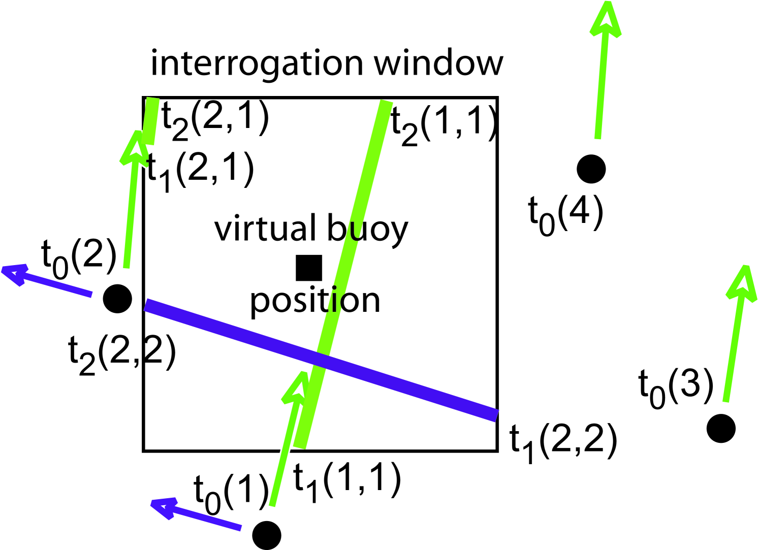
In order to obtain swell conditions at the location of a ”virtual wave observer”, we define an interrogation window covering 2 by 2 degrees in latitude and longitude. According to the SAR-derived peak parameters, swell partitions from the entire ocean basin are propagated, both forward and backward, along great circles in space and time. These theoretical trajectories are followed with a constant group speed , starting off in direction from the observation point. From any observation time , these great circles may cut through the interrogation window from times to (thick solid lines in figure 1, with different colors for different partitions). As the maximum value of and is increased from 6 hours to 6 days, the time-evolution of the peak frequencies and peak directions at the virtual observer gradually reveals similar ridges to the one observed in real buoy measurements (figure 2).
In fig. 2b-d, each horizontal colored segment corresponds to one swell partition that crosses the spatial window between times and . Some segments are very short, corresponding to trajectories that barely cut one corner of the window.
Clearly the SAR detects the direction of the most energetic part of the wave spectrum measured by the buoys (fig. 2a). At frequencies above 0.1Hz, the virtual observer patterns appear rather noisy. Shorter scales are not so correlated. These shorter components are often observed as part of the wind sea for which the propagation with a single group speed and direction is not a good approximation. Also, propagated high frequency swells, such as the 0.12 Hz waves coming from direction 200 on July 10, do not show up in the real buoy record. This is possibly the result of a relatively high dissipation rate for these swells.
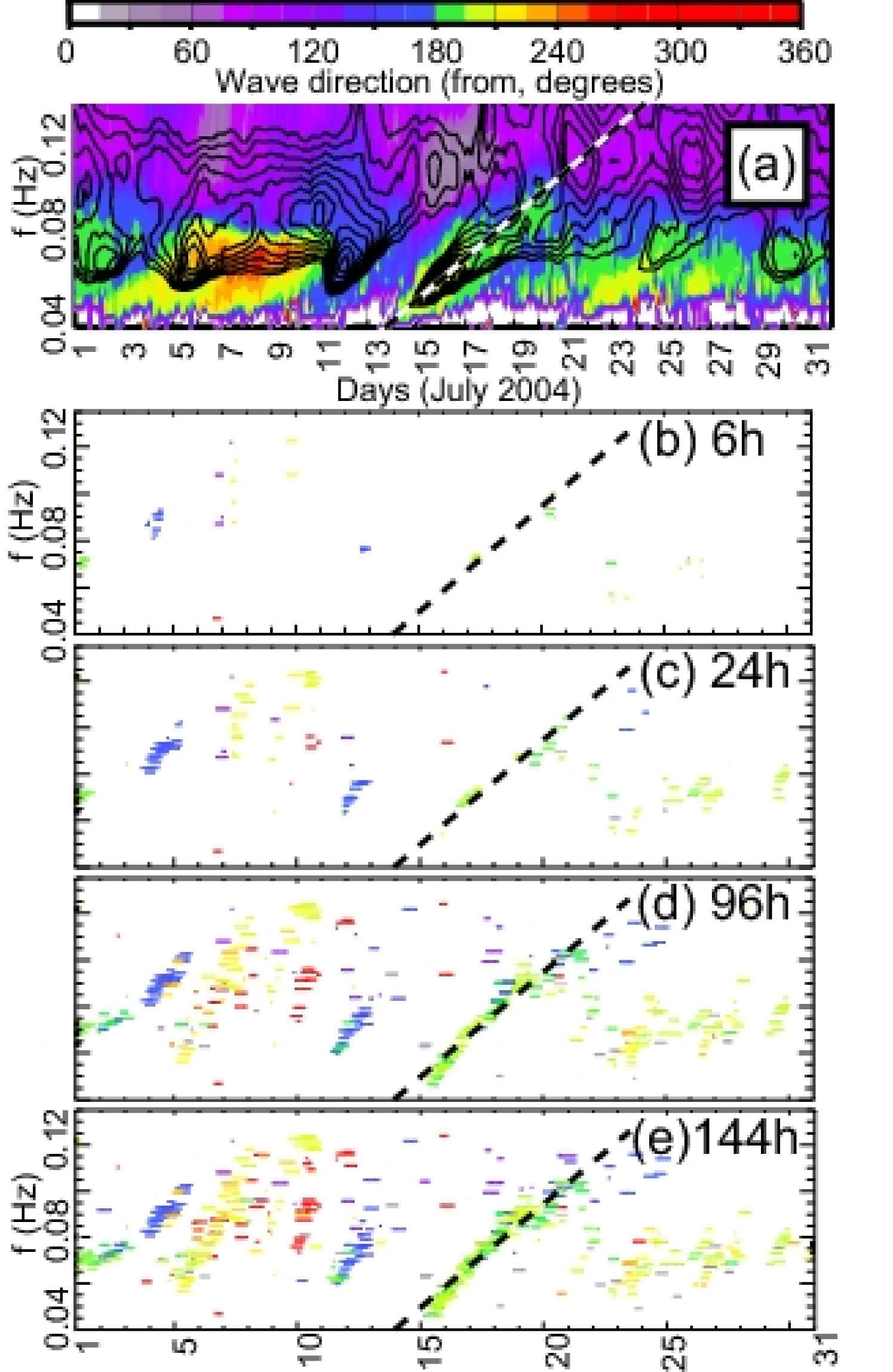
For frequencies below 0.08 Hz, the virtual observer shows ridge-like structures similar to those observed in situ due to the dispersive arrivals of swells from remote storms (e.g. Munk et al., 1963; Gjevik et al., 1988). Even the faintest events are well detected, such as the 0.06 Hz arrival on 23 July, even though that 15 s swell of 0.5 m is dwarfed by a another 0.8 m and 12 s swell, and a 2 m and 8 s wind sea. Swell detection with the virtual observer reaches its limits when the swell height is very low, such as on 3 July with a 20 s 0.3 m swell well detected by the buoy (the green-orange ridge at 0.05 Hz). Because we use a single trajectory emanating from one observed swell partition the relatively small interrogation window can easily be missed after 10000 km of propagation.
Our discrete propagation technique suffers from a randomized version of the “garden sprinkler effect” that, if not corrected for, can create unrealistic flower-like patterns in the far field of storms in numerical wave models that use a discretized spectrum (e.g. Tolman, 2002). Our choice of a single group speed and direction, because a narrow swell spectrum is not resolved by the SAR, produces a discrete wave field (the dots in figure 3). With the present processing this is smoothed by the finite size of our interrogation window (figure 1). An extension of the present technique could use neighboring group speeds and directions to take into account the frequency and directional spread of the sea state, which would allow the use of a smaller window. Just like the estimation of propagated wave heights, discussed below, the estimation of a spectra width that cannot be resolved by the SAR may use some further information on the structure of the generating storm.
Other errors in the present technique can also be attributed to the SAR processing. In particular, a maximum value is defined for the transfer function used to obtain the wave spectrum from the SAR image (Johnsen and Collard, 2004). Although this is designed to prevent the amplification of measurement noise, long swells such as this 20 s event have very small slopes, and it is likely that they are underestimated in the wave spectrum due to this threshold in the processing.
When propagated for 6 days, without any other information than the peak frequency and direction at the time of observations, the waves are remarkably consistent with the latest local observations. For the southern swells arriving at Christmas Island between July 16 and 21 (figure 2), the difference in arrival times given by the virtual oberver and real buoy is typically less than 12 h. This is less than 10% of the maximum time between the SAR observation and the virtual observer record. This implies that the accuracy of the peak period estimate for each SAR partition must also be less than 10%, consistent with previous validation studies (Johnsen and Collard, 2004; Johnsen et al., 2006). The consistency of the arrival directions along the ridges also suggests that the root mean square (RMS) error in peak direction estimates must be close to 20∘, comparable to the 22∘ RMS difference between mean wave directions obtained from SAR wave mode and a numerical wave model for waves with periods longer than 12 s (Johnsen and Collard, 2004).
Although it cannot replace the spectral resolving power of a buoy, the performance of the virtual observer is therefore comparable or better to that of human observers in terms of peak period and direction (Munk and Traylor, 1947). The really missing bit is a wave height estimate along the swell propagation path. We will show that this may be obtained by estimating the source storm characteristics and the dissipation rate of swell energy.
2.2 Storm source identification and ”fireworks”
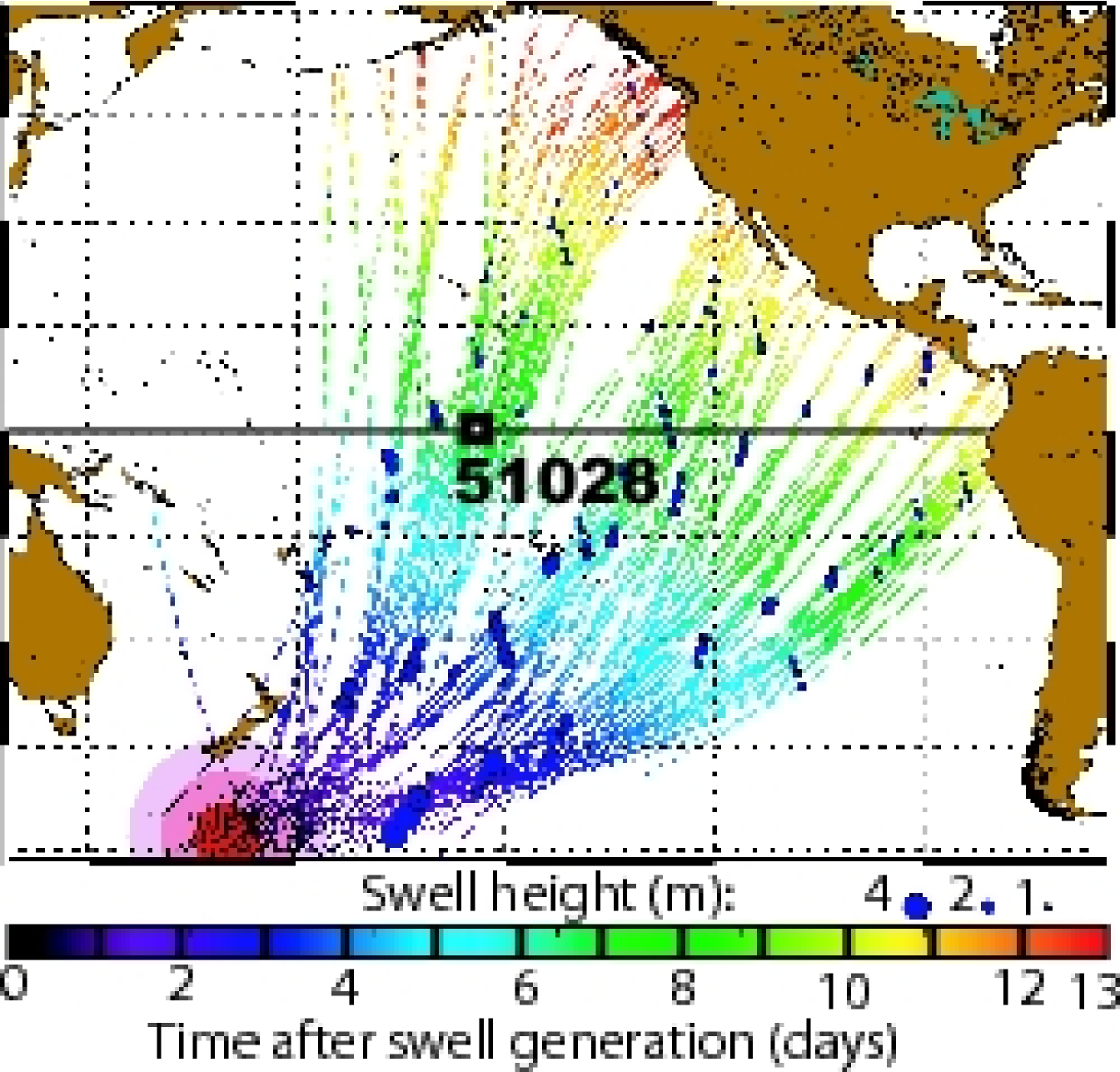
Along the estimated trajectories, virtual observations can further be produced in a similar fashion. The animation of these propagated swells confirms the very well organized nature of storm swells crossing large ocean basins.
From the relatively sparse and
track-based initial satellite observation sampling, the swell
persistency can then be used to capture ”fireworks” patterns
exploding from the few intense storms that occur over a period of
several days (see figure 3 and auxiliary
animation). In large ocean basins where swells are likely to be
imaged several times by the same satellite, these fireworks can be
used to estimate the time of arrival of swells from any given
storm (e.g. Holt et al., 1998). For this reason, these
animations have been produced routinely every day since August
2007, for the Pacific, Indian, and Atlantic oceans (see
http://www.boost-technologies.com/esa/images/, e.g.
nrt_pac.gif for the Pacific Ocean).
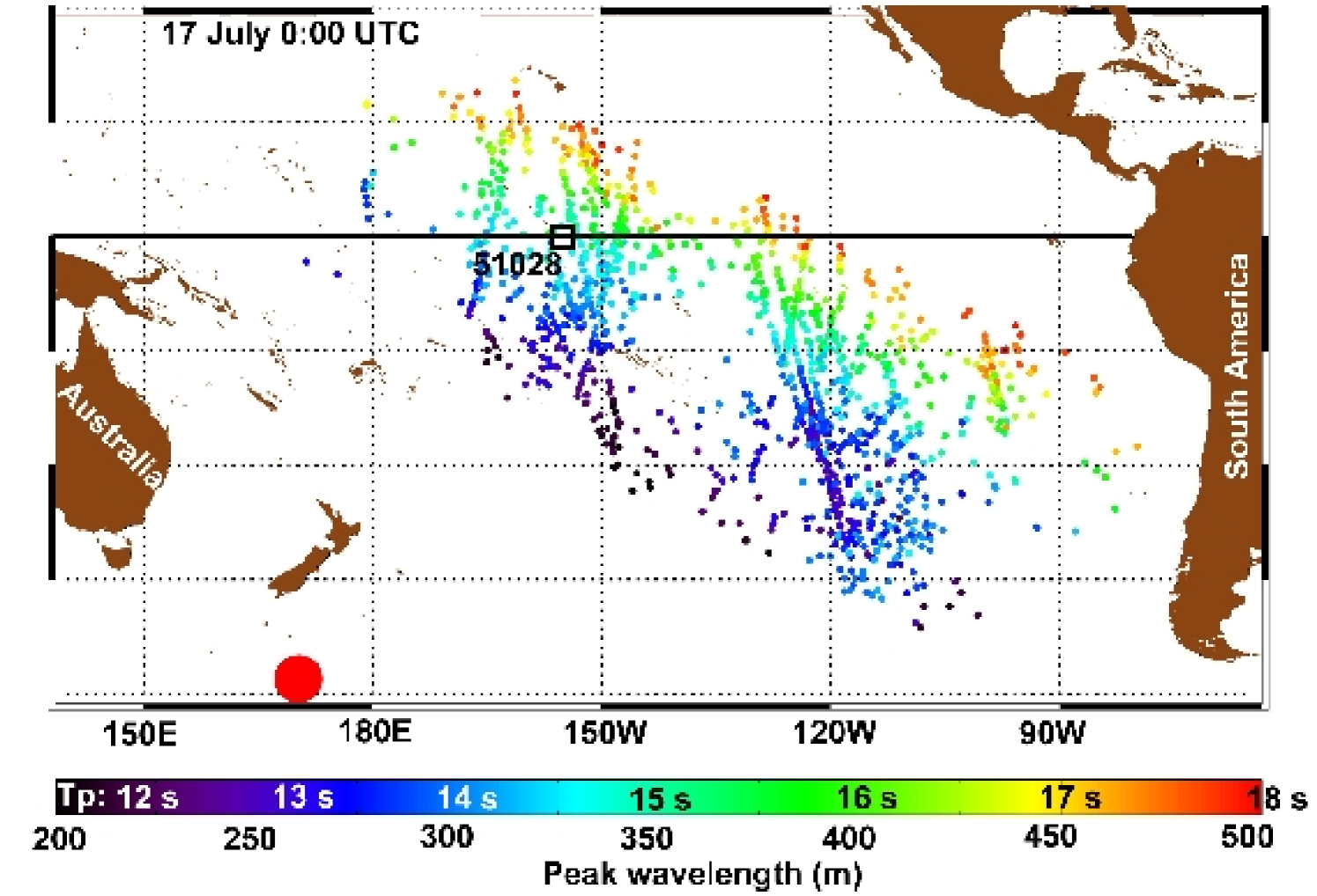
Using backward trajectories, the location and date of swell sources can further be defined as the spatial and temporal center of the convergence area and time of the trajectories. These positions have been verified to correspond to high wind conditions observed by scatterometers and reproduced by ECMWF wind analyses. We consider these storms to be the source of all the swell partitions that produce trajectories that pass within 12 hours and 2000 km of their center. This processing, similar to the one performed by Heimbach and Hasselmann (2000), provides a global view of swell fields in both space and time, extending the coverage of similar techniques based on buoy data (Hanson and Phillips, 2001). In figure 4, a swell covers one Earth quadrant away from the storm, with a large detection gap that extends from the Southern Pacific to California. This blank area is the long shadow cast by French Polynesia where wave energy is dissipated in the surf (e.g. Munk et al., 1963). Observations were restricted to swell partitions with periods close to 17 s, but the full dataset typically covers swells with periods of 12 to 18 s, as shown in figure 3.
The apparent self-consistency of both the virtual buoy plot (figure 2.d) and the fireworks animations, are the result of the large auto-correlation length of the swell fields, which was expected from the in situ measurements of Darbyshire (1958); Munk et al. (1963); Snodgrass et al. (1966). Yet, these plots could not exhibit such patterns without a good accuracy of the SAR-derived peak periods and directions, used in the propagation methodology.
3 Far-field swell energy
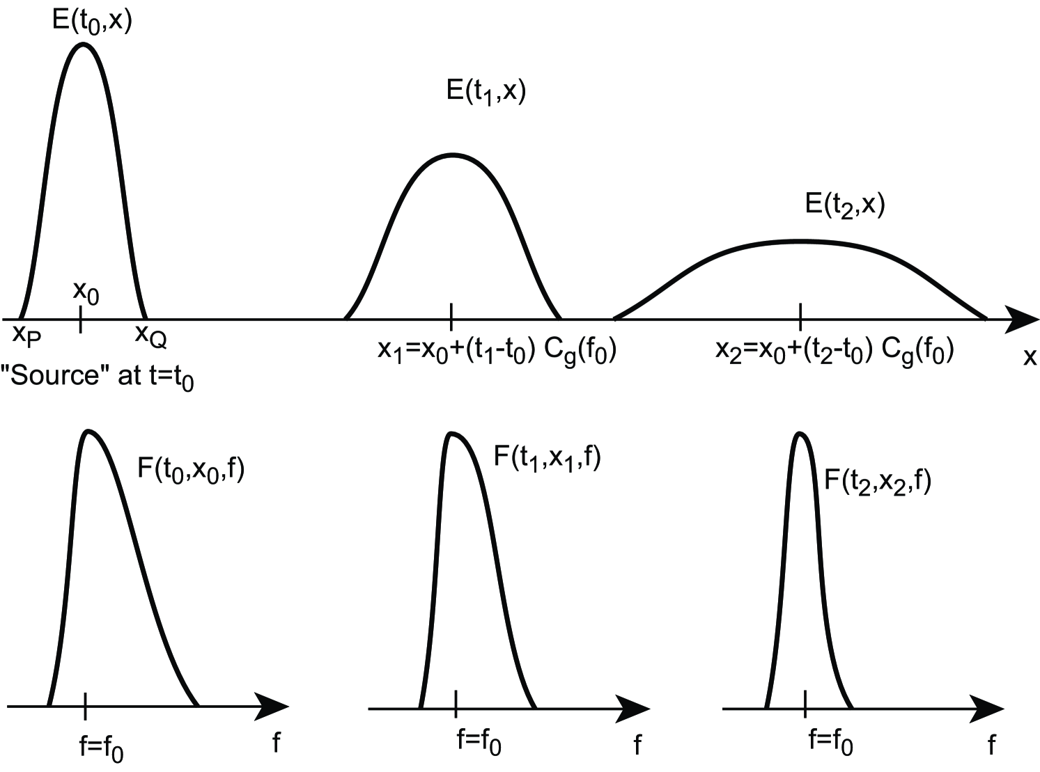
All these illustrations of forward-backward ray tracing indicate the potential to use a simple Geometrical Optics (GO) strategy. The next goal is then to determine the strength of the far-field radiated swell energy. This requires the definition of a swell source, and an estimation of the swell energy dissipation scale. For this we define the time as an initial condition after which there is no significant wave generation or non-linear evolution, for frequencies less than . Namely, at all the wave components with smaller frequencies have already been generated, so that the radiation of these waves is essentially fossil and fully governed by geometrical optics. The possible effects of diffraction and scattering are discussed by Munk et al. (1963), and, together with dissipation, will cause deviations from the G.O. model outlined below. We therefore make no restrictive hypothesis on what happens before , and thus the motion of the generating storm has no direct effect on our results, but it obviously modifies the spatial distribution of the energy at , which will be relevant.
In reality, swells evolve over the course of their propagation as the result of their interactions with the local winds, mutual wave-wave interactions, interactions with other wave systems, including the local wind sea. Swells are also expected to evolve according to interactions with other oceanic motions that affect the upper ocean, namely surface currents, internal waves (e.g. Kudryavtsev, 1994) and turbulence. Depth and island scattering effects must also carefully be taken into account (Snodgrass et al., 1966; WISE Group, 2007). Compared to these different mechanisms, frequency dispersion and angular spreading effects are certainly the first leading order phenomena to take into account for the major part of the decrease in the height of the swell systems. Indeed, as the long swell systems will be characterized by relatively small steepness parameters, nonlinear mutual wave-wave interactions do not appear to be important in scattering surface wave energy more than a few storm radius distances outside an active generating area Hasselmann (1963). Furthermore, the level of turbulence in the ocean does not appear to significantly affect the waves Fabrikant and Raevsky (1994); Ardhuin and Jenkins (2006), and the conversion of surface wave energy into internal gravity wave energy by wave-wave interactions does not seem to be a leading order sink term for the energy balance of surface gravity waves. Finally, for the very long trans-ocean fast propagating swell components, surface current bending effects, proportional to the ratio between vertical current vorticity and the group velocity, may also be considered as residual effects. Away from island obstructions, the ratio between the angular width along the great-circle observatory points at very large distances from the generating area, and the mean spread in the generating area is approximately proportional to with the spherical distance from the storm. center The change in spectral density defined by
| (5) |
follows the spatial expansion (close to the source) and contraction (as waves approach the antipodes for ) of the energy front. This transversal dispersion is associated to a narrowing of the directional spectrum , for , and a broadening for larger distances.
This approximation applies to large distances, and relatively small source regions. Closer to the source, the approximation does not hold. Swell amplitudes radiating from large extended sources will decrease more slowly than swell amplitudes emanating from compact sources.
Moreover, we can represent swell waves as a linear superposition of harmonic waves in narrow spectral band. Quite naturally, through the method of stationary phase, the group velocity is defined and the slowly-varying wave envelope is found to decay. This decay is inversely proportional to the square-root of the distance (figure 5). Accordingly, far away from the generating sources, and in the absence of dissipation, the swell energy
| (6) |
should decrease asymptotically like when following a wave group (see Appendix C for a detailed proof).
3.1 The Snodgrass et al. (1966) method
Using measurements with a limited or no directional resolution, Snodgrass et al. (1966) assumed that wave propagation was completely blocked by waters shallower than 60 fathoms (approximately 110 m), and that diffraction could be neglected. For example, in figure 6, the island would be represented by the 60 fathom depth contour. These authors then estimated a loss of swell energy from the deviation of the ratio of directionally-integrated spectra, e.g. , compared to what is expected from the lateral dispersion effect, taking into account islands. Currents, shallow water areas and diffraction effects around islands are neglected here. These effects are discussed by Snodgrass et al. (1966).
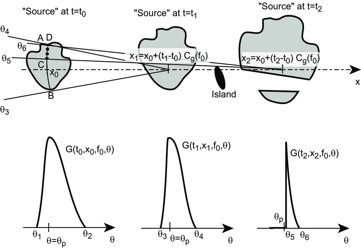
Rigorously, their method is inexact because the recording stations and measure wave groups that had neither exactly same propagation directions nor the same position when they were near . Yet, because the wave field in the neighborhood of is the superposition of many independent wave trains, one can assume that the spectral density is a smooth function of the direction. Then we may say that over the intervals to or to , does not change so much, i.e. in figure 6, . On the sphere the application of eqs. (1) and (5) yields
| (7) |
where the integral is performed over the line segment joining to . The error relative to the asymptote is the sum of two terms. One is proportional to the spatial gradient of , due to the change from the arc circle to the segment, and the other corresponds to the relative variation of with over the range to , which is small in the far field, provided that the directional spectrum is smooth enough.
Under these two smoothness assumptions, and for large , the ratios of spectral densities at and , as used by Snodgrass et al. (1966), can be compared to the conservative equations (7) and used to diagnose the dissipation of swell energy. This does not apply if is in the vicinity of the storm or its antipode, where the observed arrival direction span a large range.
In practice, this method can be very sensitive to the correct estimation of the island shadowing. For that reason, the measurement route chosen by Snodgrass et al. (1966) was far from ideal. Because they needed land to install most recording stations for the wave measurements, they used an almost north-south great circle that extends from the south of New-Zealand (Cape Palisader) to Alaska (Yakutat), a route peppered with islands in its southern part, and partially blocked by the Hawaiian chain in its northern part. Also, storms typically refuse to line up with any measurement array. Their pre-defined great circle, although designed to follow a typical Southern winter swell propagation path, always deviated by some extent form the actual track followed by the most energetic swells they recorded. For the Indian ocean storms, this difficulty was reduced by the relatively narrow range of angles that allows propagation from the Indian to the Pacific ocean.
3.2 A method using global swell heights
Now using an instrument with a global coverage, we can carefully avoid both problems by choosing propagation paths far away from the smallest island, and by exploiting only observations well aligned with the storms. However, due to the limited spectral resolution inherent to the SAR wave mode image size and processing, we cannot use the spectral distribution or of the energy, and can only use the energy integrated over a swell partition. We thus need for the equivalent of eq. (7) for .
For simplicity, and without loss of generality, we take the source storm centered at time on the pole defined by a colatitude , so that the distance from the storm center is . We consider the swell energy observed at a position defined by the spherical distance and we take the reference meridian to be in the direction of the observation point (figure 7).
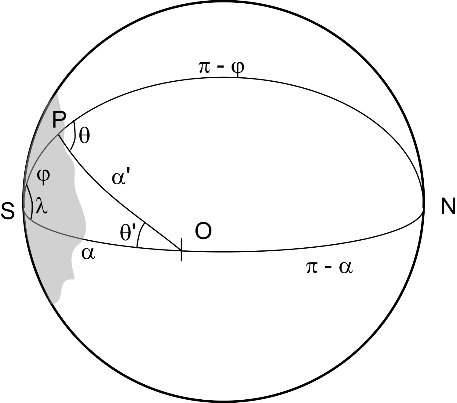
We will later assume that the source area is relatively small with a size , where is the maximum value taken by (figure 7). In all the following derivations, we have chosen a fixed frequency and we follow a wave group of that frequency. The time of observation is thus related to by , so that the variable will be omitted.
In appendix C, we prove and verify that, in the absence of dissipation the swell energy decreases like for large values of , and that typical storms should produce swells within 20% of this asymptote at distances larger than 4000 km from the storm center. A much larger observed deviation should thus reflect a gain or loss of energy by the propagating swells. The expected departures from the asymptotic evolution should be compared to those due to swell dissipation or generation. Even with perfect SAR observations, this is the intrinsic limit of the present method. A 20% error in energy conserving conditions may be misinterpreted as a dissipation or generation with an e-folding scale of the order of km, which gives a 20% energy change as waves propagate from 4000 to 8000 km away from the storm source.
3.3 Illustration
To illustrate the method described above, we analyse of one of the most powerful swell field recorded over the past 4 years by ENVISAT’s ASAR. The swell case illustrated in figure 4 is not well suited due to the islands in the south-north swell tracks and the poor sampling of ENVISAT for the tracks going north-east from the storm, we have thus chosen another source, found on February 12 2007 at 18:00 UTC, and located at 168 E and 38 N. This swell was generated by a storm moving Eastward with maximum Westerly winds of 26 m s-1 at the indicated date, and subsiding to less that 22 m s-1 and veering to South-Westerly 12 h later (according to ECMWF 0.5∘ resolution analyses). The storm motion in the direction of wave propagation certainly helped to amplify the local windsea, with a maximum significant wave height of 14.1 m at 00:00 UTC on February 13 (according to a numerical wave model configuration that is otherwise verified to produce root mean square errors less than 9% for m).
Using SAR-measured wave periods and directions at different times and locations, we follow great circle trajectories backwards at the theoretical group velocity. The location and date of the swell source is defined as the spatial and temporal center of the convergence area and time of the trajectories.
We chose a central peak period, here 15 s, and track the swells forward in space and time, starting from the source center at an angle , following ideal geodesic paths in search of SAR observations. Along each track, SAR data are selected if they are acquired within 3 hours and 100 km from the theoretical time and position. Great circle tracks are traced from the source in all directions, except for angular sectors with islands.
In order to obtain enough SAR data, we repeat this operation for regularly spaced values of with a step of . In our case, when varying from 74 to 90∘ (counted clockwise from North), this procedure produced 58 SAR measurements with one swell partition that had a peak wavelength and direction within 50 m and 20∘ of the expected theoretical value.
If no energy is lost by the wave field, decreases asymptotically as away from the source. Among the 58 swell observations, we further removed all the data within 4000 km of the source center, to make sure that the remaining data are in the far field of the storm, and data with a significant swell height less than 0.5 m, after bias correction based on the error model. This makes sure that the signal to noise ratio in the image is large enough so that the wave height estimation is accurate enough.
We then have 35 observations for which we assume that is only a function of , and we define the dissipation rate
| (8) |
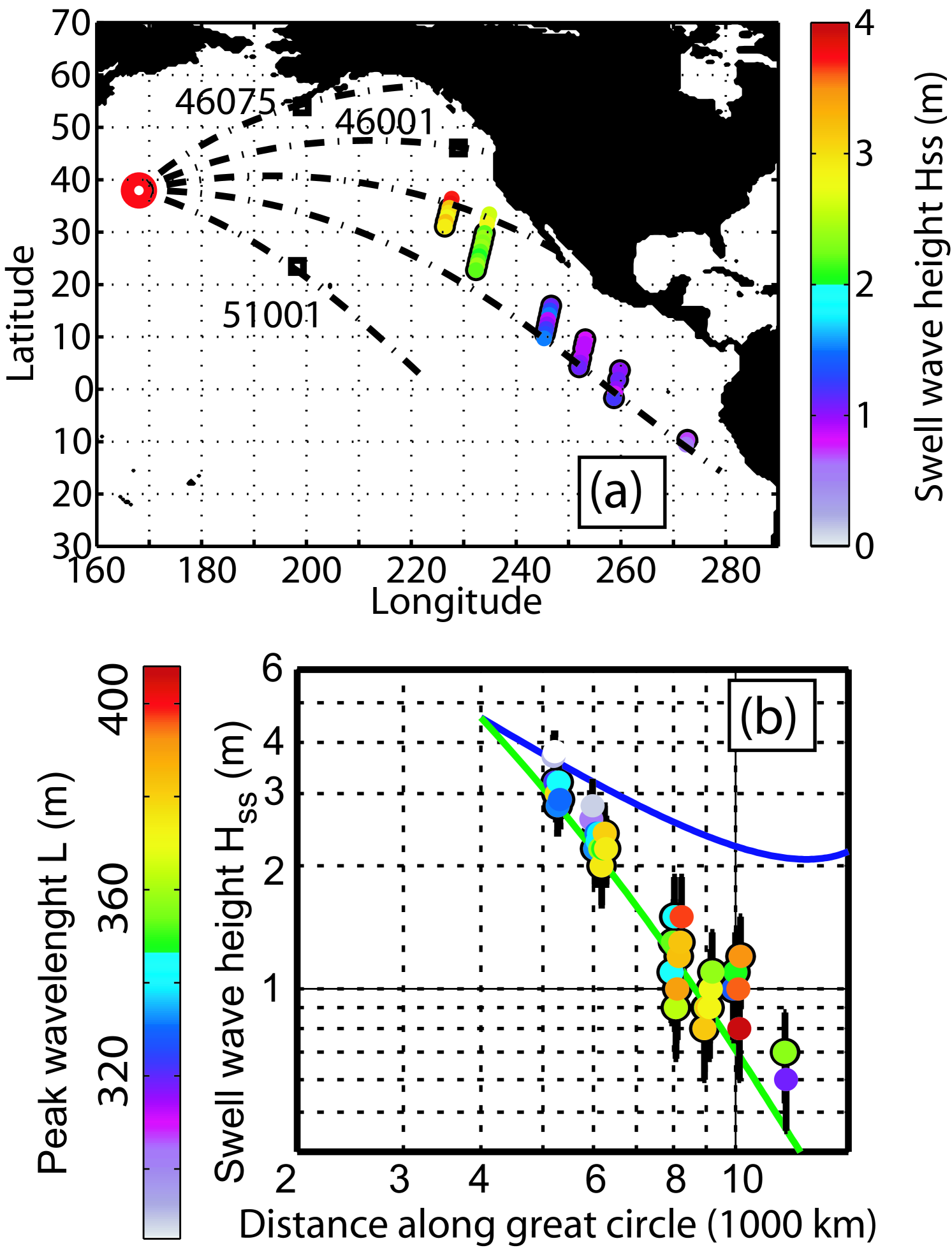
Positive values of correspond to losses of wave energy (figure 8). We then fit an analytical function to the data, defined by a constant and , i.e. the swell height at 4000 km from the source. Here the couple m and m-1 gives the least square difference between the decay with constant and the observed swell decays. Further, the uncertainty of that dissipation rate may be estimated from the known uncertainty of the SAR measurement of , given by eq. (3)-(4). A more simple error model, with larger errors based on the analysis by Johnsen et al. (2006), does not significantly alter this analysis. Using that error model and neglecting other sources of error in the present analysis, we perturbed the observed swell heights independently to produce a 400 ensemble of synthetic data sets. Taking the 16% and 84% levels in the estimation of , that would correspond to one standard deviation for a Gaussian distribution, we find that at the 68% confidence level. This is the first ever estimation of the uncertainty on an observed swell dissipation rate. These values of are more than twice larger than reported by Snodgrass et al. (1966) for smaller amplitude swells.
The formidable height of 4.4 m at a distance of 4000 km was observed by the SAR for all outgoing directions from at least to . This same swell was also recorded by buoys in the North-East of Hawaii (NDBC buoy 51001), also with a peak period of 15 s, and a height of 3.4 m on 16 February 2007 at 0:00 UTC. That buoy is located 3300 km away from the center and in a direction close to 112∘. Looking in the North-East quadrant of the storm, one also finds a trace of the swell at buoy 46005, off the Washington coast (4900 km in direction 59∘). There the swell was also observed with a 15 s period and a maximum height of 3.2 m on February 17 at 17:00 UTC, similar to the SAR observations for the same distance. For directions closer to Northbound, either the generation was weaker or the Alaskan islands sheltered the coastal buoys. For example, the same swell was also recorded by NDBC buoy number 46075, off Shumagin Island, Alaska, at a distance of 3000 km from the source, in the direction 42∘. At that buoy, the peak period was 15.0 s with a maximum swell height of 1.3 m on 15 February 2008 at 18:30 UTC.
Thus the power radiated by the storm is of the order of is 0.5 TW at 4000 km from the storm center, spread over a 50∘ angular sector. This power is about 16% of the estimated 3.2 TW annual mean flux that reaches the world’s coastlines (Rascle et al., 2008). However, the observed dissipation rate corresponds to an e-folding scale of 3300 km for the energy. Taking an average propagation distance of 8000 km, only 160 GW would make it to the shore. If the same dissipation rate prevailed closer to the source, then the power radiated at 1000 km form the storm center was 1.4 TW.
We thus expect that the far field dissipation of swells, in spite of the small steepness of these swells, plays a significant role in the air-sea energy balance. This effect probably explains the systematic positive bias for predicted wave heights in wave models that neither account for swell dissipation nor assimilate wave measurements (see e.g. Rascle et al., 2008).
4 Conclusions
Taking advantages of the satellite observations of unprecedented coverage and quality, investigations can repeat and complement the pioneering analysis of swell evolution performed in the 1960s. Severe storms can generate relatively broad spectra of large surface waves. But rapidly, the redistribution of energy, through linear dispersion and nonlinear interaction mechanisms, becomes very effective. The initial wind waves become swells outrunning the wind, leading to the apparition long-crested systems. The propagation properties of these surface gravity waves have been found to closely follow principles of geometrical optics. The consistent patterns of swell fronts dispersing over thousands of kilometers was shown to be useful to provide time series at ”virtual wave observing stations”, filling gaps in space and time in between the orbit cycles of observation. When compared to buoy measurements, the present results give an explicit dynamical validation of the SAR-derived spectral parameters. As the speed of waves in deep water is proportional to their period or wavelength, information carried by the SAR-derived period and direction distributions, observed at a fairly large distance from the generating area, pertains to the wind conditions existent up to 15 days before.
We also discussed how the swell energy should, in the absence of dissipation, decay in the far field of the storm like where is the spherical distance between the storm center and observation point. Exploiting that property allowed us to estimate a dissipation rate of swell energy with unprecedented accuracy, establishing that swell dissipation can be a significant term in the global wave energy budget.
The proposed methodolgy performed here requires data far enough from the source, typically more than 4000 km, in order to approach this simple asymptotic behavior. At the same time, the swell amplitude should be large enough to be accurately measured by the SAR. Some knowledge of the spectral shape and its spatial distribution inside the storm may be useful to provide better estimates of for low dissipation cases, or closer to the storm centers. These further analyses will likely benefit from the joint use of data from altimeters, SARs, and other sources of spectral wave information.
A more systematic analysis and interpretation of this dissipation will be reported elsewhere (Ardhuin et al., 2009a), with applications to wave forecasting models (Ardhuin et al., 2008, 2009b). The parameterization of the dissipation rate could also be used to produce a data-based forecasting system, extending our virtual buoy technique to the estimation of swell heights, with a forward propagation of observations.
Going in the opposite direction, toward the storm source, it is possible that the analysis of swell fields could provide a ”new” way of looking into the poorly observed structure of severe storms. Because the usual remote sensing techniques for estimating wind fields either do not work for very high winds or are not well validated (e.g. Quilfen et al., 2006, 2007), the use of far-field swell information may provide an interesting complement to the local wind speeds and wave heights. The is inverse problem has already been formulated by Munk et al. (1963) who already proposed an elegant heterodyning technique to push the spatial resolution for the estimation of storm location from swell data, while Heimbach and Hasselmann (2000) have proposed to use wave models to correct wind field errors. The quality of the SAR-derived swell parameters that are coming out of today’s ENVISAT and tomorrow’s Sentinel-1, together with a good understanding of the swell energy budget, including its dissipation revealed here, may finally enable this vision.
Appendix A Viscous theory for air-sea interaction
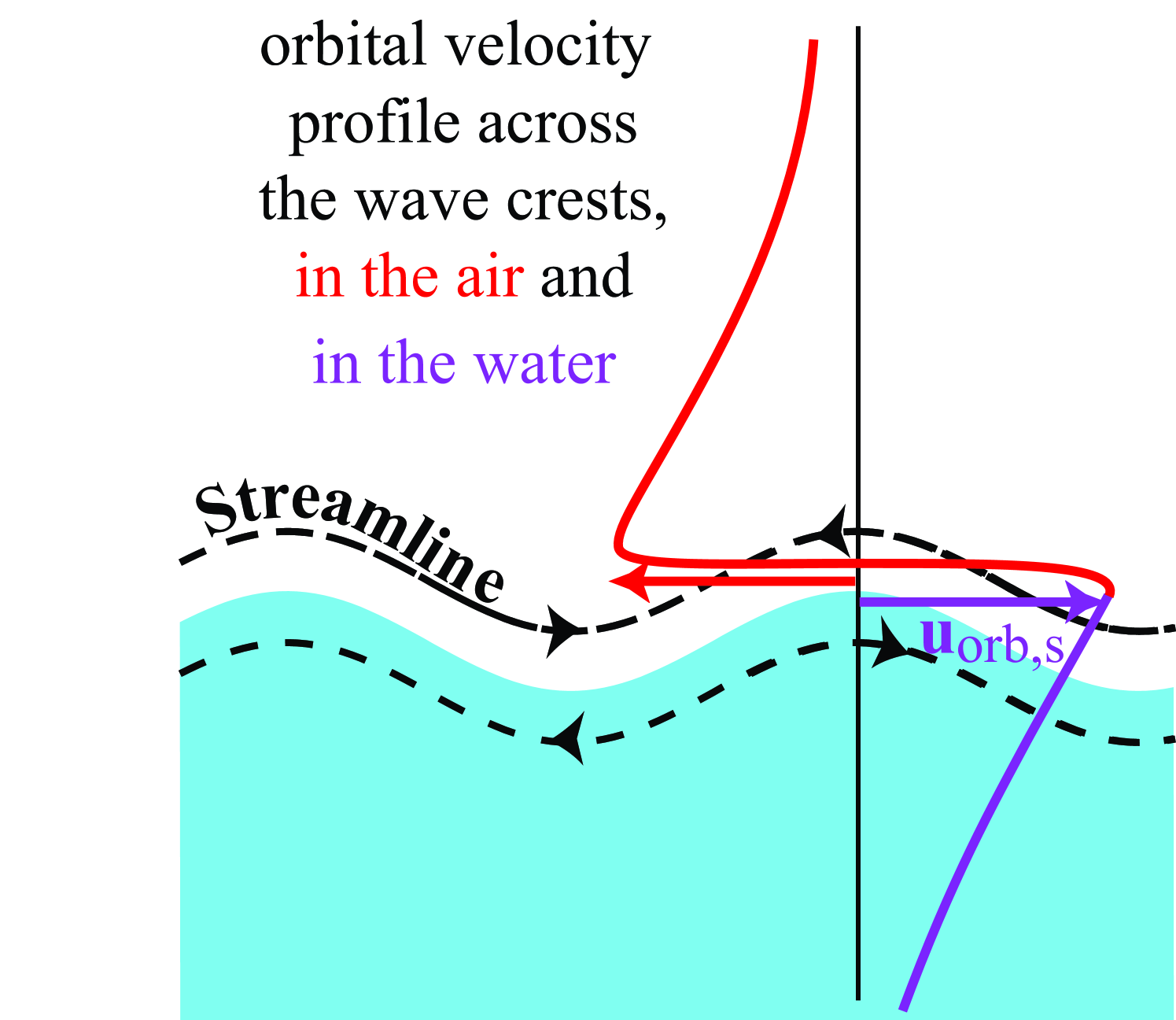
For the sake of simplicity we will consider here the case of monochromatic waves propagating in the direction only, and we will neglect the curvature of the surface. For the small steepness swells considered here that latter approximation is well founded and a more complete analysis is given by Kudryavtsev et Makin (2004). For deep water waves, the free stream velocity above the waves, just outside of the boundary layer is , where is the swell amplitude and is the radian frequency. The sub-surface velocity is (figure 9). Due to the oscillations that propagate at the phase velocity , the horizontal advection of any quantity by the flow velocity , given by , can be neglected compared to its rate of change in time since the former is a factor smaller than the latter, which is typically less that 0.1 for the swells considered here. Defining , where the brackets denote an average over flow realizations for a given wave phase. The horizontal momentum equation is thus approximated by,
| (9) |
where represents the divergence of the vertical viscous and turbulent fluxes of horizontal momentum,
| (10) |
Because the boundary layer thickness is small compared to the wavelength, the pressure gradient in the boundary layer is given by the pressure gradient above the boundary layer, in balance with the horizontal acceleration. This is another way to write Bernoulli’s equation (e.g. Mei 1989),
| (11) |
This yields
| (12) |
with the boundary condition for , goes to . The equation for the horizontal momentum is thus exactly identical to the one for the oscillatory boundary layer over a fixed bottom with wave of the same period but with an amplitude twice as large. In the viscous case, and one recovers, after some straightforward algebra, the known viscous result, i.e., for ,
| (13) |
where , with the surface elevation .
The dissipation rate of energy is given by the mean work of the viscous stresses,
| (14) |
Equation (13) gives,
| (15) |
This gives the low frequency asymptote to the viscous decay coefficient (Dore, 1978),
| (16) |
This result was previously obtained using a Lagrangian approach without all the above simplifying assumptions (Weber and Førland, 1990, their equation 7.1 in which our correspond to their ). The full viscous result is obtained by also considering the water viscosity , which gives the correction for the motion in the air, and the classical dissipation term with a decay , which dominates for the short gravity waves.
The total disspation rate is simply . For a clean surface with m2 s-1, m2 s-1, and , the two terms are equal for waves with a period s and a wavelength of 2.6 m. The air viscosity dominates for all waves longer than this, which is typically the range covered by spectral wave models for sea state forecasting.
For a comparison with fixed bottom boundary layers, the Reynolds number based on the orbital motion should be redefined with a doubled velocity and a doubled displacement, i.e. Re. For monochromatic waves and . For random waves, investigations of the ocean bottom boundary layer suggest that the boundary layer properties are roughly equivalent to that of a monochromatic boundary layer defined by significant properties (Traykovski et al. 1999).
Although the wind was neglected here, it should influence the shear stresses when its vertical shear is of the order of the wave-induced shear. Taking a boundary layer thickness and wind friction velocity , and assuming a logarithmic wind profile, this should occur when exceeds , where is von Kármán’s constant. This corresponds to, roughly, . For swells with T s and m (i.e. m s-1), and winds less than 7 m s-1 (i.e. m s-1), the wind effect on may be small and the previous analysis is likely valid. In general, however, the nonlinear interaction of the wave motion and wind should be considered, which requires an extension of existing theories for the distortion of the airflow to finite swell amplitudes.
Finally, the above result for the air viscosity is easily generated to any water depth by dividing the free stream velocity by , so that the dissipation rate is a factor larger in intermediate water depth.
Appendix B Quantitative validation of
A classical analysis of SAR estimation errors is provided by a direct comparison of swell parameters, estimated from level 2 products, with buoy measurements at nearly the same place and time (Holt et al., 1998; Johnsen and Collard, 2004).
Previous validations were presented for the total wave height (Collard et al., 2005) or a truncated wave height defined by chopping the spectrum at a fixed frequency cut-off of Hz. For that parameter, Johnsen and Collard (2004) found a root mean square (RMS) difference of 0.5 m, when comparing SAR against buoy data, including a bias of 0.2 m. In the present study, we use values obtained from both SAR and buoy spectra.
For each wave spectrum observed in the world ocean, swell partitions are extracted providing estimations of , , and . In practice, the L2 spectra are first smoothed over 3 direction bins (30∘ sectors) and 3 wavenumber bins, in order to remove multiple peaks that actually correspond to the same swell system. The peaks are then detected and the energy associated to each peak is obtained by the usual inverted water-catchment procedure (Gerling, 1992). The swell peak period is defined as the energy-weighted average around % of the frequency with the maximum energy. Likewise the peak direction is defined as the energy-weighter direction within 30∘ of the peak direction.
A preliminary validation of was performed by Collard et al. (2006), using L2 processing applied to 4 by 4 km tiles from narrow swath images exactly located at buoy positions. That study found a 0.37 m r.m.s. error. This smaller error was obtained in spite of a 4 times smaller image area that should on the contrary produce larger errors due to statistical uncertainties. This suggests that a significant part of the ”errors” in SAR validation studies are due to the distance between SAR and buoy observations.
The swell height validation has been repeated here, using all buoy data from 2004 to 2008, located within 200 km and 1 hour of the SAR observation. These co-located data are made publically available as part of the XCOL project on the CERSAT ftp server, managed by Ifremer. Because we wished to avoid differences due to coastal sheltering and shallow water effects, we restricted our choice of buoys to distances from the coast and the 100 m depth contour larger than 100 km. As a result, most selected buoys are not directional, and we use partitions in frequency only. For the present validation, differently from other section of this paper, we thus define a swell partition as the region between two minima of the frequency spectrum. The corresponding energy gives the swell height . The buoy swell height is then defined from the energy contained within the frequency band of the SAR partition. The peak period is then estimated as the period where the buoy spectrum is maximum. The database includes 15628 swell partitions observed by the SAR, with matched buoy swell partitions.
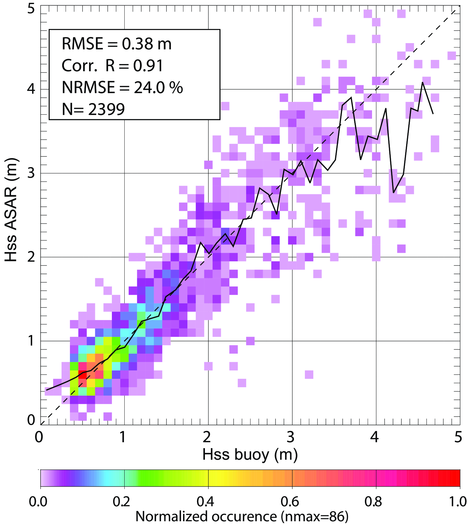
Many of these observations correspond to relatively short swells, for which the waves are poorly imaged. We have thus defined a subset of the database by imposing the following conditions. First the image normalized variance, linked to the contrast intensity and homogeneity, should be in the range 1.05 to 1.5, which limits the dataset to 6651 observations. This removes SAR data with non-wave features (slicks, ships …) that would otherwise contaminate the wave spectra. Second, both the SAR and buoy peak periods are restricted to the 12 to 18 s range, which reduces the dataset to 4136 observations, and removes most of the problems related to the azimuthal cut-off. Third and last, the SAR-derived wind speed is limited to range from 3 to 9 m s-1 in order to remove low winds with poorly contrasted SAR images and high winds which may still cause some important azimuthal cut-off and contamination of swell spectra by wind sea spectra. This gives subset A, with 2399 observations. The resulting heights are compared to buoy measurements in figure 10.
When the maximum wind is reduced to 8 m s-1, giving subset B, the differences between SAR and buoy data is reduced, with further reductions when the maximum distance between SAR and buoy data is reduced from 200 to 100 km to give subset C (table 1).
| \tableline | ||
|---|---|---|
| subset A, bias | 0.00 m | 0.27 s |
| subset A, RMSE | 0.38 m | 1.14 |
| subset A, S.I. | 24.0% | 7.9% |
| subset A, NRMSE | 24.0% | 8.2% |
| subset A, | 0.91 | 0.61 |
| \tableline | ||
| subset B, bias | 0.00 m | 0.24 s |
| subset B, RMSE | 0.35 m | 1.11 s |
| subset B, S.I. | 23.5% | 7.8% |
| subset B, NRMSE | 23.5% | 8.0% |
| subset B, | 0.92 | 0.62 |
| \tableline | ||
| subset C, bias | 0.02 m | 0.32 s |
| subset C, RMSE | 0.29 m | 1.07 s |
| subset C, S.I. | 22.4% | 7.3% |
| subset C, NRMSE | 22.5% | 7.7% |
| subset C, | 0.92 | 0.64 |
| \tableline |
Appendix C Derivation and verification of the asymptotic swell energy without dissipation
C.1 Derivation
The swell energy is an integral of the local spectrum over both frequencies and arrival directions ,
| (17) |
Using eq. (1) this local integral, can also be written as an integral over the entire source area . The spherical distance between any point in the source region and the observation point is . The observed frequency that is due to this source point is
| (18) |
We may replace by in eq. (17),
| (19) |
For a circular uniform storm of radius with isotropic spectra, as used in figure 11, is given by the integral over weighted by the directional width of the spectrum . That width is given by the spherical trigonometry relationship
| (20) |
with .
For general spectral distribution, we may transform the integration variables which are the colatitude and longitude coordinates on the sphere with a pole at the observation point, to coordinates with a pole in the center of the swell field at . The transformation Jacobian is simply given by the equality of the elementary area on the unit radius sphere . We thus have
where is the direction of the great circle at the generation point that goes through that point and the observation point. is thus a function of , , and . is maximum value of , i.e. the radius of the source region divided by the Earth radius.
For continuous spectra, the second integral on the right hand side of eq. (17) goes to zero as goes to infinity (which, on the sphere is limited by ) since the part of the source spectra that contribute to the observations shrink to a smaller and smaller neighborhood around and . The observed frequencies are limited by
| (23) |
This is enough to guarantee that this second integral also contributes a deviation from the asymptote, limited by
| (24) |
where the maximum is taken over all the contributing components.
Similarly, the outgoing directions received at the observation point are also limited to a narrow window as increases, giving another deviation term . Using the sine formula in the triangle , . Thus, in the far field of the storm and its antipode, is close to . Thus , which is less than , and therefore is less than . If one does not get too close to the storm or its antipode (say, ) then we can give an upper bound of as a function of and obtain
| (25) |
The deviation from the asymptote due to is thus of the order of and may increase close to the antipode, if waves from a wide range of directions can reach that point. In practice this does not happen since continents and island chains block most of the arrival directions at the antipode, leaving only a small window of possible arrival directions (e.g. Munk et al., 1963). Directional wave spectra in active generation areas are generally relatively broad with typically less than 2 for directions within 30∘ of the main wave direction. On the contrary, typical storm spectra can give as large as 10 for frequencies within 30% of the peak frequency. We thus expect the deviation to dominate over .
C.2 Verification
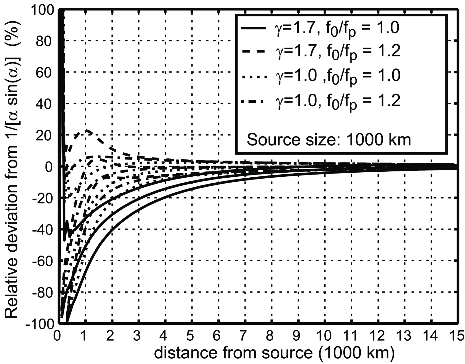
For a useful comparison with observations, the asymptotic swell height evolution should be approached on a scale smaller than the ocean basin scale. This is easily tested for storms with spatially uniform spectra over a radius , by evaluating the integral in eq. (19). We chose a center frequency and consider the swell energy at a distance and a time such that . is thus an error relative to the theoretical position of the wave group of frequency . The relative difference of and its asymptotic evolution depends only on the spectral shape in the storm, the relative frequency where is the peak frequency, the distance , the storm size , and the position error . Results are shown in figure 11 for isotropic directional spectra, in which case . Although an isotropic spectrum is not realistic at all, it allows for simple calculations. As discussed below, the effect of directional spreading is expected to be less important than the shape of the frequency spectrum.
As indicated by eq. (24), the contribution of both the spectral shape and comes through the maximum relative variation of in the frequency interval that contribute to . Here we take the spectra in the storm to have a JONSWAP shape (Hasselmann et al., 1973), that we adjust by varying the peak enhancement factor . A relatively broad Pierson and Moskowitz (1964) spectrum is obtained with . If we chose , this spectrum will give smaller deviations of from the asymptote (solid lines in figure 11), than narrower spectra with larger values of . Young (2005) showed that wave spectra in Hurricanes generally fall in between these two categories, with a typical value . Larger deviations from the asymptote are obtained for , since the forward face of the spectrum is very steep, while smaller errors are obtained for due to the more gentle decrease of towards the high frequencies.
Similarly, large deviations are produced if the observations are made in a direction far from the peak generation direction in cases when the directional spectrum is narrow. For observation directions 30∘ from the peak direction, and spectra with a directional distribution, the deviations are still dominated by the dispersive term , as expected.
The other important factor is the distance relative to the storm size . A faster convergence is obtained for smaller storms. If observations do not correspond exactly to a theoretical propagation at a group speed but are within a distance of the theoretical position, the values of will also be affected in a way that depends on the spectral shape. In the absence of energy gains or losses, and for realistic storm sizes and spectral shapes, the deviation of observations from the asymptote should be less than 20% for km when km is enforced.
Acknowledgements.
SAR data was provided by the European Space Agency (ESA) and buoy data was kindly provided by the U.S. National Data Buoy Center, and Marine Environmental Data Service of Canada. ESA funded the XCOL co-located database and the initial work on the virtual buoy concept. The swell decay analysis was funded by the French Navy as part of the EPEL program. This work is a contribution to the ANR-funded project HEXECO and DGA-funded project ECORS.References
- Aouf et al. (2006) Aouf, L., J.-M. Lefèvre, D. Hauser, and B. Chapron (2006), On the combined assimilation of RA-2 altimeter and ASAR wave data for the improvement of wave forcasting, in Proceedings of 15 Years of Radar Altimetry Symposium, Venice, March 13-18.
- Ardhuin and Jenkins (2006) Ardhuin, F., and A. D. Jenkins (2006), On the interaction of surface waves and upper ocean turbulence, J. Phys. Oceanogr., 36(3), 551–557.
- Ardhuin et al. (2008) Ardhuin, F., F. Collard, B. Chapron, P. Queffeulou, J.-F. Filipot, and M. Hamon (2008), Spectral wave dissipation based on observations: a global validation, in Proceedings of Chinese-German Joint Symposium on Hydraulics and Ocean Engineering, Darmstadt, Germany.
- Ardhuin et al. (2009a) Ardhuin, F., B. Chapron, and F. Collard (2009a), Observation of swell dissipation across oceans, Geophys. Res. Lett., in press.
- Ardhuin et al. (2009b) Ardhuin, F., L. Marié, N. Rascle, P. Forget, and A. Roland (2009b), Observation and estimation of Lagrangian, Stokes and Eulerian currents induced by wind and waves at the sea surface, J. Phys. Oceanogr., submitted, available at http://hal.archives-ouvertes.fr/hal-00331675/.
- Breivik et al. (1998) Breivik, L. A., M. Reistad, H. Schyberg, J. Sunde, H. E. Krogstad, and H. Johnsen (1998), Assimilation of ERS SAR wave spectra in an operational wave model, J. Geophys. Res., 103, 7887–7900.
- Chapron et al. (2001) Chapron, B., H. Johnsen, and R. Garello (2001), Wave and wind retrieval from SAR images of the ocean, Ann. Telecommun., 56, 682–699.
- Collard et al. (2005) Collard, F., F. Ardhuin, and B. Chapron (2005), Extraction of coastal ocean wave fields from SAR images, IEEE J. Oceanic Eng., 30(3), 526–533.
- Collard et al. (2006) Collard, F., B. Chapron, F. Ardhuin, H. Johnsen, and G. Engen (2006), Coastal ocean wave retrieval from ASAR complex images, in Proceedings of OceanSAR, Earth Observation Marine Surveillance Coordination Comittee, Saint John’s, Canada.
- Darbyshire (1958) Darbyshire, J. (1958), The generation of waves by wind, Phil. Trans. Roy. Soc. London A, 215(1122), 299–428.
- Dore (1978) Dore, B. D. (1978), Some effects of the air-water interface on gravity waves, Geophys. Astrophys. Fluid. Dyn., 10, 215–230.
- Engen and Johnsen (1995) Engen, G., and H. Johnsen (1995), Sar-ocean wave inversion using image cross spectra, IEEE Trans. on Geosci. and Remote Sensing, 33, 4.
- Fabrikant and Raevsky (1994) Fabrikant, A. L., and M. A. Raevsky (1994), The influence of drift flow turbulence on surface gravity wave propagation, J. Fluid Mech., 262, 141–156.
- Gerling (1992) Gerling, T. W. (1992), Partitioning sequences and arrays of directional ocean wave spectra into component wave systems, J. Atmos. Ocean Technol., 9, 444–458.
- Gjevik et al. (1988) Gjevik, B., H. E. Korgstad, A. Lygre, and O. Rygg (1988), long period swell wave events on the Norwegian shelf, J. Phys. Oceanogr., 18, 724–737.
- Grachev and Fairall (2001) Grachev, A. A., and C. W. Fairall (2001), Upward momentum transfer in the marine boundary layer, J. Phys. Oceanogr., 31, 1698–1711.
- Hanson and Phillips (2001) Hanson, J. L., and O. M. Phillips (2001), Automated analysis of ocean surface directional wave spectra, J. Atmos. Ocean Technol., 18, 277–293.
- Hasselmann (1963) Hasselmann, K. (1963), Part 3. evaluation on the energy flux and swell-sea interaction for a Neuman spectrum, J. Fluid Mech., 15, 467–483.
- Hasselmann et al. (1973) Hasselmann, K., et al. (1973), Measurements of wind-wave growth and swell decay during the Joint North Sea Wave Project, Deut. Hydrogr. Z., 8(12), 1–95, suppl. A.
- Hasselmann et al. (1996) Hasselmann, S., C. Brüning, and K. Hasselmann (1996), An improved algorithm for the retrieval of ocean wave spectra from synthetic aperture radar image spectra, J. Geophys. Res., 101, 16,615–16,629.
- Hasselmann et al. (1997) Hasselmann, S., P. Lionello, and K. Hasselmann (1997), An optimal interpolation scheme for the assimilation of spectral wave data, J. Geophys. Res., 102, 15,823–15,836.
- Heimbach and Hasselmann (2000) Heimbach, P., and K. Hasselmann (2000), Development and application of satellite retrievals of ocean wave spectra, in Satellites, oceanography and society, edited by D. Halpern, pp. 5–33, Elsevier, Amsterdam.
- Holt et al. (1998) Holt, B., A. K. Liu, D. W. Wang, A. Gnanadesikan, and H. S. Chen (1998), Tracking storm-generated waves in the northeast pacific ocean with ERS-1 synthetic aperture radar imagery and buoys, J. Geophys. Res., 103(C4), 7917–7929.
- Johnsen and Collard (2004) Johnsen, H., and F. Collard (2004), ASAR wave mode processing - validation of reprocessing upgrade. technical report for ESA-ESRIN under contract 17376/03/I-OL, Tech. Rep. 168, NORUT.
- Johnsen et al. (2006) Johnsen, H., G. Engen, F. Collard, V. Kerbaol, and B. Chapron (2006), Envisat ASAR wave mode products - quality assessment and algorithm upgrade, in Proceedings of SEASAR 2006, SP-613, ESA, ESA - ESRIN, Frascati, Italy.
- Kedar et al. (2008) Kedar, S., M. Longuet-Higgins, F. W. N. Graham, R. Clayton, and C. Jones (2008), The origin of deep ocean microseisms in the north Atlantic ocean, Proc. Roy. Soc. Lond. A, pp. 1–35, 10.1098/rspa.2007.0277.
- Kerbaol et al. (1998) Kerbaol, V., B. Chapron, and P. Vachon (1998), Analysis of ERS-1/2 synthetic aperture radar wave mode imagettes, J. Geophys. Res., 103(C4), 7833–7846.
- Krogstad (1992) Krogstad, H. E. (1992), A simple derivation of Hasselmann’s nonlinear ocean-synthetic aperture radar transform, J. Geophys. Res., 97(C2), 2421–2425.
- Kudryavtsev (1994) Kudryavtsev, V. N. (1994), The coupling of wind and internal waves, J. Fluid Mech., 278, 33–62.
- Kudryavtsev and Makin (2004) Kudryavtsev, V. N., and V. K. Makin (2004), Impact of swell on the marine atmospheric boundary layer, J. Phys. Oceanogr., 34, 934–949.
- Mei (1989) Mei, C. C. (1989), Applied dynamics of ocean surface waves, second ed., World Scientific, Singapore, 740 p.
- Munk and Traylor (1947) Munk, W. H., and M. A. Traylor (1947), Refraction of ocean waves: a process linking underwater topography to beach erosion, Journal of Geology, LV(1), 1–26.
- Munk et al. (1963) Munk, W. H., G. R. Miller, F. E. Snodgrass, and N. F. Barber (1963), Directional recording of swell from distant storms, Phil. Trans. Roy. Soc. London A, 255, 505–584.
- Pierson and Moskowitz (1964) Pierson, W. J., Jr, and L. Moskowitz (1964), A proposed spectral form for fully developed wind seas based on the similarity theory of S. A. Kitaigorodskii, J. Geophys. Res., 69(24), 5,181–5,190.
- Quilfen et al. (2006) Quilfen, Y., J. Tournadre, and B. Chapron (2006), Altimeter dual-frequency observations of surface winds, waves, and rain rate in tropical cyclone isabel, J. Geophys. Res., 87(111), C01,004, 10.1029/2005JC003068.
- Quilfen et al. (2007) Quilfen, Y., C. Prigent, B. Chapron, A. A. Mouche, and N. Houti (2007), The potential of quikscat and windsat observations for the estimation of sea surface wind vector under severe weather conditions, J. Geophys. Res., 112, C09,023, 10.1029/2007JC004163.
- Rascle et al. (2008) Rascle, N., F. Ardhuin, P. Queffeulou, and D. Croizé-Fillon (2008), A global wave parameter database for geophysical applications. part 1: wave-current-turbulence interaction parameters for the open ocean based on traditional parameterizations, Ocean Modelling, 25, 154–171, doi:10.1016/j.ocemod.2008.07.006.
- Schulz-Stellenfleth et al. (2005) Schulz-Stellenfleth, J., S. Lehner, and D. Hoja (2005), A parametric scheme for the retrieval of two-dimensional ocean wave spectra from synthetic aperture radar look cross spectra, J. Geophys. Res., 110, C05,004, 10.1029/2004JC002822.
- Schulz-Stellenfleth et al. (2007) Schulz-Stellenfleth, J., T. König, and S. Lehner (2007), An empirical approach for the retrieval of integral ocean wave parameters from synthetic aperture radar data, J. Geophys. Res., 21, C03,019, 10.1029/2006JC003970.
- Snodgrass et al. (1966) Snodgrass, F. E., G. W. Groves, K. Hasselmann, G. R. Miller, W. H. Munk, and W. H. Powers (1966), Propagation of ocean swell across the Pacific, Phil. Trans. Roy. Soc. London, A249, 431–497.
- Tolman (2002) Tolman, H. L. (2002), Alleviating the garden sprinkler effect in wind wave models, Ocean Modelling, 4, 269–289.
- Traykovski et al. (1999) Traykovski, P., A. E. Hay, J. D. Irish, and J. F. Lynch (1999), Geometry, migration, and evolution of wave orbital ripples at LEO-15, J. Geophys. Res., 104(C1), 1,505–1,524.
- Weber and Førland (1990) Weber, J. E., and E. Førland (1990), Effect of the air on the drift velocity of water waves, J. Fluid Mech., 218, 619–640.
- WISE Group (2007) WISE Group (2007), Wave modelling - the state of the art, Progress in Oceanography, 75, 603–674, 10.1016/j.pocean.2007.05.005.
- Young (2005) Young, I. R. (2005), Directional spectra of hurricane wind waves, J. Geophys. Res., 111, C08,020, 10.1029/2006JC003540.