S2MVTC: a Simple yet Efficient Scalable Multi-View Tensor Clustering
Abstract
Anchor-based large-scale multi-view clustering has attracted considerable attention for its effectiveness in handling massive datasets. However, current methods mainly seek the consensus embedding feature for clustering by exploring global correlations between anchor graphs or projection matrices. In this paper, we propose a simple yet efficient scalable multi-view tensor clustering (S2MVTC) approach, where our focus is on learning correlations of embedding features within and across views. Specifically, we first construct the embedding feature tensor by stacking the embedding features of different views into a tensor and rotating it. Additionally, we build a novel tensor low-frequency approximation (TLFA) operator, which incorporates graph similarity into embedding feature learning, efficiently achieving smooth representation of embedding features within different views. Furthermore, consensus constraints are applied to embedding features to ensure inter-view semantic consistency. Experimental results on six large-scale multi-view datasets demonstrate that S2MVTC significantly outperforms state-of-the-art algorithms in terms of clustering performance and CPU execution time, especially when handling massive data. The code of S2MVTC is publicly available at https://github.com/longzhen520/S2MVTC.
1 Introduction
The progress in information collection technology now permits us to gather multi-view data from the same object, presenting observations with depth and comprehensiveness. For instance, brain activity can be measured using functional Magnetic Resonance Imaging (fMRI) and Electroencephalography (EEG) [11, 26]. Benefiting from the consensual and complementary information, multi-view data have attracted a series of multi-view learning tasks [32, 1]. Among them, multi-view clustering, which groups data into several clusters by integrating information from different views, has been extensively applied in fields including image processing, computer vision, and neuroscience [29, 36, 3, 43].
Current multi-view clustering (MVC) methods, mainly based on self-representation learning or graph learning, aim to find the consensus embedding feature and have attained considerable advancements [4, 31, 22, 24]. However, for views and samples, these methods require updating membership graphs () to construct the affinity matrix, which will be then fed into spectral clustering algorithm [34]. Both storage and computational demands for these methods scale at a complexity of , where and represent the numbers of views and samples, respectively. These methods could be infeasible for large-scale datasets, particularly when is massive, and such scalability is important in real-world applications.
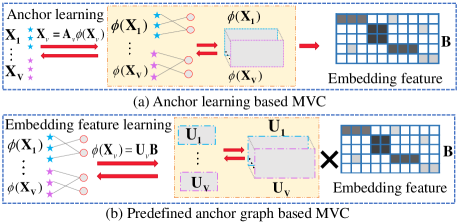
To address it, many anchor-based scalable MVC methods have been proposed for large-scale data [42, 20, 30, 37], where anchor graphs of size are constructed from anchors and samples () to approximately represent memberships between multi-view data. According to the differences in inter-view processing levels, these methods can be further subdivided into two categories. The first one relies on anchor learning, emphasizing the exploration of anchor graph consistency across views, as shown in Fig. 1 (a). Subsequently, the fused anchor graph is employed to construct the embedding feature, which will be fed into a -means algorithm for clustering [39, 42, 12, 24]. The second one relies on provided anchor graphs and learns the embedding feature using the projection matrices, as shown in Fig. 1 (b). It explores the consistency among projection matrices to acquire the compact embedding feature, which is then utilized for learning clustering structures [44, 35, 45].
The above-mentioned anchor-based methods either explore the global correlations between anchor graphs or projection matrices. However, their ultimate goal is to learn the consensus embedding feature, which directly impacts the clustering performance. Therefore, two questions naturally arise: Why not directly explore the correlations between embedding features from different views? Would this approach be more effective?
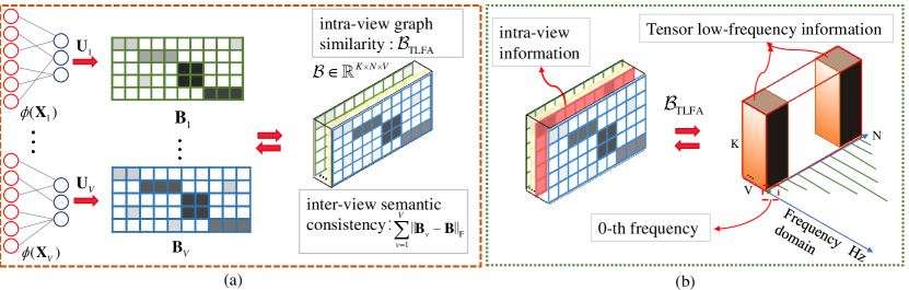
In this paper, we try to answer these questions and focus on learning inter-and intra-view consistency among embedding features. We propose a simple yet efficient scalable multi-view tensor clustering (S2MVTC) approach tailored for large-scale data. As depicted in Fig. 2, we initially map the anchor graph onto the projection matrix to obtain the embedding feature for each view. To ensure the consensus among intra-view embedding features effectively, we introduce a novel approach by employing a tensor low-frequency approximation (TLFA) on the embedding feature tensor, denoted as , where the tensor is formed by concatenating the embedding features from each view and subsequently rotating it. Benefiting from the fast Fourier transform (FFT) in the third mode of tensor singular value decomposition (t-SVD) [15], the newly defined TLFA can achieves the smooth representation of samples within different views [8].
Furthermore, to ensure inter-view semantic consistency, a consensus constraint is imposed on the embedding features. By incorporating these two parts into a unified framework, S2MVTC can efficiently leverage inter/intra-view information for large-scale MVC tasks. Ultimately, the clustering structure learning is applied to the well-learned embedding consensus feature to obtain the clustering results.
The main contributions are summarized as:
-
•
Different from existing anchor-based methods that explore global correlations between anchor graphs or projection matrices, S2MVTC directly learns both inter and intra-view embedding feature correlations.
-
•
Benefiting from the newly defined TLFA operator, S2MVTC achieves the smooth representation within different views.
-
•
Experimental results on six large multi-view datasets demonstrate that S2MVTC significantly improves the clustering performance compared to state-of-the-art algorithms, especially as the data size increases, making the advantages of S2MVTC more evident.
2 Notations and Problem Formulation
2.1 Notations
For clarity, we present notations frequently used in Tab. 1.
| Symbol | Definition |
|---|---|
| , , , and | A scalar, a vector, a matrix, and a tensor |
| Indices range from 1 to their capital version | |
| Fields of real numbers and complex numbers | |
| the complex conjugate of | |
| the one greater than or equal to | |
| A 3-rd order tensor | |
| the -th frontal slice of | |
| Number of samples, views, clusters, anchors | |
| Anchor graph in the -th view | |
| Projection matrix in the -th view | |
| embedding feature in the -th view | |
| The rotated embedding feature tensor |
2.2 Preliminaries on t-SVD
Definition 1
(T-product [27]) The T-product of two third-order tensors and is defined as
| (1) |
which can be computed by multiple matrix multiplication operations in the Fourier transform domain.
Definition 2
(Tensor transpose [15] )) Under the Fourier transform, the conjugate transpose of a tensor is denoted as . It satisfies
| (2) |
and
| (3) |
where is the -th frontal slice of .
Definition 3
(Orthogonal tensor) [15] A tensor is called orthogonal when it satisfies
| (4) |
where is the identity tensor.
Definition 4
(f-diagonal tensor) [16] A tensor is called f-diagonal when each frontal slice is a diagonal matrix.
Definition 5
According to the T-product operation in Definition 1, this decomposition can be obtained by Algorithm 1, where and are the fast Fourier transform (FFT) operator and the inverse FFT, respectively.
2.3 Related works
2.3.1 Anchor learning for large-scale MVC
The general framework of an anchor-learning-based large-scale MVC is constructed as follows:
| (6) |
where is the learned anchor matrix in the -th view and is the number of anchors. is the anchor graph, which is used to describe the relationship among samples. In addition, represents the regularization terms. Kang et al. [14] consider Frobenius norm on to find a stable solution for large-scale MVC. However, the anchor graph in each view is learned separately, failing to explore the complementary information. To solve this, many fusion strategies are considered to find the consensus representation among views. For example, Liu et al. [39] considered the respective projection matrix to find the consistent graph. Li et al. [21] considered the joint graph across multiple views via a self-supervised weighting manner. Chen et al. [5] introduced the Fast Self-guided Multi-view Subspace Clustering algorithm, which effectively combines view-shared anchor learning and global-guided-local self-guidance learning into a comprehensive model. Huang et al. [9] considered three levels of diversity: features, anchors, and neighbors. By leveraging these levels of diversity, view-sharing bipartite graphs are constructed, enhancing the effectiveness of the clustering process. In addition, some methods based on tensor anchor graphs have been proposed [42, 12, 24]. These methods stack each anchor graph into a tensor and use low-rank tensor approximation to integrate the consistency information among anchor graphs across views, achieving good performance on large-scale data.
2.3.2 Embedding feature learning for large-scale MVC
Unlike large-scale MVC methods based on anchor learning, another approach focuses on learning embedding features through the pre-defined anchor graphs in the pre-processing step. Typically, these anchor graphs are constructed using kernel mapping, for instance, through nonlinear Radial Basis Function (RBF) mapping, as follows:
| (7) |
where is the kernel width, are anchors, which randomly chooses from the column of -th view . represents the nonlinear relationship between anchors and the -th samples. In this way, Zhang et al. [45] projected non-linear anchor graphs from different views to a common Hamming feature space. This shared feature space is then fed into binary clustering structure learning to derive the final clustering results. However, this method solely explores pairwise correlations between views. To uncover global correlations among views, Zhang et al. [44] considered consistent projections, obtained by low-rank tensor approximation, to find a better binary feature representation for large-scale MVC tasks. Additionally, Wang et al. [35] considered autoencoder learning techniques to find consistent projections for generating binary features used in clustering.
3 Methods
As mentioned above, anchor-based methods mostly focus on learning high-order information between anchor graphs or projection matrices. However, their ultimate goal is to obtain shared embedding features across views.
3.1 Model development
In this section, we will focus on how to quickly learn the consistency among embedding features well, which involves the exploration of intra-view graph similarity (IGS) and ensuring inter-view semantic consistency (ISC). With anchor graphs obtained in advance, we can first learn embedding features by projection matrices , as follows:
| (8) | ||||
where serves as a weight aiming to attain a stable solution for the mapping matrix . represents the -score normalization constraint, ensuring that each feature from different views has a mean of 0 and a standard deviation of 1. Here , and .
To efficiently explore the intra-view information of embedding features, we initially stack the embedding features from each view into a tensor. Subsequently, we introduce a newly tensor low-frequency approximation , applied to its rotated form , aiming to capture the IGS.
Definition 6
(Tensor low-frequency approximation (TLFA)) According to the t-SVD computation outlined in Algorithm 1, the TLFA of a tensor is defined as the frontal slices in the low-frequency domain. Mathematically, it is expressed as:
where . , means applying the fast Fourier transform along the sample (3-rd) dimension for the embedding features from different views. The obtained low-frequency components incorporate graph similarity into embedding feature learning, resulting in a smooth representation.
Besides, the term is included to ensure ISC [40], where is the average embedding feature.
Overall, the framework of S2MVTC is formulated as:
| (9) | ||||
Here , where represents the operation of stacking each feature and rotating and the inverse operator .
To make the above optimization problem separable, we introduce an auxiliary variable , leading to the reformulation as follows:
| (10) | ||||
3.2 Solutions
This optimal problem in Eq. 10 can be solved through an alternating optimization approach, where each parameter is updated individually while keeping the others fixed.
Update . Fixing other variables, the subproblem of can be rewritten as:
| (11) |
By taking the derivative of the equation and setting it equal to zero, we can obtain:
| (12) |
where can be pre-calculated outside the main loop to decrease the computational cost.
Therefore, the storage and computational complexity are and , respectively.
Update .
The subproblem of can be rephrased as:
| (13) | ||||
Similarly, by taking the derivative of the equation and setting it equal to zero, we can obtain
| (14) |
where . is the -score normalization function, which can be achieved by the Matlab command “normalize”.
In this case,
both the storage and computational complexity of updating are .
Update . The subproblem of is rewritten as:
| (15) |
According to the definition of , a closed-form solution for can be obtained by choosing the low-frequency component in the Fourier domain. The details are outlined in Algorithm 2.
The computational and storage complexity are and , respectively.
Update .
The subproblem of updating is:
| (16) |
The solution of is:
| (17) |
which needs computational and storage complexity of and , respectively.
After obtaining the consistent fused embedding feature . The final clustering results can be obtained by the following clustering structure learning framework:
| (18) |
where is the clustering center and is the clustering indicator matrix.
Overall, the method S2MVTC is summarized in Algorithm 3. According to the parameters analysis in the algorithm, the main storage and computational complexities of S2MVTC are and , respectively, where represents the total number of iterations in the S2MVTC.
In addition, the theoretical convergence can be well guaranteed. Our problem is bounded due to the summation of norms with positive penalty parameters. Furthermore, the exact minimum points of each subproblem can be achieved, implying that each subproblem exhibits a monotone decrease. The proposed algorithm converges according to the convergence theorem in [28] (theorem 7.29).
4 Experiments
4.1 Experimental settings
Multi-view Datasets:
Six well-known large-scale multi-view datasets, including CCV [13], NUS-WIDE-OBJ [7], Caltech102 [19], AwA [18], Cifar-10 [17], YoutubeFace_sel [41] evaluate the effectiveness of S2MVTC, where the statistical information is presented in Tab. 2.
Compared Clustering Algorithms.
To compare clustering performance, we select -means and seven state-of-the-art methods:
binary multi-view clustering (BMVC) [2018, TPMAI] [45],
fast multi-View anchor-correspondence clustering (FMVACC) [2022, NeurIPS] [38],
one-pass multi-view clustering (OPMC) [2021, ICCV] [23],
fast multi-view clustering via ensembles (FastMICE) [2023, TKDE] [10],
scalable and parameter-free multiview graph clustering (SFMC) [2020, TPMAI] [20],
fast self-guided multi-view subspace clustering (FSMSC) [2023, TIP] [6],
fast parameter-free multi-view subspace clustering with consensus anchor guidance (FPMVS-CAG) [2021, TIP] [37].
One low-rank tensor-based multi-view method:
scalable low-rank MERA based multi-view clustering (sMERA-MVC) [2023, TMM] [24].
All tests were conducted on a desktop computer equipped with a 3.79GHz AMD Ryzen 9 3900X CPU and 64GB RAM, using MatLab 2021b.
| Datasets | Sample | Cluster | View | Feature |
|---|---|---|---|---|
| CCV | 6773 | 20 | 3 | 20,20,20 |
| Caltech102 | 9144 | 102 | 6 | 48,40,254,1984,512,928 |
| NUS-WIDE-OBJ | 30000 | 31 | 5 | 65,226,145,74,129 |
| AwA | 30475 | 50 | 6 | 2688,2000,252,2000,2000,2000 |
| Cifar-10 | 50000 | 10 | 3 | 512,2048,1024 |
| YoutubeFace_sel | 101499 | 31 | 5 | 64,512,64,647,838 |
Evaluation Metrics.
To assess the performance in our experiments, eight standard evaluation metrics are utilized, including Accuracy (ACC), Normalized Mutual Information (NMI), Purity, F-score, Precision (PRE), Recall (REC), Adjusted Rand Index (ARI), and CPU Time. These metrics, except for CPU Time, are designed such that higher values signify superior clustering performance.
Parameter Sensitivity Analysis.
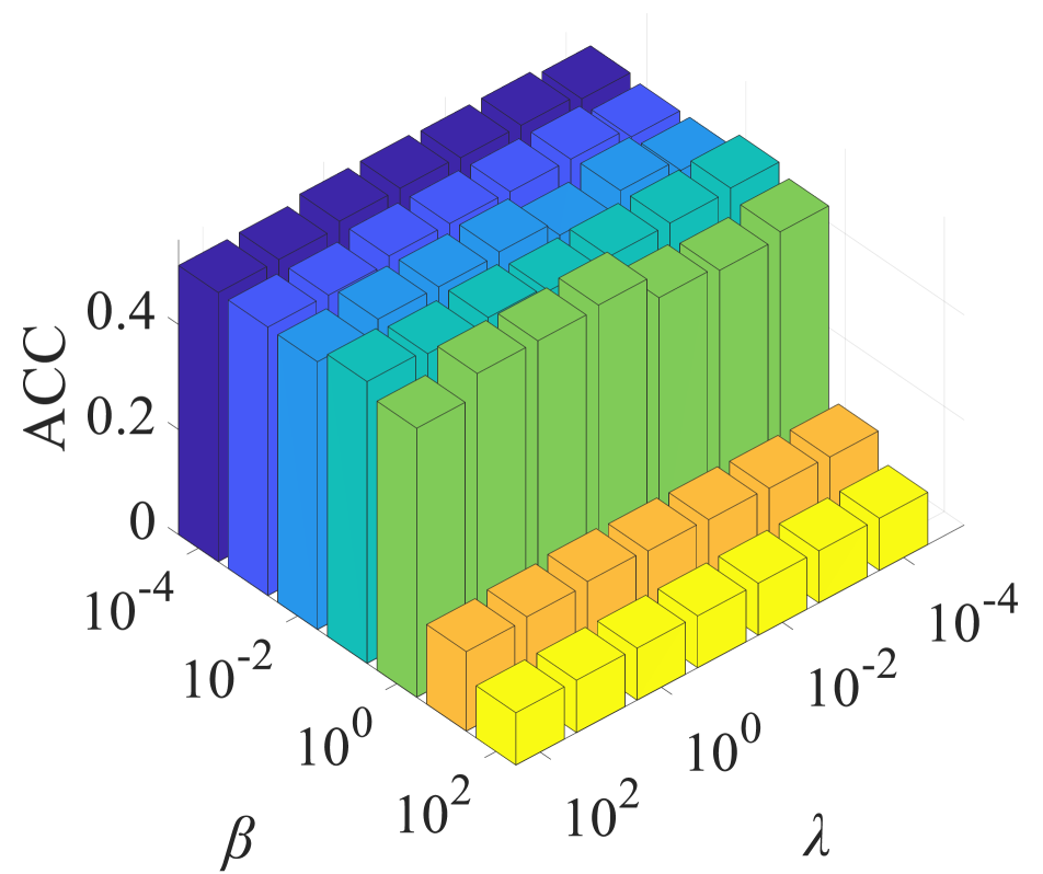
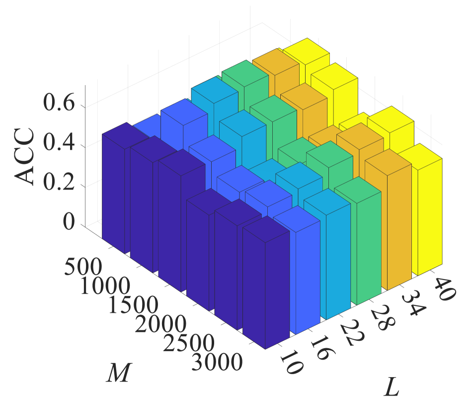
In our experiment, we employed a grid search strategy to determine the optimal choices for all parameters. S2MVTC has a fixed parameter , which is the size of the anchor, and three free parameters: low frequency parameter, denoted as , and two balance parameters, and . We fixed two of these parameters and adjusted the third through an exhaustive search. For instance in dataset Caltech102, we initially fixed and , and adjusted parameters and , where and took values in {, , …, }. The clustering results are shown in Fig. 33(a), where the performance remains stable with in the range of , with ACC close to 55.47%. We observed that the best clustering performance can be achieved within a wide range of , specifically . Additionally, we fixed and , and selected parameter from {500, 1000, …, 3000} and parameter from {10, 16, …, 40}. In Fig. 33(b), performance is stable for within the range, achieving an ACC of approximately 55.47%. Notably, was consistently set to 1000 for all test datasets. To ensure more consistent anchor selection in random sampling, the dataset is sorted in ascending order.
| Methods | ACC | NMI | Purity | F-score | PRE | REC | ARI | CPU Time (s) | Speedup |
| CCV (=0.1, =, =18) | |||||||||
| -means | 0.1339 | 0.0890 | 0.1680 | 0.0930 | 0.0717 | 0.1321 | 0.0201 | 1.12 | 1× |
| BMVC (2018) | 0.2263 | 0.2051 | 0.2612 | 0.1390 | 0.1400 | 0.1380 | 0.0870 | 1.95 | 0.57× |
| SFMC (2020) | 0.1503 | 0.0904 | 0.1562 | 0.1133 | 0.0637 | 0.5105 | 0.0127 | 17.73 | 0.06× |
| OPMC (2021) | 0.1955 | 0.1738 | 0.2309 | 0.1176 | 0.1011 | 0.1407 | 0.0546 | 1.14 | 0.98× |
| FPMVS-CAG (2021) | 0.2284 | 0.1670 | 0.2489 | 0.1333 | 0.1212 | 0.1481 | 0.0749 | 11.62 | 0.10× |
| FMVACC (2022) | 0.1919 | 0.1505 | 0.2308 | 0.1143 | 0.1201 | 0.1091 | 0.0632 | 31.70 | 0.03× |
| FastMICE (2023) | 0.2076 | 0.1623 | 0.2421 | 0.1244 | 0.1264 | 0.1225 | 0.0720 | 17.99 | 0.06× |
| FSMSC (2023) | 0.2167 | 0.1799 | 0.2529 | 0.1273 | 0.1348 | 0.1206 | 0.0773 | 4.50 | 0.25× |
| sMERA-MVC (2023) | 0.4554 | 0.5002 | 0.5191 | 0.3406 | 0.3508 | 0.3310 | 0.3015 | 3.81 | 0.29× |
| S2MVTC | 0.5479 | 0.6119 | 0.5491 | 0.4784 | 0.3871 | 0.6260 | 0.4386 | 1.61 | 0.70X |
| Caltech102 (=1, =10, =16) | |||||||||
| -means | 0.1926 | 0.4083 | 0.3822 | 0.1697 | 0.2390 | 0.2390 | 0.1528 | 40.38 | 1.00× |
| BMVC (2018) | 0.3000 | 0.5096 | 0.4850 | 0.2383 | 0.3496 | 0.1807 | 0.2234 | 7.59 | 5.32× |
| SFMC (2020) | 0.2440 | 0.3216 | 0.2967 | 0.0547 | 0.0288 | 0.5479 | 0.0012 | 59.55 | 0.68× |
| OPMC (2021) | 0.2474 | 0.4848 | 0.4509 | 0.2255 | 0.3456 | 0.1673 | 0.2110 | 31.67 | 1.28× |
| FPMVS-CAG (2021) | 0.3118 | 0.4167 | 0.3786 | 0.2530 | 0.1742 | 0.4652 | 0.2211 | 162.77 | 0.25× |
| FMVACC (2022) | 0.2440 | 0.3216 | 0.2967 | 0.0547 | 0.0288 | 0.5479 | 0.0012 | 57.57 | 0.70× |
| FastMICE (2023) | 0.2408 | 0.4897 | 0.4738 | 0.2042 | 0.3606 | 0.1424 | 0.1913 | 280.79 | 0.14× |
| FSMSC (2023) | 0.2757 | 0.5118 | 0.4974 | 0.2196 | 0.3951 | 0.1521 | 0.2072 | 16.75 | 2.41× |
| sMERA-MVC (2023) | 0.4523 | 0.8053 | 0.7128 | 0.3585 | 0.5858 | 0.2582 | 0.3472 | 58.27 | 0.69× |
| S2MVTC | 0.5547 | 0.8316 | 0.6667 | 0.6577 | 0.6764 | 0.6400 | 0.6481 | 3.56 | 11.34× |
| NUS-WIDE-OBJ (=1, =, =16) | |||||||||
| -means | 0.1227 | 0.1050 | 0.2387 | 0.0849 | 0.1070 | 0.0704 | 0.0390 | 60.04 | 1.00× |
| BMVC (2018) | 0.1573 | 0.1351 | 0.2476 | 0.0972 | 0.1138 | 0.0849 | 0.0483 | 28.19 | 2.13× |
| SFMC (2020) | 0.1330 | 0.0312 | 0.1356 | 0.1132 | 0.0604 | 0.9066 | 0.0005 | 87.09 | 0.69× |
| OPMC (2021) | 0.1438 | 0.1523 | 0.2670 | 0.0973 | 0.1236 | 0.0802 | 0.0524 | 22.56 | 2.66× |
| FPMVS-CAG (2021) | 0.2044 | 0.1338 | 0.2348 | 0.1389 | 0.1124 | 0.1817 | 0.0697 | 75.76 | 0.79× |
| FMVACC (2022) | 0.1226 | 0.1113 | 0.2230 | 0.0765 | 0.1048 | 0.0602 | 0.0341 | 84.44 | 0.71× |
| FastMICE (2023) | 0.1574 | 0.1540 | 0.2611 | 0.1033 | 0.1380 | 0.0825 | 0.0610 | 44.41 | 1.35× |
| FSMSC (2023) | 0.1903 | 0.1326 | 0.2263 | 0.1433 | 0.1164 | 0.1866 | 0.0748 | 30.88 | 1.94× |
| sMERA-MVC (2023) | 0.6135 | 0.8212 | 0.8244 | 0.5996 | 0.7230 | 0.5122 | 0.5786 | 46.15 | 1.30× |
| S2MVTC | 0.6395 | 0.7440 | 0.7329 | 0.6189 | 0.6280 | 0.6101 | 0.5949 | 8.35 | 7.19× |
| AwA (=0.1, =0.03, =9) | |||||||||
| -means | 0.0832 | 0.0951 | 0.0984 | 0.0459 | 0.0366 | 0.0615 | 0.0171 | 802.95 | 1.00× |
| BMVC (2018) | 0.1049 | 0.1253 | 0.1120 | 0.0533 | 0.0510 | 0.0558 | 0.0296 | 32.71 | 24.55× |
| SFMC (2020) | 0.0465 | 0.0288 | 0.0474 | 0.0464 | 0.0238 | 0.9587 | 0.0009 | 129.57 | 6.20× |
| OPMC (2021) | 0.0928 | 0.1193 | 0.1111 | 0.0456 | 0.0449 | 0.0463 | 0.0224 | 182.61 | 4.40× |
| FPMVS-CAG (2021) | 0.0949 | 0.1012 | 0.0997 | 0.0603 | 0.0394 | 0.1282 | 0.0255 | 50.81 | 15.80× |
| FMVACC (2022) | 0.0769 | 0.0906 | 0.0988 | 0.0381 | 0.0403 | 0.0361 | 0.0164 | 640.66 | 1.25× |
| FastMICE (2023) | 0.0905 | 0.1119 | 0.1114 | 0.0458 | 0.0482 | 0.0435 | 0.0241 | 239.61 | 3.35× |
| FSMSC (2023) | 0.1054 | 0.1197 | 0.1259 | 0.0526 | 0.0563 | 0.0493 | 0.0314 | 42.51 | 18.89× |
| sMERA-MVC (2023) | 0.6201 | 0.7820 | 0.6888 | 0.5677 | 0.5479 | 0.5889 | 0.5570 | 390.59 | 2.06× |
| S2MVTC | 0.6288 | 0.8124 | 0.6334 | 0.5872 | 0.4735 | 0.7726 | 0.5748 | 10.35 | 77.58× |
| Cifar-10 (=, =, =16) | |||||||||
| -means | 0.8935 | 0.7849 | 0.8935 | 0.8013 | 0.7976 | 0.8050 | 0.7791 | 111.04 | 1.00× |
| BMVC (2018) | 0.9944 | 0.9846 | 0.9944 | 0.9889 | 0.9889 | 0.9876 | 0.9876 | 12.09 | 9.19× |
| SFMC (2020) | 0.9873 | 0.9671 | 0.9873 | 0.9750 | 0.9750 | 0.9750 | 0.9722 | 119.74 | 0.93× |
| OPMC (2021) | 0.9764 | 0.9420 | 0.9764 | 0.9541 | 0.9540 | 0.9542 | 0.9490 | 21.33 | 5.21× |
| FPMVS-CAG (2021) | 0.8969 | 0.9423 | 0.8972 | 0.8953 | 0.8284 | 0.9796 | 0.8822 | 35.30 | 3.15× |
| FMVACC (2022) | 0.9646 | 0.9627 | 0.9718 | 0.9588 | 0.9489 | 0.9701 | 0.9540 | 134.57 | 0.83× |
| FastMICE (2023) | 0.9920 | 0.9778 | 0.9920 | 0.9842 | 0.9842 | 0.9842 | 0.9824 | 94.05 | 1.18× |
| FSMSC (2023) | 0.9954 | 0.9701 | 0.9663 | 0.9564 | 0.9406 | 0.9744 | 0.9512 | 56.46 | 1.97× |
| sMERA-MVC (2023) | 1.0000 | 1.0000 | 1.0000 | 1.0000 | 1.0000 | 1.0000 | 1.0000 | 214.23 | 0.52× |
| S2MVTC | 0.9994 | 0.9983 | 0.9994 | 0.9989 | 0.9989 | 0.9989 | 0.9988 | 11.13 | 9.98× |
| YoutubeFace_sel (=0.1, =0.005, =19) | |||||||||
| -means | 0.1171 | 0.1025 | 0.2723 | 0.0757 | 0.1068 | 0.0586 | 0.0131 | 1167.73 | 1.00× |
| BMVC (2018) | 0.2815 | 0.2818 | 0.3691 | 0.1169 | 0.1911 | 0.0842 | 0.0658 | 36.12 | 32.33× |
| SFMC (2020) | 0.2843 | 0.0567 | 0.2870 | 0.1665 | 0.0912 | 0.9514 | 0.0039 | 465.44 | 2.51× |
| OPMC (2021) | 0.2574 | 0.2470 | 0.3467 | 0.1139 | 0.1777 | 0.0838 | 0.0600 | 184.88 | 6.32× |
| FMVACC (2022) | 0.2418 | 0.2192 | 0.3329 | 0.0868 | 0.1598 | 0.0596 | 0.0402 | 524.17 | 2.23× |
| FPMVS-CAG (2021) | 0.2510 | 0.2440 | 0.3405 | 0.1305 | 0.1538 | 0.1134 | 0.0591 | 483.83 | 2.41× |
| FastMICE (2023) | 0.3029 | 0.2708 | 0.3859 | 0.1189 | 0.2119 | 0.0826 | 0.0723 | 120.32 | 9.71× |
| FSMSC (2023) | 0.2398 | 0.0332 | 0.2689 | 0.1583 | 0.0895 | 0.6820 | 0.0002 | 174.06 | 6.71× |
| sMERA-MVC (2023) | 0.5381 | 0.6780 | 0.7223 | 0.4279 | 0.6228 | 0.3260 | 0.3906 | 321.29 | 3.63× |
| S2MVTC | 0.5732 | 0.8066 | 0.7943 | 0.4308 | 0.7012 | 0.3109 | 0.3977 | 40.09 | 29.13× |
4.2 Clustering performance analysis
Tab. 3 reports the clustering performance of various methods on six large-scale multi-view datasets, where the best and second-best are highlighted in bold and underlined, respectively. From the table, it is evident that sMERA-MVC and S2MVTC significantly outperform others across various metrics such as ACC, NMI, Purity, F-score, PRE, REC, and ARI. sMERA-MVC, leveraging advanced tensor networks, excels in exploring both inter-view and intra-view correlations of anchor graphs among views simultaneously. This allows sMERA-MVC to utilize the most compact structure for identifying global correlations among anchor graphs, which could be a key factor contributing to its superior performance.
In comparison with sMERA-MVC, S2MVTC consistently outperforms it in most scenarios. Notably, S2MVTC demonstrates a significant improvement in clustering performance on the CCV dataset. For instance, the clustering performance of S2MVTC has shown remarkable enhancements of 9.25%, 11.17%, and 13.71% in terms of ACC, NMI, and ARI, respectively. In the case of the Caltech102, S2MVTC exhibits a performance advantage, achieving a 10.24% higher ACC compared to sMERA-MVC. For the NUS-WIDE-OBJ and AwA datasets, the performances of both methods are similar. Regarding the YoutubeFace_sel dataset, which is larger than other large-scale datasets, sFSR-IMVC demonstrates the best performance compared to sMERA-MVC.
Significantly, in terms of CPU time, , S2MVTC outperforms sMERA-MVC across all large datasets, especially with larger sizes. For instance, it achieves an approximation speedup of 39 times on AwA and 20 times on Cifar-10. Furthermore, BMVC, relying on binary feature representation for clustering, exhibits a CPU time performance at a comparable scale to S2MVTC on large datasets. However, the clustering performance of S2MVTC surpasses BMVC, with ACC improvements of 32.16% on CCV, 25.47% on Caltech102, 48.22% on NUS-WIDE-OBJ, 52.04% on Cifar-10, and 29.18% on YoutubeFace_sel, respectively.
In summary, based on the analysis of these metrics, it can be concluded that the S2MVTC algorithm excels not only in accuracy for multi-view clustering tasks but also significantly outperforms traditional algorithms in terms of computational efficiency, making it suitable for fast large-scale multi-view clustering tasks.
4.3 Model discussions
Model Analysis.
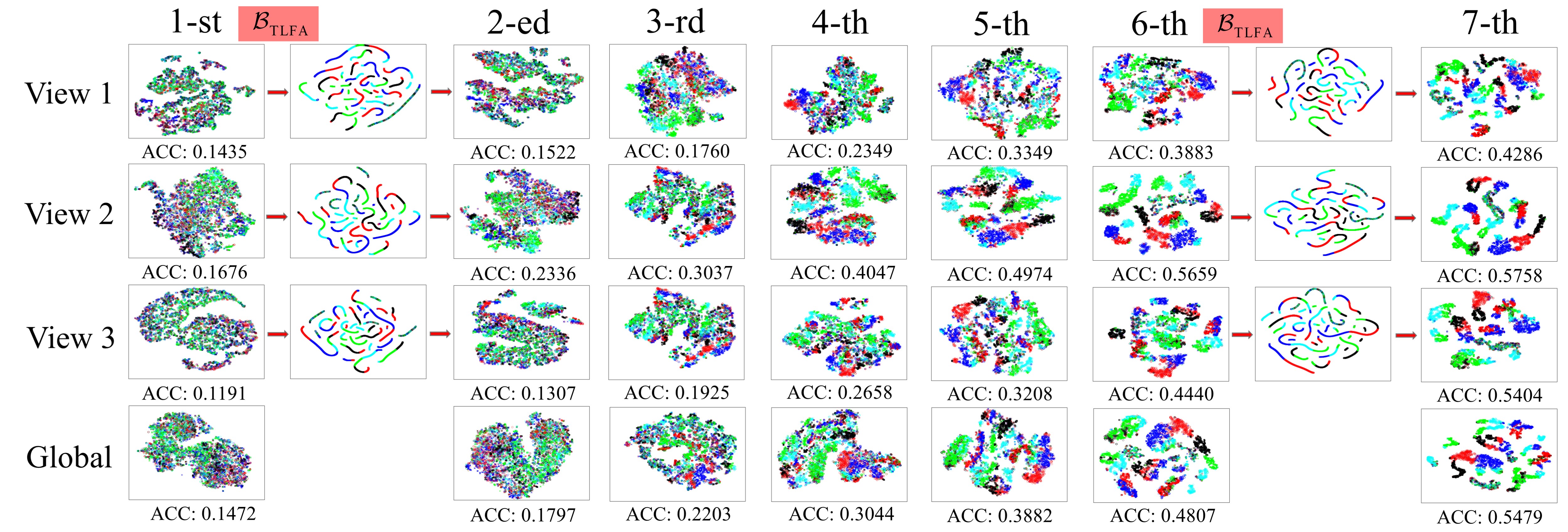
Fig. 4 illustrates the embedding feature learning process of S2MVTC on the CCV dataset.
Compared the 1-st and 3-rd columns, it is evident that after the TLFA operation, the dispersion of sample points increases. This is because that TLFA aims at identifying the compact subspace representation of embedding features across views, known as a smooth representation. During the iterative process, the complementary information captured in this compact subspace further propagates across views. Simultaneously, the exploration of complementary information facilitates the discovery of improved and more smooth subspace representations, ultimately resulting in enhanced clustering performance. For instance, after the 6-th TLFA operation, the clustering performance reaches 54.79%.
Ablation Study. The S2MVTC model consists primarily of three components: 1. Exploration of ISC; 2. Exploration of IGS; 3. Adoption of a nonlinear anchor graph. To further investigate why S2MVTC performs well, we systematically removed each component while keeping the other two fixed, naming these methods as w/o ISC, w/o IGS, and linear anchor graphs. The results are presented in Tab. 4. From the table, it can be observed that removing the exploration of ISC leads to a slight decline in clustering performance, while the removal of the exploration of IGS results in a significant drop in clustering performance. This indicates that the comprehensive exploration of graph similarity among intra-view features effectively, thereby improving clustering performance. Furthermore, when the anchor graph is transformed into a linear mapping between anchors and samples, clustering performance decreases with an increase in the number of samples, especially in Cifar-10 and YoutubeFace_sel. This is because, with a fixed number of anchors, a nonlinear anchor graph is better at capturing relationships between samples when the sample size is exceptionally large.
| w/o ISC | w/o IGS | linear anchor graphs | S2MVTC | |
|---|---|---|---|---|
| Dataset | ACC | ACC | ACC | ACC |
| CCV | 54.42 | 15.49 | 47.31 | 54.79 |
| Caltech102 | 51.31 | 17.27 | 44.71 | 55.47 |
| NUS-WIDE-OBJ | 63.06 | 17.17 | 63.21 | 63.95 |
| AwA | 51.61 | 8.08 | 58.97 | 62.53 |
| Cifar-10 | 99.94 | 65.92 | 88.25 | 99.94 |
| YoutubeFace_sel | 53.97 | 11.38 | 40.20 | 57.33 |
5 Conclusion
In this paper, we present a simple yet efficient scalable multi-view tensor clustering, where the intra-view and inter-view correlations are directly learned from the embedding features. During the iterative process, the introduced TLFA operator optimizes the embedding features to a compact subspace. This optimization aids in exploring complementary information and its propagation across multiple independent views, ensuring maximum consistency between different views. Additionally, we incorporate inter-view semantic consistency and a nonlinear anchor graph to enhance clustering performance. Numerical experiments on six large-scale multi-view datasets demonstrate that our method outperforms all state-of-the-art methods, showcasing a notable improvement with increasing data size.
References
- Baltrušaitis et al. [2018] Tadas Baltrušaitis, Chaitanya Ahuja, and Louis-Philippe Morency. Multimodal machine learning: A survey and taxonomy. TPAMI, 41(2):423–443, 2018.
- Braman [2010] Karen Braman. Third-order tensors as linear operators on a space of matrices. Linear Algebra and its Applications, 433(7):1241–1253, 2010.
- Busch et al. [2023] Erica L Busch, Jessie Huang, Andrew Benz, Tom Wallenstein, Guillaume Lajoie, Guy Wolf, Smita Krishnaswamy, and Nicholas B Turk-Browne. Multi-view manifold learning of human brain-state trajectories. Nature Computational Science, 3(3):240–253, 2023.
- Chen et al. [2022] Man-Sheng Chen, Chang-Dong Wang, and Jian-Huang Lai. Low-rank tensor based proximity learning for multi-view clustering. TKDE, 2022.
- Chen et al. [2023a] Zhe Chen, Xiao-Jun Wu, Tianyang Xu, and Josef Kittler. Fast self-guided multi-view subspace clustering. TIP, pages 1–1, 2023a.
- Chen et al. [2023b] Zhe Chen, Xiao-Jun Wu, Tianyang Xu, and Josef Kittler. Fast self-guided multi-view subspace clustering. TIP, 2023b.
- Chua et al. [July 8-10, 2009] Tat-Seng Chua, Jinhui Tang, Richang Hong, Haojie Li, Zhiping Luo, and Yan-Tao Zheng. Nus-wide: A real-world web image database from national university of singapore. In Proc. of ACM Conf. on Image and Video Retrieval (CIVR’09), Santorini, Greece., July 8-10, 2009.
- Hu et al. [2014] Han Hu et al. Smooth representation clustering. In CVPR, pages 3834–3841, 2014.
- Huang et al. [2023a] Dong Huang, Chang-Dong Wang, and Jian-Huang Lai. Fast multi-view clustering via ensembles: Towards scalability, superiority, and simplicity. TKDE, 35(11):11388–11402, 2023a.
- Huang et al. [2023b] Dong Huang, Chang-Dong Wang, and Jian-Huang Lai. Fast multi-view clustering via ensembles: Towards scalability, superiority, and simplicity. TKDE, 2023b.
- Huster et al. [2012] René J Huster, Stefan Debener, Tom Eichele, and Christoph S Herrmann. Methods for simultaneous eeg-fmri: an introductory review. Journal of Neuroscience, 32(18):6053–6060, 2012.
- Ji and Feng [2023] Jintian Ji and Songhe Feng. Anchor structure regularization induced multi-view subspace clustering via enhanced tensor rank minimization. In ICCV, pages 19343–19352, 2023.
- Jiang et al. [2011] Yu-Gang Jiang, Guangnan Ye, Shih-Fu Chang, Daniel Ellis, and Alexander C. Loui. Consumer video understanding: A benchmark database and an evaluation of human and machine performance. In ICMR, 2011.
- Kang et al. [2020] Zhao Kang, Wangtao Zhou, Zhitong Zhao, Junming Shao, Meng Han, and Zenglin Xu. Large-scale multi-view subspace clustering in linear time. In AAAI, pages 4412–4419, 2020.
- Kilmer et al. [2013] M. Kilmer, K. Braman, N. Hao, and R. Hoover. Third-order tensors as operators on matrices: A theoretical and computational framework with applications in imaging. SIAM J. Matrix Anal. Appl., 34(1):148–172, 2013.
- Kilmer and Martin [2011] Misha E Kilmer and Carla D Martin. Factorization strategies for third-order tensors. Linear Algebra and its Applications, 435(3):641–658, 2011.
- Krizhevsky [2012] Alex Krizhevsky. Learning multiple layers of features from tiny images. 2012.
- Lampert et al. [2014] Christoph H. Lampert, Hannes Nickisch, and Stefan Harmeling. Attribute-based classification for zero-shot visual object categorization. TPAMI, 36(3):453–465, 2014.
- Li et al. [2022a] Fei-Fei Li, Marco Andreeto, Marc’Aurelio Ranzato, and Pietro Perona. Caltech 101, 2022a.
- Li et al. [2020] X. Li, H. Zhang, R. Wang, and F. Nie. Multiview clustering: A scalable and parameter-free bipartite graph fusion method. TPAMI, 44(1):330–344, 2020.
- Li et al. [2022b] Xuelong Li, Han Zhang, Rong Wang, and Feiping Nie. Multiview clustering: A scalable and parameter-free bipartite graph fusion method. TPAMI, 44(1):330–344, 2022b.
- Li et al. [2023] Xingfeng Li, Zhenwen Ren, Quansen Sun, and Zhi Xu. Auto-weighted tensor schatten p-norm for robust multi-view graph clustering. PR, 134:109083, 2023.
- Liu et al. [2021] Jiyuan Liu, Xinwang Liu, Yuexiang Yang, Li Liu, Siqi Wang, Weixuan Liang, and Jiangyong Shi. One-pass multi-view clustering for large-scale data. In ICCV, pages 12344–12353, 2021.
- Long et al. [2023] Zhen Long, Ce Zhu, Jie Chen, Zihan Li, Yazhou Ren, and Yipeng Liu. Multi-view mera subspace clustering. TMM, pages 1–11, 2023.
- Lu et al. [2020] Canyi Lu, Jiashi Feng, Yudong Chen, Wei Liu, Zhouchen Lin, and Shuicheng Yan. Tensor robust principal component analysis with a new tensor nuclear norm. TPAMI, 42(4):925–938, 2020.
- Mulert and Lemieux [2023] Christoph Mulert and Louis Lemieux. EEG-fMRI: physiological basis, technique, and applications. Springer Nature, 2023.
- Recht [2011] Benjamin Recht. A simpler approach to matrix completion. JMLR, 12(12), 2011.
- Rudin et al. [1976] Walter Rudin et al. Principles of mathematical analysis. McGraw-hill New York, 1976.
- Serra et al. [2024] Angela Serra, Paola Galdi, and Roberto Tagliaferri. Multiview learning in biomedical applications. In Artificial intelligence in the age of neural networks and brain computing, pages 307–324. Elsevier, 2024.
- Shu et al. [2022] X. Shu, X. Zhang, Q. Gao, M. Yang, R. Wang, and X. Gao. Self-weighted anchor graph learning for multi-view clustering. TMM, 2022.
- Si et al. [2022] Xiaomeng Si, Qiyue Yin, Xiaojie Zhao, and Li Yao. Consistent and diverse multi-view subspace clustering with structure constraint. PR, 121:108196, 2022.
- Sun [2013] Shiliang Sun. A survey of multi-view machine learning. Neural computing and applications, 23:2031–2038, 2013.
- Van der Maaten and Hinton [2008] Laurens Van der Maaten and Geoffrey Hinton. Visualizing data using t-sne. JMLR, 9(11), 2008.
- Von Luxburg [2007] U. Von Luxburg. A tutorial on spectral clustering. Statistics and computing, 17(4):395–416, 2007.
- Wang et al. [2023] Huibing Wang, Mingze Yao, Guangqi Jiang, Zetian Mi, and Xianping Fu. Graph-collaborated auto-encoder hashing for multiview binary clustering. TNNLS, pages 1–13, 2023.
- Wang et al. [2022a] Nan Wang, Dongren Yao, Lizhuang Ma, and Mingxia Liu. Multi-site clustering and nested feature extraction for identifying autism spectrum disorder with resting-state fmri. Medical image analysis, 75:102279, 2022a.
- Wang et al. [2021] S. Wang, X. Liu, X. Zhu, P. Zhang, Y. Zhang, F. Gao, and E. Zhu. Fast parameter-free multi-view subspace clustering with consensus anchor guidance. TKDE, 31:556–568, 2021.
- Wang et al. [2022b] Siwei Wang, Xinwang Liu, Suyuan Liu, Jiaqi Jin, Wenxuan Tu, Xinzhong Zhu, and En Zhu. Align then fusion: Generalized large-scale multi-view clustering with anchor matching correspondences. NeurIPS, 35:5882–5895, 2022b.
- Wang et al. [2022c] Siwei Wang, Xinwang Liu, Xinzhong Zhu, Pei Zhang, Yi Zhang, Feng Gao, and En Zhu. Fast parameter-free multi-view subspace clustering with consensus anchor guidance. TIP, 31:556–568, 2022c.
- Wen et al. [2021] J. Wen, Z. Zhang, Z. Zhang, L. Zhu, L. Fei, B. Zhang, and Y. Xu. Unified tensor framework for incomplete multi-view clustering and missing-view inferring. In Proc. AAAI Conf. Artif. Intell., pages 10273–10281, 2021.
- Wolf et al. [2011] Lior Wolf, Tal Hassner, and Itay Maoz. Face recognition in unconstrained videos with matched background similarity. In CVPR, 2011.
- Xia et al. [2022] W. Xia, Q. Gao, Q. Wang, X. Gao, C. Ding, and D. Tao. Tensorized bipartite graph learning for multi-view clustering. TPAMI, 2022.
- Yang et al. [2022] M. Yang, P. Li, Y.and Hu, J. Bai, J. Lv, and X. Peng. Robust multi-view clustering with incomplete information. TPAMI, 45(1):1055–1069, 2022.
- Zhang et al. [2022] Yachao Zhang, Yuan Xie, Cuihua Li, Zongze Wu, and Yanyun Qu. Learning all-in collaborative multiview binary representation for clustering. TNNLS, pages 1–14, 2022.
- Zhang et al. [2018] Zheng Zhang, Li Liu, Fumin Shen, Heng Tao Shen, and Ling Shao. Binary multi-view clustering. TPAMI, 41(7):1774–1782, 2018.