SAD: Semi-Supervised Anomaly Detection on Dynamic Graphs
Abstract
Anomaly detection aims to distinguish abnormal instances that deviate significantly from the majority of benign ones. As instances that appear in the real world are naturally connected and can be represented with graphs, graph neural networks become increasingly popular in tackling the anomaly detection problem. Despite the promising results, research on anomaly detection has almost exclusively focused on static graphs while the mining of anomalous patterns from dynamic graphs is rarely studied but has significant application value. In addition, anomaly detection is typically tackled from semi-supervised perspectives due to the lack of sufficient labeled data. However, most proposed methods are limited to merely exploiting labeled data, leaving a large number of unlabeled samples unexplored. In this work, we present semi-supervised anomaly detection (SAD), an end-to-end framework for anomaly detection on dynamic graphs. By a combination of a time-equipped memory bank and a pseudo-label contrastive learning module, SAD is able to fully exploit the potential of large unlabeled samples and uncover underlying anomalies on evolving graph streams. Extensive experiments on four real-world datasets demonstrate that SAD efficiently discovers anomalies from dynamic graphs and outperforms existing advanced methods even when provided with only little labeled data.
1 Introduction
Anomaly detection, which identifies outliers (called anomalies) that deviate significantly from normal instances, has been a lasting yet active research area in various research contexts Ma et al. (2021). In many real-world scenarios, instances are often explicitly connected with each other and can be naturally represented with graphs. Over the past few years, anomaly detection based on graph representation learning has emerged as a critical direction and demonstrated its power in detecting anomalies from instances with abundant relational information. For example, in a financial transaction network where fraudsters would try to cheat normal users and make illegal money transfers, the graph patterns captured from the local and global perspectives can help detect these fraudsters and prevent financial fraud.
In real-world scenarios, it is often challenging to tackle the anomaly detection problem with supervised learning methods since annotated labels in most situations are rare and difficult to acquire. Therefore, current works mainly focus on unsupervised schemes to perform anomaly detection, with prominent examples including autoencoders Zhou and Paffenroth (2017), adversarial networks Chen et al. (2020), or matrix factorization Bandyopadhyay et al. (2019). However, they tend to produce noisy results or uninterested noise instances due to insufficient supervision. Empirically, it is usually difficult to get desired outputs from unsupervised methods without the guidance of precious labels or correct assumptions.
Semi-supervised learning offers a principled way to resolve the issues mentioned above by utilizing few-shot labeled data combined with abundant unlabeled data to detect underlying anomalies Ma et al. (2021). Such methods are practical in real-world applications and can definitely obtain much better performance than fully unsupervised methods when the labeled data is leveraged properly. In recent years, a vast majority of work adopts graph-based semi-supervised learning models for solving anomaly detection problems, resulting in beneficial advances in anomaly analytics techniques Pang et al. (2019); Ding et al. (2021); Qian et al. (2021).
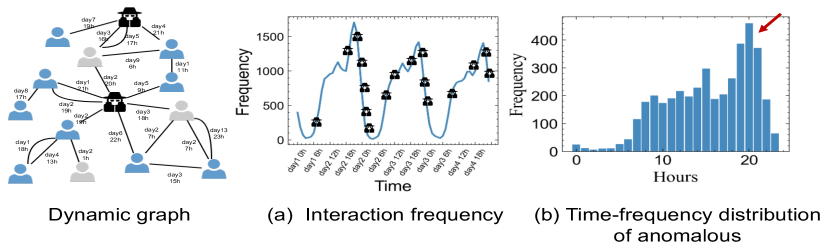
Yet, there are still two fundamental limitations to these existing semi-supervised anomaly detection methods: (1) Underutilization of unlabeled data. Although existing semi-supervised approaches have utilized labeled data to perform anomaly detection, few methods take advantage of large-scale unlabeled samples that contain a lot of useful information. As a result, they suffer poor performance particularly when limited labels are provided. (2) Lack of dynamic information mining. In practice, graphs are dynamic in nature, with nodes, edges, and attributes evolving constantly over time. Such characteristics may be beneficial in solving anomaly detection problems. As shown in Figure 1, the behavioral statistics of users show certain cyclical patterns in the time domain, which can be directly captured by dynamic graph neural networks. To our best knowledge, most previous attempts mainly focus on static graphs which neglect temporal information, such design has proven to be sub-optimal in dynamic graph scenario Liu et al. (2021). Although there are some recent efforts Meng et al. (2021); Liu et al. (2021)have explored ways to combine dynamic information in their work, they simply incorporate time as a feature in the model, leading to insufficient temporal information modeling and degraded performance on anomaly detection.
In this work, we propose a novel semi-supervised anomaly detection (SAD) framework that tackles the aforementioned limitations. The proposed framework first utilizes a temporal graph network to encode graph data for both labeled and unlabeled samples, followed by an anomaly detector network to predict node anomaly scores. Then, a memory bank is adopted to record each predicted anomaly score together with node time information, to produce a normal sample statistical distribution as prior knowledge and guide the learning of the network subsequently by using a deviation loss. In order to further exploit the potential of large unlabeled data, we introduce a novel pseudo-label contrastive learning module, which leverages the predicted anomaly scores to form pseudo-groups by calculating score distance between nodes - nodes with closer distance will be classified into the same pseudo-group, nodes within the same pseudo-group will form positive pairs for contrastive learning.
Our main contributions are summarized as follows:
-
•
We propose SAD, an end-to-end semi-supervised anomaly detection framework, which is tailored with a time-equipped memory bank and a pseudo-label contrastive learning module to effectively solve the anomaly detection problem on dynamic graphs.
-
•
Our proposed SAD framework uses the statistical distribution of unlabeled samples as the reference distribution for loss calculation and generates pseudo-labels correspondingly to participate in supervised learning, which in turn fully exploits the potential of unlabeled samples.
-
•
Extensive experiments demonstrate the superiority of the proposed framework compared to strong baselines. More importantly, our proposed approach can also significantly alleviate the label scarcity issue in practical applications.
2 Related Work
2.1 Dynamic Graph Neural Networks
Graph neural networks (GNNs) have been prevalently used to represent structural information from graph data. However, naive applications of static graph learning paradigms Hamilton et al. (2017); Velickovic et al. (2018) in dynamic graphs fail to capture temporal information and show up as suboptimal in dynamic graph scenarios Xu et al. (2020a). Thus, some methods Singer et al. (2019); Pareja et al. (2020) model the evolutionary process of a dynamic graph by discretizing time and reproducing multiple static graph snapshots. Such a paradigm is often infeasible for real-world systems that need to handle each interaction event instantaneously, in which graphs are represented by a continuous sequence of events, i.e., nodes and edges can appear and disappear at any time.
Some recent work has begun to consider the direct modeling of temporal information and proposed a continuous time dynamic graph modeling scheme. For example, DyREP Trivedi et al. (2019) uses a temporal point process model, which is parameterized by a recurrent architecture to learn evolving entity representations on temporal knowledge graphs. TGAT Xu et al. (2020a) proposes a novel functional time encoding technique with a self-attention layer to aggregate temporal-topological neighborhood features. However, the above methods rely heavily on annotated labels, yet obtaining sufficient annotated labels is usually very expensive, which greatly limits their application in real-world scenarios such as anomaly detection.
2.2 Anomaly Detection with GNNs
Anomalies are rare observations (e.g., data records or events) that deviate significantly from the others in the sample, and graph anomaly detection (GAD) aims to identify anomalous graph objects (i.e., nodes, edges, or sub-graphs) in a single graph as well as anomalous graphs among a set/database of graphs Ma et al. (2021). The anomaly detection with GNNs is mainly divided into unsupervised and semi-supervised methods. Unsupervised anomaly detection methods are usually constructed with a two-stage task, where a graph representation learning task is first constructed, and then abnormality measurements are applied based on the latent representations Akoglu et al. (2015). Rader Li et al. (2017) detects anomalies by characterizing the residuals of the attribute information and their correlation with the graph structure. Autoencoder Zhou and Paffenroth (2017) learns graph representations through an unsupervised feature-based deep autoencoder model. DOMINANT Ding et al. (2019) uses a GCN-based autoencoder framework that uses reconstruction errors from the network structure and node representation to distinguish anomalies. CoLA Liu et al. (2022) proposes a self-supervised contrastive learning method based on capturing the relationship between each node and its neighboring substructure to measure the agreement of each instance pair.
A more recent line of work proposes employing semi-supervised learning by using small amounts of labeled samples from the relevant downstream tasks to address the problem that unsupervised learning tends to produce noisy instances. SemiGNN Wang et al. (2019) learn a multi-view semi-supervised graph with hierarchical attention for fraud detection. GDN Ding et al. (2021) adopts a deviation loss to train GNN and uses a cross-network meta-learning algorithm for few-shot node anomaly detection. SemiADC Meng et al. (2021) simultaneously explores the time-series feature similarities and structure-based temporal correlations. TADDY Liu et al. (2021) constructs a node encoding to cover spatial and temporal knowledge and leverages a sole transformer model to capture the coupled spatial-temporal information. However, these methods are based on discrete-time snapshots of dynamical graphs that are not well suited to continuous time dynamical graphs, and the temporal information is simply added to the model using a linear network mapping as features, without taking into account temporal properties such as periodicity.
3 PRELIMINARIES
3.1 Notations and Problem Formulation
Notations. Continuous-time dynamic graphs are important for modeling relational data for many real-world complex applications. The dynamic graph can be represented as , where is the set of nodes involved in all temporal events, and denotes a sequence of temporal events. Typically, let be an event stream that generates the temporal network and is the number of observed events, with an event indicating an interaction or a link happens from source node to target node at time , with associating edge feature . Note that there might be multiple links between the same pair of node identities at different timestamps.
Problem formulation. In practical applications, it is very difficult to obtain large-scale labeled data due to the prohibitive cost of collecting such data. The goal of our work is to be able to improve the performance of anomaly detection based on very limited supervised knowledge. Taking the task of temporal event anomaly detection as an example, based on a dynamic graph , we assume that each event has a corresponding true label . However, due to the limitation of objective conditions, only a few samples of the label can be observed, denoted by , and the rest are unlabeled data denoted by . In our problem , our task is to learn an anomaly score mapping function that separates abnormal and normal samples.
4 Method
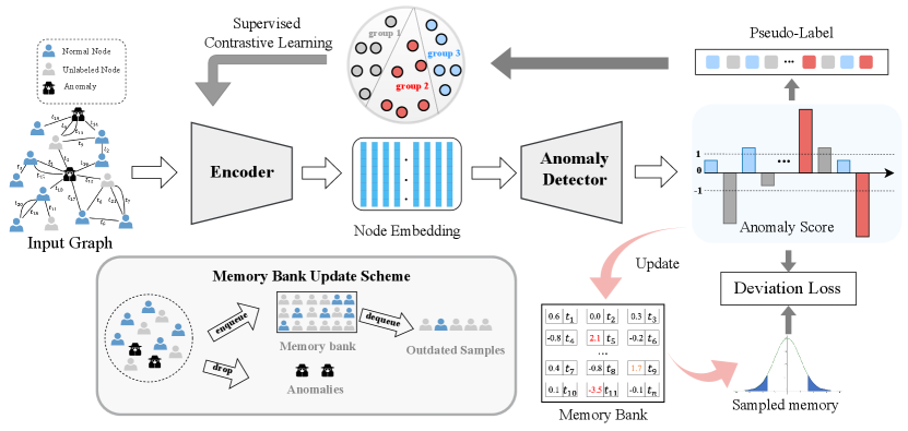
In this section, we detail the components of the proposed framework SAD for anomaly detection on dynamic graphs. As shown in Figure 2, the overall structure of SAD consists of the following main components: a temporal graph encoder that produces node embeddings (Section 4.1), the combination of an anomaly detector and a time-equipped memory bank to distinguish anomalous samples using prior knowledge of unlabeled data (Section 4.1), and a supervised contrastive learning module can yield pseudo-labeling to mine the potential of unlabeled data (Section 4.2). We also detail several strategies for parameter learning under our framework (Section 4.3).
4.1 Deviation Networks with Memory Bank
To enable anomaly detection with few-shot labeled data, we construct a graph deviation network following Ding et al. (2021). However, for application to dynamic graphs, we first use a temporal graph encoder based on temporal encoding information to learn node representations and additionally construct a memory bank to dynamically record the overall statistical distribution of normal and unlabeled samples as a reference score to calculate the deviation loss that optimizes the model with few-shot labeled samples. The entire deviation network is semi-supervised, with abundant unlabeled samples used as statistical priors in the memory bank and few-shot labeled data used for calculating deviation losses.
Temporal graph encoder. Since dynamic graphs contain information about the time differences of edges, we first deploy a temporal graph encoder as a node embedding module to learn the topology of the graph by mapping nodes to a low-dimensional latent representation. The graph encoder is multiple GNN layers that take the graph constructed at time as input and extract node representations for all in through the message-passing mechanism. Formally, the forward propagation at -th layer is described as follows:
| (1) | ||||
where is the intermediate representations of node in the -th layer at the timestamp and denotes the set of first-order neighboring nodes of the node occurred prior to . is the associating edge feature between and , represents the relative timespan of two timestamps, and is a relative time encoder based on the cosine transform mentioned in Xu et al. (2020a), which implements a functional time projection from the time domain to the continuous space and helps to capture the periodic patterns on the dynamic graph. is an aggregation function for propagating and aggregating messages from neighborhoods, followed by a function for combining representations from neighbors and its previous-layer representation. Note that the and functions in our framework can be flexibly designed for different applications without any constraints. Finally, we can obtain the node embedding of node with the -th aggregation layer. In practice, across all tasks, we adopt TGAT as the temporal graph encoder.
Anomaly Detector. To distinguish abnormal samples from normal samples, we introduce an anomaly detector to map the learned node embedding to an anomaly score space, where normal samples are clustered and abnormal samples deviate from the set. Specifically, we use a simple feed-forward neural network as the anomaly detector:
| (2) |
where , , and are learnable parameters of the anomaly detector. In our framework, is a one-dimensional anomaly score with a value range from to . Ideally, the anomaly scores of normal samples are clustered in a certain interval, and it is easy to find out the anomalies (outliers) based on the overall distribution of the anomaly scores.
Memory bank. In essence, the task of SAD is to discriminate anomalous nodes from large-scale normal/unlabeled nodes in the dynamic graph utilizing a few labeled samples. The anomaly scores of normal nodes are clustered together in the anomaly score space after training with the optimization objective (which will be introduced later), while the anomaly scores of the anomaly samples will deviate from the overall distribution. Hence, we generate this distribution by using a memory bank to record the historical anomaly scores of unlabeled and normal samples, based on the assumption that most of the unlabeled data are normal samples. The messages that need to be stored in the memory bank are described as the following:
| (3) |
where is the label information of node at timestamp and its value and represent that the node is an unlabeled or normal sample at the current timestamp, respectively.
Note that the attribute of the nodes in the dynamic graph evolves continuously, with consequent changes in the labels and anomaly scores. Perceptually, samples with longer time intervals should have less influence on the current statistical distribution, so we also record the corresponding time t for each anomaly score in the memory bank.
| (4) |
Meanwhile, the memory bank is designed as a first-in-first-out (FIFO) queue of size . The queue size is controlled by discarding samples that are sufficiently old since outdated samples yield less gain due to changes in model parameters during the model training process.
Deviation loss. Inspired by the recent success of deviation networks Pang et al. (2019); Ding et al. (2021), we adopt deviation loss as our main learning objective to enforce the model to separate out normal nodes and abnormal nodes whose characteristics significantly deviate from normal nodes in the anomaly score space. Different from their methods, we use a memory bank to produce a statistical distribution of normal samples instead of using a standard normal distribution as the reference score. This takes into account two main factors, one is that statistical distribution generated by real anomaly score can better show the properties of different datasets, and the other is that in dynamic graphs, the data distribution can fluctuate more significantly due to realistic situations such as important holidays or periodic events, so it is not suitable to use a simple standard normal distribution as the reference distribution of normal samples.
To obtain the reference score in the memory bank, we assume that the distribution of the anomaly score satisfies the Gaussian distribution, which is a very robust choice to fit the anomaly scores of various datasets Kriegel et al. (2011). Based on this assumption, we randomly sample a set of examples from the memory bank for calculating the reference score, which helps to improve the robustness of the model by introducing random perturbations. Meanwhile, we introduce the effect of time decay and use the relative timespan between the timestamp and the anomaly score storage time to calculate the weighting term for each statistical example . The reference scores (mean and standard deviation ) of the normal sample statistical distribution at the timestamp are calculated as follows:
| (5) | ||||
With the reference scores at the timestamp , we define the deviation between the anomaly score of node and the reference score in the following:
| (6) |
The final deviation loss is then obtained by plugging deviation into the contrast loss Hadsell et al. (2006) as follows:
| (7) |
where is the label information of node at timestamp and is equivalent to a Z-Score confidence interval parameter. Note that in this semi-supervised task, only labeled samples are directly involved in computing the objective function. Optimizing this loss will enable the anomaly score of normal samples as close as possible to the overall distribution in the memory bank, while the anomaly scores of anomalies are far from the reference distribution.
4.2 Contrastive Learning for Unlabeled Samples
To fully exploit the potential of unlabeled samples, we generate a pseudo-label for each sample based on the existing deviation scores and involve them in the training of the graph encoder network. Here, we design a supervised contrastive learning task such that nodes with closer deviation scores also have more similar node representations, while nodes with larger deviation score differences have larger differences in their corresponding representations. The goal of this task is consistent with our deviation loss, which makes the difference between normal and anomaly samples deviate in both the representation space and anomaly score space. For a batch training sample with batch size , we first obtain the deviation distance between any two samples and . On the standard normal distribution anomaly space, we group nodes with intervals less than into the same class. Thus, for a single sample , its supervised contrastive learning loss takes the following form:
| (8) |
where is a scalar temperature parameter, and denotes similarity weights between positive sample pairs. The final objective function is the sum of the losses of all nodes: .
4.3 Learning procedure
For anomaly detection tasks, the optimization of the whole network is based on deviation loss and contrastive learning loss. Noted that the contrastive learning loss is only used to train the parameters of the temporal graph encoder. Specifically, let denote all the parameters of the temporal graph encoder, and denote the learnable parameters in the anomaly detector. The optimization task of our model is as follows:
| (9) |
where is a hyperparameter for balancing the contribution of contrastive learning loss.
In addition to anomaly detection tasks, we also present an end-to-end learning procedure to cope with different downstream tasks. Taking the downstream task of node classification as an example, in order to obtain the score results for node classification, we use a simple multi-layer perception (MLP) as the projection network to learn the classification results based on the node representations after the graph encoder. Let denote the learnable parameters in the projection network. Assume that the downstream supervised task with loss function , the optimization task of our model is as follows:
| (10) |
where and are hyperparameters for balancing the contributions of two losses.
| Wikipedia | Mooc | Alipay | ||
| #Nodes | 9,227 | 10,984 | 7,074 | 3,575,301 |
| #Edges | 157,474 | 672,447 | 411,749 | 53,789,768 |
| #Edge features | 172 | 172 | 4 | 100 |
| #Anomalies | 217 | 366 | 4,066 | 24,979 |
| Timespan | 30 days | 30 days | 30 days | 90 days |
| Pos. label meaning | posting banned | editing banned | dropping out | fraudster |
| Chronological Split | 70%-15%-15% | 70%-15%-15% | 70%-15%-15% | 70%-15%-15% |
5 Experiments
5.1 Experimental Setup
Datasets. In this paper, we use four real-world datasets, including three public bipartite interaction dynamic graphs and an industrial dataset. Wikipedia Kumar et al. (2019) is a dynamic network tracking user edits on wiki pages, where an interaction event represents the page edited by the user. Dynamic labels indicate whether a user is banned from posting. Reddit Kumar et al. (2019) is a dynamic network tracking active users posting in subreddits, where an interaction event represents a user posting on a subreddit. The dynamic binary labels indicate if a user is banned from posting under a subreddit. MOOC Kumar et al. (2019) is a dynamic network tracking students’ actions on MOOC online course platforms, where an interaction event represents user actions on the course activity. The Alipay dataset is a dynamic financial transaction network collected from the Alipay platform, and dynamic labels indicate whether a user is a fraudster. Note that the Alipay dataset has undergone a series of data-possessing operations, so it cannot represent real business information. For all tasks and datasets, we adopt the same chronological split with 70% for training and 15% for validation and testing according to node interaction timestamps. The statistics are summarized in Table 1.
Implementation details. Regarding the proposed SAD model, we use a two-layer, two-head TGAT Xu et al. (2020a) as a graph network encoder to produce 128-dimensional node representations. For model hyperparameters, we fix the following configuration across all experiments without further tuning: we adopt Adam as the optimizer with an initial learning rate of 0.0005 and a batch size of 256 for both training. We adopt mini-batch training for SAD and sample two-hop subgraphs with 20 nodes per hop. For the memory bank, we set the memory size as 4000, and the sampled size as 1000. To better measure model performance in terms of AUC metrics, we choose the node classification task (similar to anomaly node detection) as the downstream task, so we adopt Eq.(10) as the model optimization objective and find that pick and performs well across all datasets. The proposed method is implemented using PyTorch Paszke et al. (2019) 1.10.1 and trained on a cloud server with NVIDIA Tesla V100 GPU. Code is made publicly available at https://github.com/D10Andy/SAD for reproducibility.
| Methods | Wikipedia | Mooc | Alipay | |
|---|---|---|---|---|
| TGAT | 83.23 0.84 | 67.06 0.69 | 66.88 0.68 | 92.53 0.93 |
| TGN | 84.67 0.36 | 62.66 0.85 | 67.07 0.73 | 92.84 0.81 |
| Radar | 82.91 0.97 | 61.46 1.27 | 62.14 0.89 | 88.18 1.05 |
| DOMINANT | 85.84 0.63 | 64.66 1.29 | 65.41 0.72 | 91.57 0.93 |
| SemiGNN | 84.65 0.82 | 64.18 0.78 | 64.98 0.63 | 92.29 0.85 |
| GDN | 85.12 0.69 | 67.02 0.51 | 66.21 0.74 | 93.64 0.79 |
| TADDY | 84.72 1.01 | 67.95 0.94 | 68.47 0.76 | 93.15 0.88 |
| SAD | 86.77 0.24 | 68.77 0.75 | 69.44 0.87 | 94.48 0.65 |
5.2 Overall Performance
We compare our SAD against several strong baselines of graph anomaly detection methods on node classification tasks, the baselines in our experiments include our backbone model TGAT and the state-of-the-art supervised learning method TGN-no-mem Xu et al. (2020b), as well as five graph anomaly detection methods, which are specifically divided into unsupervised anomaly detection methods (Radar and DOMINANT) and semi-supervised anomaly detection methods (SemiGNN, GDN, and TADDY). In order to be able to fairly compare the performance of the different methods, we use the same structure of the projection network to learn the classification results based on the node embedding outputted by their anomaly detection tasks. Table 2 summarizes the dynamic node classification results on different datasets. For all experiments, we report the average results with standard deviations of 10 different runs.
As shown in Table 2, our approach outperforms all baselines on all datasets. Due to the lack of dynamic information, these static graph anomaly detection methods (Radar, SemiGNN, DOMINANT, and GDN) perform worse than the dynamic graph supervision model TGAT on Reddit and Mooc, which are more sensitive to temporal information. On these datasets with large differences in the proportion of positive and negative samples, our method shows a significant improvement compared to TGAT. Specifically, the relative average AUC value improvements on Wikipedia, Reddit, Mooc, and Alipay are , , , and , respectively. Compared with the recent dynamic graph anomaly detection method TADDY, our method improves , , , and on four datasets, respectively. We believe the significant improvements are that SAD captures more information on time-decaying state changes and that the memory bank mechanism can effectively obtain the distribution of normal data, which helps to detect anomaly samples.
5.3 Few-shot Evaluation
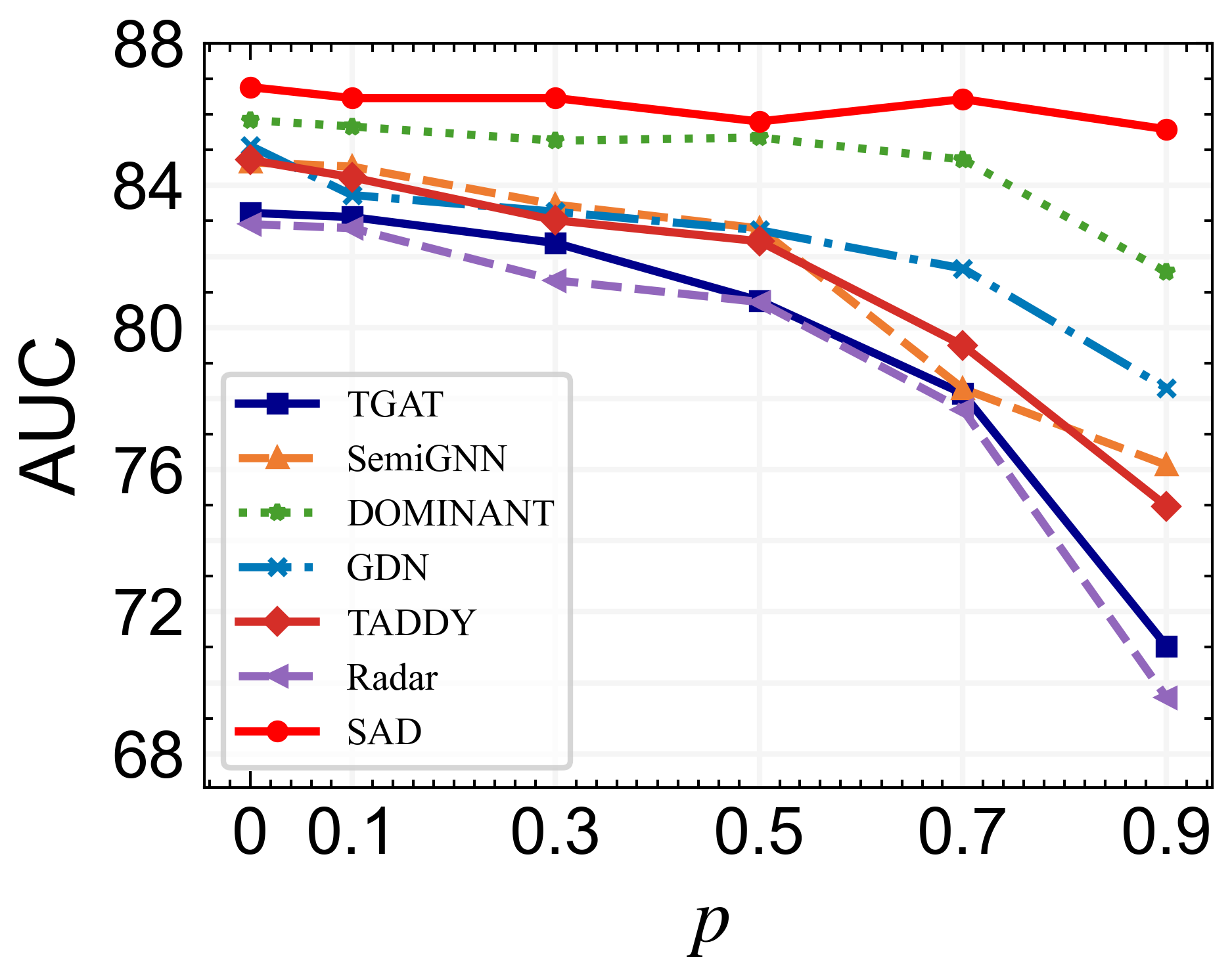
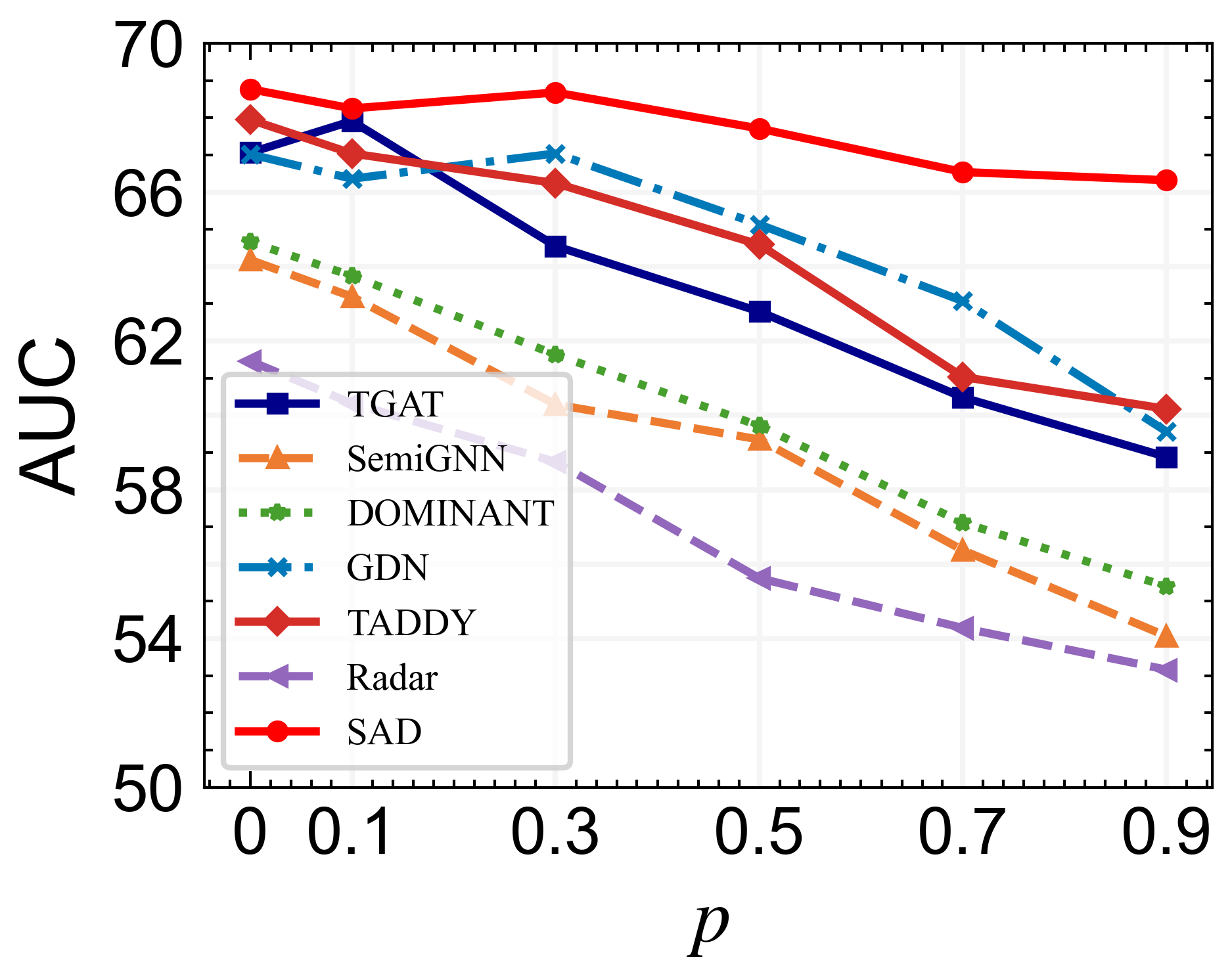
The training samples used in the overall performance are annotated. However, in real application scenarios, annotated samples are always difficult to obtain, and anomaly detection algorithms need to be applied to distinguish anomalous nodes in large-scale unlabeled samples. To thoroughly evaluate the benefits of different graph anomaly detection approaches in few-shot scenarios, we varied the drop rate , i.e., the ratio of randomly removed node labels in the training set, from to with a step size of .
The curve of AUC values of different models and datasets along with the label drop ratio is drawn in Figure 3. SAD achieves state-of-the-art performance in all cases across two dynamic datasets. Noticeably, we observe that SAD achieves optimal performance on both datasets when the drop rate is at . The result indicates that there is a lot of redundant or noisy information in the current graph datasets, which easily leads to overfitting of the model training. By dropping this part of label information and using pseudo-labeled data to participate in the training, the performance of the model is improved instead. Other methods have a significant degradation in performance at a drop ratio of . Nevertheless, SAD still outperforms all the baselines by a large margin on two datasets, and the downstream performance is not significantly sacrificed even for a particular large dropping ratio (e.g., 0.7 and 0.9). This indicates that even for few-shot scenarios, SAD could still mine useful statistical information for downstream tasks and distinguish anomalous nodes with information from abundant unlabeled samples. Overall, we believe that the performance improvement in our model comes from two reasons: one is that the memory bank-dominated anomaly detector allows the model to learn a discriminative representation between normal and anomalous samples, and the other is that contrastive learning based on pseudo labels helps to learn generic representations of nodes even in the presence of large amounts of unlabeled data.
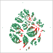
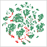
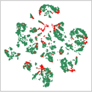
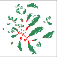
5.4 Visualization Analysis
In this part, we visualize the learned node embeddings to evaluate the proposed method. And the 2D t-SNE van der Maaten and Hinton (2008) is used to reduce the dimensions of the hidden layer output node embeddings from 128 to 2. Figure 4 shows the visualization of node embeddings learned by TGAT, GDN, TADDY, and SAD on Alipay. As we can see, the node embeddings of SAD are able to separate the abnormal and normal samples well. The supervised learning method TGAT is prone to overfitting during training on datasets with class imbalance, resulting in poor discrimination of node representation learning. GDN is not effective in learning node embedding because it does not take into account dynamic information and historical data statistical distributions. TADDY is based on modeling discrete-time snapshots of dynamical graphs that are not well suited to continuous-time dynamical graphs. Overall, these results show that the proposed method can learn useful node embeddings for anomaly detection tasks on dynamic graphs.
5.5 Ablation Study
Finally, we conduct an ablation study to better examine the contribution of different components in the proposed framework, detailed as follows:
-
•
backbone. This entity indicates that only the graph coding network is used for dynamic node classification tasks in a supervised learning manner.
-
•
w/dev. This variant indicates that the deviation network based on standard normal distribution is used on the basis of the backbone model, without the memory bank mechanism.
-
•
w/mem. This variant indicates that the memory bank mechanism without the time decay technique is used on the basis of the w/dev model.
-
•
w/time. This variant indicates that the time decay technique in the memory bank is used on the basis of the w/mem model.
-
•
w/scl. This variant indicates that the supervised contrastive learning module is used on the basis of the w/time model, which corresponds to our full model.
| Wikipedia | Mooc | ||
|---|---|---|---|
| TGAT | 80.76 2.30 | 62.79 3.42 | 64.04 1.02 |
| w/dev | 82.45 0.64 | 64.15 2.93 | 65.33 1.67 |
| w/mem | 85.20 1.30 | 66.96 1.51 | 67.25 0.75 |
| w/time | 85.44 0.75 | 66.78 1.98 | 67.53 0.93 |
| w/scl | 85.80 1.32 | 67.71 0.75 | 67.57 0.54 |
To verify the performance of the model in a large number of unlabeled sample scenarios, we manually drop of the labels of the training set at random. Table 3 present the results given by our several sub-modules. We summarize our observations as follows: Firstly, each of the incremental submodules proposed in our paper helps to improve the performance of the model. Among them, the memory bank mechanism yields the largest performance improvements, e.g., , , and performance improvement on Wikipedia, Reddit, and Mooc, respectively. Secondly, the complete model outperforms the base model on the three dynamic datasets by , , and , respectively, which verifies the effectiveness of the proposed submodule by introducing the deviation loss and contrastive learning based on pseudo labels.
6 Conclusion
We present a semi-supervised learning framework SAD for detecting anomalies over dynamic graphs. The proposed framework utilizes a temporal graph network and an anomaly detector to learn the anomaly score and uses a time-equipped memory bank to record the overall statistical distribution of normal and unlabeled samples as prior knowledge to guide the subsequent learning of the model in a semi-supervised manner. To further explore the potential of unlabeled samples, we produce pseudo-labels based on the difference between the anomaly scores and use these labels directly to train the backbone network in a supervised contrastive learning manner. Our results from extensive experiments demonstrate that the proposed SAD can achieves competitive performance even with a small amount of labeled data.
References
- Akoglu et al. [2015] Leman Akoglu, Hanghang Tong, and Danai Koutra. Graph based anomaly detection and description: a survey. Data Min. Knowl. Discov., 29(3):626–688, 2015.
- Bandyopadhyay et al. [2019] Sambaran Bandyopadhyay, N. Lokesh, and M. Narasimha Murty. Outlier aware network embedding for attributed networks. In The Thirty-Third AAAI Conference on Artificial Intelligence, AAAI 2019, The Thirty-First Innovative Applications of Artificial Intelligence Conference, IAAI 2019, The Ninth AAAI Symposium on Educational Advances in Artificial Intelligence, EAAI 2019, Honolulu, Hawaii, USA, January 27 - February 1, 2019, pages 12–19. AAAI Press, 2019.
- Chen et al. [2020] Zhenxing Chen, Bo Liu, Meiqing Wang, Peng Dai, Jun Lv, and Liefeng Bo. Generative adversarial attributed network anomaly detection. In CIKM ’20: The 29th ACM International Conference on Information and Knowledge Management, Virtual Event, Ireland, October 19-23, 2020, pages 1989–1992. ACM, 2020.
- Ding et al. [2019] Kaize Ding, Jundong Li, Rohit Bhanushali, and Huan Liu. Deep anomaly detection on attributed networks. In Tanya Y. Berger-Wolf and Nitesh V. Chawla, editors, Proceedings of the 2019 SIAM International Conference on Data Mining, SDM 2019, Calgary, Alberta, Canada, May 2-4, 2019, pages 594–602. SIAM, 2019.
- Ding et al. [2021] Kaize Ding, Qinghai Zhou, Hanghang Tong, and Huan Liu. Few-shot network anomaly detection via cross-network meta-learning. In Jure Leskovec, Marko Grobelnik, Marc Najork, Jie Tang, and Leila Zia, editors, WWW’21: The Web Conference 2021, Virtual Event / Ljubljana, Slovenia, April 19-23, 2021, pages 2448–2456, 2021.
- Hadsell et al. [2006] Raia Hadsell, Sumit Chopra, and Yann LeCun. Dimensionality reduction by learning an invariant mapping. In 2006 IEEE Computer Society Conference on Computer Vision and Pattern Recognition (CVPR 2006), 17-22 June 2006, New York, NY, USA, pages 1735–1742. IEEE Computer Society, 2006.
- Hamilton et al. [2017] William L. Hamilton, Zhitao Ying, and Jure Leskovec. Inductive representation learning on large graphs. In Advances in Neural Information Processing Systems 30: Annual Conference on Neural Information Processing Systems 2017, December 4-9, 2017, Long Beach, CA, USA, pages 1024–1034, 2017.
- Kriegel et al. [2011] Hans-Peter Kriegel, Peer Kröger, Erich Schubert, and Arthur Zimek. Interpreting and unifying outlier scores. In Proceedings of the Eleventh SIAM International Conference on Data Mining, SDM 2011, April 28-30, 2011, Mesa, Arizona, USA, pages 13–24. SIAM / Omnipress, 2011.
- Kumar et al. [2019] Srijan Kumar, Xikun Zhang, and Jure Leskovec. Predicting dynamic embedding trajectory in temporal interaction networks. In Proceedings of the 25th ACM SIGKDD International Conference on Knowledge Discovery & Data Mining, KDD 2019, Anchorage, AK, USA, August 4-8, 2019, pages 1269–1278. ACM, 2019.
- Li et al. [2017] Jundong Li, Harsh Dani, Xia Hu, and Huan Liu. Radar: Residual analysis for anomaly detection in attributed networks. In Carles Sierra, editor, Proceedings of the Twenty-Sixth International Joint Conference on Artificial Intelligence, IJCAI 2017, Melbourne, Australia, August 19-25, 2017, pages 2152–2158. ijcai.org, 2017.
- Liu et al. [2021] Yixin Liu, Shirui Pan, Yu Guang Wang, Fei Xiong, Liang Wang, and Vincent C. S. Lee. Anomaly detection in dynamic graphs via transformer. CoRR, abs/2106.09876, 2021.
- Liu et al. [2022] Yixin Liu, Zhao Li, Shirui Pan, Chen Gong, Chuan Zhou, and George Karypis. Anomaly detection on attributed networks via contrastive self-supervised learning. IEEE Trans. Neural Networks Learn. Syst., 33(6):2378–2392, 2022.
- Ma et al. [2021] Xiaoxiao Ma, Jia Wu, Shan Xue, Jian Yang, Quan Z. Sheng, and Hui Xiong. A comprehensive survey on graph anomaly detection with deep learning. CoRR, abs/2106.07178, 2021.
- Meng et al. [2021] Xuying Meng, Suhang Wang, Zhimin Liang, Di Yao, Jihua Zhou, and Yujun Zhang. Semi-supervised anomaly detection in dynamic communication networks. Inf. Sci., 571:527–542, 2021.
- Pang et al. [2019] Guansong Pang, Chunhua Shen, and Anton van den Hengel. Deep anomaly detection with deviation networks. In Proceedings of the 25th ACM SIGKDD International Conference on Knowledge Discovery & Data Mining, KDD 2019, Anchorage, AK, USA, August 4-8, 2019, pages 353–362, 2019.
- Pareja et al. [2020] Aldo Pareja, Giacomo Domeniconi, Jie Chen, Tengfei Ma, Toyotaro Suzumura, Hiroki Kanezashi, Tim Kaler, Tao B. Schardl, and Charles E. Leiserson. Evolvegcn: Evolving graph convolutional networks for dynamic graphs. In The Thirty-Fourth AAAI Conference on Artificial Intelligence, AAAI 2020, The Thirty-Second Innovative Applications of Artificial Intelligence Conference, IAAI 2020, The Tenth AAAI Symposium on Educational Advances in Artificial Intelligence, EAAI 2020, New York, NY, USA, February 7-12, 2020, pages 5363–5370. AAAI Press, 2020.
- Paszke et al. [2019] Adam Paszke, Sam Gross, Francisco Massa, Adam Lerer, James Bradbury, Gregory Chanan, Trevor Killeen, Zeming Lin, Natalia Gimelshein, Luca Antiga, Alban Desmaison, Andreas Köpf, Edward Z. Yang, Zachary DeVito, Martin Raison, Alykhan Tejani, Sasank Chilamkurthy, Benoit Steiner, Lu Fang, Junjie Bai, and Soumith Chintala. Pytorch: An imperative style, high-performance deep learning library. In NeurIPS, pages 8024–8035, 2019.
- Qian et al. [2021] Yiyue Qian, Yiming Zhang, Yanfang Ye, and Chuxu Zhang. Distilling meta knowledge on heterogeneous graph for illicit drug trafficker detection on social media. In Advances in Neural Information Processing Systems 34: Annual Conference on Neural Information Processing Systems 2021, NeurIPS 2021, December 6-14, 2021, virtual, pages 26911–26923, 2021.
- Singer et al. [2019] Uriel Singer, Ido Guy, and Kira Radinsky. Node embedding over temporal graphs. In Proceedings of the Twenty-Eighth International Joint Conference on Artificial Intelligence, IJCAI 2019, Macao, China, August 10-16, 2019, pages 4605–4612. ijcai.org, 2019.
- Trivedi et al. [2019] Rakshit Trivedi, Mehrdad Farajtabar, Prasenjeet Biswal, and Hongyuan Zha. Dyrep: Learning representations over dynamic graphs. In 7th International Conference on Learning Representations, ICLR 2019, New Orleans, LA, USA, May 6-9, 2019. OpenReview.net, 2019.
- van der Maaten and Hinton [2008] L.J.P. van der Maaten and G.E. Hinton. Visualizing high-dimensional data using t-sne. Journal of Machine Learning Research, 9(nov):2579–2605, 2008. Pagination: 27.
- Velickovic et al. [2018] Petar Velickovic, Guillem Cucurull, Arantxa Casanova, Adriana Romero, Pietro Liò, and Yoshua Bengio. Graph attention networks. In 6th International Conference on Learning Representations, ICLR 2018, Vancouver, BC, Canada, April 30 - May 3, 2018, Conference Track Proceedings. OpenReview.net, 2018.
- Wang et al. [2019] Daixin Wang, Yuan Qi, Jianbin Lin, Peng Cui, Quanhui Jia, Zhen Wang, Yanming Fang, Quan Yu, Jun Zhou, and Shuang Yang. A semi-supervised graph attentive network for financial fraud detection. In 2019 IEEE International Conference on Data Mining, ICDM 2019, Beijing, China, November 8-11, 2019, pages 598–607. IEEE, 2019.
- Xu et al. [2020a] Da Xu, Chuanwei Ruan, Evren Körpeoglu, Sushant Kumar, and Kannan Achan. Inductive representation learning on temporal graphs. In 8th International Conference on Learning Representations, ICLR 2020, Addis Ababa, Ethiopia, April 26-30, 2020, 2020.
- Xu et al. [2020b] Da Xu, Chuanwei Ruan, Evren Körpeoglu, Sushant Kumar, and Kannan Achan. Inductive representation learning on temporal graphs. In 8th International Conference on Learning Representations, ICLR 2020, Addis Ababa, Ethiopia, April 26-30, 2020. OpenReview.net, 2020.
- Zhou and Paffenroth [2017] Chong Zhou and Randy C. Paffenroth. Anomaly detection with robust deep autoencoders. In Proceedings of the 23rd ACM SIGKDD International Conference on Knowledge Discovery and Data Mining, Halifax, NS, Canada, August 13 - 17, 2017, pages 665–674. ACM, 2017.