Safe Projections of Binary Data Sets

Consider the following problem: given a large, sparse matrix that holds boolean values, and a boolean formula on the columns of the matrix, approximate the probability that the formula is true for a random row of the matrix. A straightforward exact solution is to evaluate the formula on each row. Now consider the same problem using instead of the original matrix a family of frequent itemsets, i.e., sets of columns where true values co-occur in a large fraction of all rows [1, 2]. An optimal solution is obtained by applying linear programming in the space of probability distributions [11, 19, 3], but since a distribution has exponentially many components, the number of variables in the linear program is also large and this makes the approach infeasible. However, if the target formula refers to a small subset of the columns, it may be possible to remove most of the other columns without degrading the solution; somewhat surprisingly, it is not safe to remove all columns that do not appear in the formula. In this paper we investigate the question of which columns may be safely removed. Let us clarify this scenario with the following simple example.

The problem is motivated by data mining, where fast methods for computing frequent itemsets are a recurring research theme [10]. A potential new application for the problem is privacy-preserving data mining, where the data is not made available except indirectly, through some statistics. The idea of using itemsets as a surrogate for data stems from [16], where inclusion-exclusion is used to approximate boolean queries. Another approach is to assume a model for the data, such as maximum entropy [21]. The linear programming approach requires no model assumptions.

The boolean query scenario can be seen as a special case for the following minimisation problem: Let $K$ be the number of attributes. Given a family $\mathcal{F}$ of itemsets, frequencies $\theta$ for $\mathcal{F}$, and some function $f$ that maps any distribution defined on a set $\left\{0,1\right\}^{K}$ to a real number find a distribution satisfying the frequencies $\theta$ and minimising $f$. To reduce the dimension $K$ we assume that $f$ depends only on a small subset, say $B$, of items, that is, if $p$ is a distribution defined on $\left\{0,1\right\}^{K}$ and $p_{B}$ is $p$ marginalised to $B$, then we can write $f(p)=f(p_{B})$. The projection is done by removing all the itemsets from $\mathcal{F}$ that have attributes outside $B$.

The question is, then, how the projection to $B$ alters the solution of the minimisation problem. Clearly, the solution remains the same if we can always extend a distribution defined on $B$ satisfying the projected family of itemsets to a distribution defined on all items and satisfying all itemsets in $\mathcal{F}$. We describe sufficient and necessary conditions for this extension property. This is done in terms of a certain graph extracted from the family $\mathcal{F}$. We call the set $B$ safe if it satisfies the extension property.

If the set $B$ is not safe, then we can find a safe set $C$ containing $B$. We will describe an efficient polynomial-time algorithm for finding a safe set $C$ containing $B$ and having the minimal number of items. We will also show that this set is unique. We will also provide a heuristic algorithm for finding a restricted safe set $C$ having at maximum $M$ elements. This set is not necessarily a safe set and the solution to the minimisation problem may change. However, we believe that it is the best solution we can obtain using only $M$ elements.

The rest of the paper is organised as follows: Some preliminaries are described in Section 2. The concept of a safe set is presented in Section 3 and the construction algorithm is given in Section 4. In Section 5 we explain in more details the boolean query scenario. In Section 6 we study the connection between safe sets and MRFs. Section 7 is devoted to restricted safe sets. We present empirical tests in Section 8 and conclude the paper with Section 9. Proofs for the theorems are given in Appendix.

We begin by giving some basic definitions. A $0$–$1$ database is a pair $\left<D,A\right>$, where $A$ is a set of items $\left\{a_{1},\ldots,a_{K}\right\}$ and $D$ is a data set, that is, a multiset of subsets of $A$.

A subset $U\subseteq A$ of items is called an itemset. We define an itemset indicator function ${S_{U}}:{\left\{0,1\right\}^{K}}\to{\left\{0,1\right\}}$ such that

Throughout the paper we will use the following notation: We denote a random binary vector of length $K$ by $X=X_{A}$. Given an itemset $U$ we define $X_{U}$ to be the binary vector of length ${\left|U\right|}$ obtained from $X$ by taking only the elements corresponding to $U$.

The frequency of the itemset $U$ taken with respect of $D$, denoted by $U\left(D\right)$, is the mean of $S_{U}$ taken with respect $D$, that is, $U\left(D\right)=\frac{1}{{\left|D\right|}}\sum_{z\in D}S_{U}(z)$. For more information on itemsets, see e.g. [1].

An antimonotonic family $\mathcal{F}$ of itemsets is a collection of itemsets such that for each $U\in\mathcal{F}$ each subset of $U$ also belongs to $\mathcal{F}$. We define straightforwardly the itemset indicator function $S_{\mathcal{F}}=\left\{S_{U}\mid U\in\mathcal{F}\right\}$ and the frequency $\mathcal{F}\left(D\right)=\left\{U\left(D\right)\mid U\in\mathcal{F}\right\}$ for families of itemsets.

If we assume that $\mathcal{F}$ is an ordered family, then we can treat $S_{\mathcal{F}}$ as an ordinary function ${S_{\mathcal{F}}}:{\left\{0,1\right\}^{K}}\to{\left\{0,1\right\}^{L}}$, where $L$ is the number of elements in $\mathcal{F}$. Also it makes sense to consider the frequencies $\mathcal{F}\left(D\right)$ as a vector (rather than a set). We will often use $\theta$ to denote this vector. We say that a distribution $p$ defined on $\left\{0,1\right\}^{K}$ satisfies the frequencies $\theta$, if $\operatorname{E}_{p}\left[S_{\mathcal{F}}\right]=\theta$.

Given a set of items $C$, we define a projection operator in the following way: A data set $D_{C}$ is obtained from $D$ by deleting the attributes outside $C$. A projected family of itemsets $\mathcal{F}_{C}=\left\{U\in\mathcal{F}\mid U\subseteq C\right\}$ is obtained from $\mathcal{F}$ by deleting the itemsets that have attributes outside $C$. The projected frequency vector $\theta_{C}$ is defined similarly. In addition, if we are given a distribution $p$ defined on $\left\{0,1\right\}^{K}$, we define a distribution $p_{C}$ to be the marginalisation of $p$ to $C$. Given a distribution $q$ over $C$ we say that $p$ is an extension of $q$ if $p_{C}=q$.

In this section we define a safe set and describe how such sets can be characterised using certain graphs.

We assume that we are given a set of items $A=\left\{a_{1},\ldots,a_{K}\right\}$ and an antimonotonic family $\mathcal{F}$ of itemsets and a frequency vector $\theta$ for $\mathcal{F}$. We define $\mathbb{P}$ to be the set of all probability distributions defined on the set $\left\{0,1\right\}^{K}$. We assume that we are given a function ${f}:{\mathbb{P}}\to{\mathbb{R}}$ mapping a distribution to a real number. Let us consider the following problem:

That is, we are looking for the minimum value of $f$ among the distributions satisfying the frequencies $\theta$. Generally speaking, this is a very difficult problem. Each distribution in $\mathbb{P}$ has $2^{K}$ entries and for large $K$ even the evaluation of $f(p)$ may become infeasible. This forces us to make some assumptions on $f$. We assume that there is a relatively small set $C$ such that $f$ does not depend on the attributes outside $C$. In other words, we can define $f$ by a function $f_{C}$ such that $f_{C}(p_{C})=f(p)$ for all $p$. Similarly, we define $\mathbb{P}_{C}$ to be the set of all distributions defined on the set $\left\{0,1\right\}^{\left|C\right|}$. We will now consider the following projected problem:

Let us denote the minimising distribution of Problem P by $\hat{p}$ and the minimising distribution of Problem P_C by $\hat{q}$. It is easy to see that $f(\hat{p})\geq f_{C}(\hat{q})$. In order to guarantee that $f(\hat{p})=f_{C}(\hat{q})$, we need to show that $C$ is safe as defined below.

We will now describe a sufficient condition for safeness. We define a dependency graph $G$ such that the vertices of $G$ are the items $V(G)=A$ and the edges correspond to the itemsets in $\mathcal{F}$ having two items $E(G)=\left\{\left\{a_{i},a_{j}\right\}\mid a_{i}a_{j}\in\mathcal{F}\right\}$. The edges are undirected. Assume that we are given a subset $C$ of items and select $x\notin C$. A path $P=\left(a_{i_{1}},\ldots,a_{i_{L}}\right)$ from $x$ to $C$ is a graph path such that $x=a_{i_{1}}$ and only $a_{i_{L}}\in C$. We define a frontier of $x$ with respect of $C$ to be the set of the last items of all paths from $x$ to $C$

Note that $\operatorname{front}\left(x,C\right)=\operatorname{front}\left(y,C\right)$, if $x$ and $y$ are connected by a path not going through $C$. The following theorem gives a sufficient condition for safeness.

The vague intuition behind Theorem 3.1 is the following: $x$ has influence on $C$ only through $\operatorname{front}\left(x,C\right)$. If $\operatorname{front}\left(x,C\right)\in\mathcal{F}$, then the distributions marginalised to $\operatorname{front}\left(x,C\right)$ are fixed by the frequencies. This means that $x$ has no influence on $C$ and hence it can be removed.

We saw in Examples 1 and 2 that the projection changes the outcome if the projection set is not safe. This holds also in the general case:

Safeness implies that we can extend every satisfying distribution $q$ in Problem P_C to a satisfying distribution $p$ in Problem P. This implies that the optimal values of the problems are equal:

If the condition of being safe does not hold, that is, there is a distribution $q$ that cannot be extended, then we can define a query $f$ resulting $0$ if the input distribution is $q$, and $1$ otherwise. This construction proves the following theorem:

The proof of Theorem 3.1 reveals also an interesting fact:

The theorem tells us that if we want to obtain the maximum entropy distribution marginalised to $C$ and if the set $C$ is safe, then we can remove the items outside $C$. This is useful since finding maximum entropy using Iterative Fitting Procedure requires exponential amount of time [7, 12]. Using maximum entropy for estimating the frequencies of itemsets has been shown to be an effective method in practice [21]. In addition, if we estimate the frequencies of several boolean formulae using maximum entropy distribution marginalised to safe sets, then the frequencies are consistent. By this we mean that the frequencies are all evaluated from the same distribution, namely $p^{ME}$.

Assume that we are given a function $f$ that depends only on a set $B$, not necessarily safe. In this section we consider a problem of finding a safe set $C$ such that $B\subseteq C$ for a given $B$. Since there are usually several safe sets that include $B$, for example, the set of all attributes $A$ is always a safe set, we want to find a safe set having the minimal number of attributes. In this section we will describe an algorithm for finding such a safe set. We will also show that this particular safe set is unique.

The idea behind the algorithm is to augment $B$ until the safeness condition is satisfied. However, the order in which we add the items into $B$ matters. Thus we need to order the items. To do this we need to define a few concepts: A neighbourhood $N\left(x\mid r\right)$ of an item $x$ of radius $r$ is the set of the items reachable from $x$ by a graph path of length at most $r$, that is,

In addition, we define a restricted neighbourhood $N_{C}\left(x\mid y\right)$ which is similar to $N\left(x\mid r\right)$ except that now we require that only the last element of the path $P$ in Eq. 2 can belong to $C$. Note that $N_{C}\left(x\mid r\right)\cap C\subseteq\operatorname{front}\left(x,C\right)$ and that the equality holds for sufficiently large $r$.

The rank of an item $x$ with respect of $C$, denoted by $\operatorname{rank}\left(x\mid C\right)$, is a vector $v$ of length ${\left|A\right|}-1$ such that $v_{i}$ is the number of elements in $C$ to whom the shortest path from $x$ has the length $i$, that is,

We can compare ranks using the bibliographic order. In other words, if we let $v=\operatorname{rank}\left(x\mid C\right)$ and $w=\operatorname{rank}\left(y\mid C\right)$, then $\operatorname{rank}\left(x\mid C\right)<\operatorname{rank}\left(y\mid C\right)$ if and only if there is an integer $M$ such that $v_{M}<w_{M}$ and $v_{i}=w_{i}$ for all $i=1,\ldots,M-1$.

We are now ready to describe our search algorithm. The idea is to search the items that violate the assumption in Theorem 3.1. If there are several candidates, then items having the maximal rank are selected. Due to efficiency reasons, we do not look for violations by calculating $\operatorname{front}\left(x,C\right)$. Instead, we check whether $N_{C}\left(x\mid r\right)\cap C\in\mathcal{F}$. This is sufficient because

This is true because $N_{C}\left(x\mid r\right)\cap C\subseteq\operatorname{front}\left(x,C\right)$ and $\mathcal{F}$ is antimonotonic. The process is described in full detail in Algorithm 1.

We will refer to the safe set Algorithm 1 produces as $\operatorname{safe}\left(B\mid\mathcal{F}\right)$. We will now show that $\operatorname{safe}\left(B\mid\mathcal{F}\right)$ is the smallest possible, that is,

The following theorem shows that in Algorithm 1 we add only necessary items into $C$ during each iteration.

A boolean formula ${f}:{\left\{0,1\right\}^{K}}\to{\left\{0,1\right\}}$ maps a binary vector to a binary value. Given a family $\mathcal{F}$ of itemsets and frequencies $\theta$ for $\mathcal{F}$ we define a frequency interval, denoted by $\operatorname{fi}\left(f\mid\mathcal{F},\theta\right)$, to be

that is, a set of possible frequencies coming from the distribution satisfying given frequencies. For example, if the formula $f$ is of form $a_{1}\land\ldots\land a_{M}$, then we are approximating the frequency of a possibly unknown itemset.

Note that this set is truly an interval and its boundaries can be found using the optimisation problem given in Eq. 1. It has been shown that finding the boundaries can be reduced to a linear programming [11, 19, 3]. However, the problem is exponential in $K$ and therefore it is crucial to reduce the dimension. Let us assume that the boolean formula depends only on the variables coming from some set, say $B$. We can now use Algorithm 1 to find a safe set $C$ including $B$ and thus to reduce the dimension.

There exists many problems similar to ours: A well-studied problem is called PSAT in which we are given a CNF-formula and probabilities for each clause asking whether there is a distribution satisfying these probabilities. This problem is NP-complete [9]. A reduction technique for the minimisation problem where the constraints and the query are allowed to be conditional is given in [14]. However, this technique will not work in our case since we are working only with unconditional queries. A general problem where we are allowed to have first-order logic conditional sentences as the constraints/queries is studied in [15]. This problem is shown to be NP-complete. Though these problems are of more general form they can be emulated with itemsets [4]. However, we should note that in the general case this construction does not result an antimonotonic family.

There are many alternative ways of approximating boolean queries based on statistics: For example, the use of wavelets has been investigated in [17]. Query estimation using histograms was studied in [18] (though this approach does not work for binary data). We can also consider assigning some probability model to data such as Chow-Liu tree model or mixture model (see e.g. [22, 21, 6]). Finally, if $B$ is an itemset and we know all the proper subsets of $B$ and $B$ is safe, then to estimate the frequency of $B$ we can use inclusion-exclusion formulae given in [5].

Theorem 3.1 suggests that there is a connection between safe sets and Markov Random Fields (see e.g. [13] for more information on MRF). In this section we will describe how the minimal safe sets can be obtained from junction trees. We will demonstrate through a counter-example that this connection cannot be used directly. We will also show that we can use junction trees to reformulate the optimisation problem and possibly reduce the computational burden.

Given a set $B$ Algorithm 1 constructs the minimal safe set $C$. However, the set $C$ may still be too large. In this section we will study a scenario where we require that the set $C$ should have $M$ items, at maximum. Even if such a safe set may not exist we will try to construct $C$ such that the solution of the original minimisation problem described in Eq. 1 does not alter. As a solution we will describe a heuristic algorithm that uses the information available from the frequencies.

First, let us note that in the definition of a safe set we require that we can extend the distribution for any frequencies. In other words, we assume that the frequencies are the worst possible. This is also seen in Algorithm 1 since the algorithm does not use any information available from the frequencies.

Let us now consider how we can use the frequencies. Assume that we are given a family $\mathcal{F}$ of itemsets and frequencies $\theta$ for $\mathcal{F}$. Let $C$ be some (not necessarily a safe) set. Let $x\notin C$ be some item violating the safeness condition. Assume that each path from $x$ to $C$ has an edge $e=(u,v)$ having the following property: Let $\theta_{uv}$, $\theta_{u}$, and $\theta_{v}$ be the frequencies of the itemsets $uv$, $u$, and $v$, respectively. We assume that $\theta_{uv}=\theta_{u}\theta_{v}$ and that the itemset $uv$ is not contained in any larger itemset in $\mathcal{F}$. We denote the set of such edges by $E$.

Let $W$ be the set of items reachable from $x$ by paths not using the edges in $E$. Note that the set $W$ has the same property than $x$. We argue that we can remove the set $W$. This is true since if we are given a distribution $p$ defined on $A-W$, then we can extend this distribution, for example, by setting $p(X_{A})=p^{ME}(X_{W})p(X_{A-W})$, where $p^{ME}(X_{W})$ is the maximum entropy distribution defined on $W$. Note that if we remove the edges $E$, then Algorithm 1 will not include $W$.

Let us now consider how we can use this situation in practice. Assume that we are given a function $w$ which assign to each edge a non-negative weight. This weight represents the correlation of the edge and should be $0$ if the independence assumption holds. Assume that we are given an item $x\notin C$ violating the safeness condition but we cannot afford adding $x$ into $C$. Define $H$ to be the subgraph containing $x$, the frontier $\operatorname{front}\left(x,C\right)$ and all the intermediate nodes along the paths from $x$ to $C$. We consider finding a set of edges $E$ that would cut $x$ from its frontier and have the minimal cost $\sum_{e\in E}w(e)$. This is a well-known min-cut problem and it can be solved efficiently (see e.g. [20]). We can now use this in our algorithm in the following way: We build the minimal safe set containing the set $B$. For each added item we construct a cut with a minimal cost. If the safe set is larger than a constant $M$, we select from the cuts the one having the smallest weight. During this selection we neglect the items that were added before the constraint $M$ was exceeded. We remove the edges and the corresponding itemsets and restart the construction. The algorithm is given in full detail in Algorithm 2.

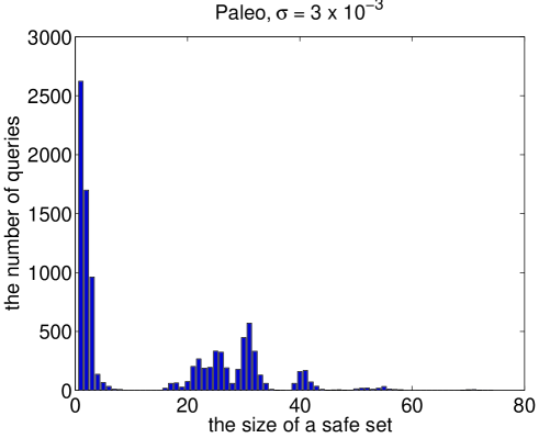
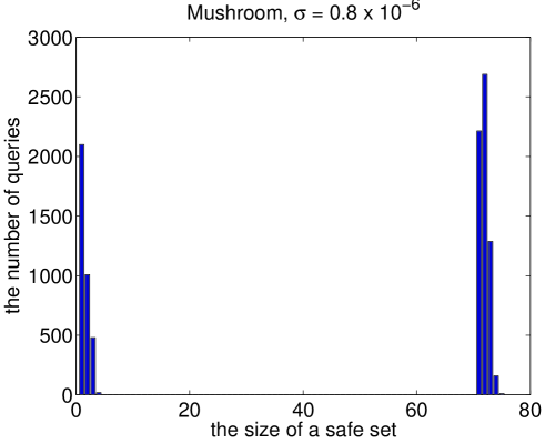
We performed empirical tests to assess the practical relevance of the restricted safe sets, comparing it to the (possibly) unsafe trivial projection. We mined itemset families from two data sets, and estimated boolean queries using both the safe projection and the trivial projection. The first data set, which we call Paleo¹¹1Paleo was constructed from NOW public release 030717 available from [8]., describes fossil findings: the attributes correspond to genera of mammals, the transactions to excavation sites. The Paleo data is sparse, and the genera and sites exhibit strong correlations. The second data set, which we call Mushroom, was obtained from the FIMI repository²²2http://fimi.cs.helsinki.fi. The data is relatively dense.

First we used the Apriori [2] algorithm to retrieve some families of itemsets. A problem with Apriori was that the obtained itemsets were concentrated on the attributes having high frequency. A random query conducted on such a family will be safe with high probability — such a query is trivial to solve. More interesting families would the ones having almost all variables interacting with each other, that is, their dependency graphs have only a small number of isolated nodes. Hence we modified APriori: Let $A$ be the set containing all items and for each $a\in A$ let $m(a)$ be the frequency of $a$. Let $m$ be the smallest frequency $m=\min_{a\in A}m(a)$ and define $s(a)=m(a)/m$. Let $U$ be an itemset and let $\theta_{U}$ be its frequency. Define $\eta_{U}=\prod_{a\in U}s(a)$. We modify Apriori such that the itemset $U$ is in the output if and only if the ratio $\theta_{U}/\eta_{U}$ is larger than given threshold $\sigma$. Note that this family is antimonotonic and so Apriori can be used. By this modification we are trying to give sparse items a fair chance and in our tests the relative frequencies did produce more scattered families.

For each family of itemsets we evaluated $10000$ random boolean queries. We varied the size of the queries between $2$ and $4$. At first, such queries seem too simple but our initial experiments showed that these queries do result large safe sets. A few examples are given in Figure 3. In most of the queries the trivial projection is safe but there are also very large safe sets. Needless to say that we are forced to use restricted safe sets.

Given a query $f$ we calculated two intervals $i_{1}(f)=\operatorname{fi}\left(f\mid\mathcal{F}_{B},\theta_{B}\right)$ and $i_{2}(f)=\operatorname{fi}\left(f\mid\mathcal{F}_{C},\theta_{C}\right)$ where $B$ contains the attributes of $f$ and $C$ is the restricted safe set obtained from $B$ using Algorithm 2. In other words, $i_{1}(f)$ is obtained by using the trivial projection and $i_{2}(f)$ is obtained by projecting to the restricted safe set. As parameters for Algorithm 2 we set the upper bound $M=8$ and the weight function $w$ to be the mutual information.

We divided queries into two classes. A class Trivial contained the queries in which the trivial projection and the restricted safe set were equal. The rest of the queries were labelled as Complex. We also defined a class All that contained all the queries.

As a measure of goodness for a frequency interval we considered the difference between the upper and the lower bound. Clearly $i_{2}(f)\subseteq i_{1}(f)$, so if we define a ratio $r(f)=\frac{\left\|i_{2}(f)\right\|}{\left\|i_{1}(f)\right\|}$, then it is always guaranteed that $0\leq r(f)\leq 1$. Note that the ratio for the queries in Trivial is always $1$.

The ratios were divided into appropriate bins. The results obtained from Paleo data are shown in the contingency table given in Tables 1 and 2 and the results for Mushroom data are given in Tables 3 and 4.

By examining Tables 1 and 2 we conclude the following: If we conduct a random query of form $f$, then in $97\%-99\%$ of the cases the frequency intervals are equal $i_{1}(f)=i_{2}(f)$. However, if we limit ourselves to the cases where the projections differ (the class Complex), then the frequency interval is equal only in about $90\%$ of the cases. In addition, the probability of $i_{1}(f)$ being equal to $i_{2}(f)$ increases as the threshold $\sigma$ grows.

The same observations apply to the results for Mushroom data (Tables 3 and 4): In $93\%-94\%$ of the cases the frequency intervals are equal $i_{1}(f)=i_{2}(f)$, but if we consider only the cases where projections differ, then the percentage drops to $88\%$. The percentages are slightly smaller than those obtained from Paleo data and also there are relatively many queries whose ratios are very small.

The computational burden of a trivial query is equivalent for both trivial projection and restricted safe set. Hence, we examine complex queries in which there is an actual difference in the computational burden. The results suggest that in abt. $10\%$ of the complex queries the restricted safe sets produced tighter interval.

We started our study by considering the following problem: Given a family $\mathcal{F}$ of itemsets, frequencies for $\mathcal{F}$, and a boolean formula find the bounds of the frequency of the formula. This can be solved by linear programming but the problem is that the program has an exponential number of variables. This can be remedied by neglecting the variables not occurring in the boolean formula and thus reducing the dimension. The downside is that the solution may change.

In the paper we defined a concept of safeness: Given an antimonotonic family $\mathcal{F}$ of itemsets a set $C$ of attributes is safe if the projection to $C$ does not change the solution of a query regardless of the query function and the given frequencies for $\mathcal{F}$. We characterised this concept by using graph theory. We also provided an efficient algorithm for finding the minimal safe set containing some given set.

We should point out that while our examples and experiments were focused on conjunctive queries, our theorems work with a query function of any shape

If the family of itemsets satisfies certain requirements, that is, it is triangulated and clique-safe, then we can obtain safe sets from junction trees. We also show that the factorisation obtained from a junction tree can be used to reduce the computational burden of the optimisation problem.

In addition, we provided a heuristic algorithm for finding restricted safe sets. The algorithm tries to construct a set of items such that the optimisation problem does not change for some given itemset frequencies.

We ask ourselves: In practice, should we use the safe sets rather than the trivial projections? The advantage is that the (restricted) safe sets always produce outcome at least as good as the trivial approach. The downside is the additional computational burden. Our tests indicate that if a user makes a random query then in abt. $93\%-99\%$ of the cases the bounds are equal in both approaches. However, this comparison is unfair because there is a large number of queries where the projection sets are equal. To get the better picture we divide the queries into two classes Trivial and Complex, the first containing the queries such that the projections sets are equal, and the second containing the remaining queries. In the first class there is no improvement in the outcome but there is no additional computational burden (checking that the set is safe is cheap comparing to the linear programming). If a query was in Complex, then in $10\%$ of the cases projecting on restricted safe sets did produce more tight bounds.