Salsa Fresca: Angular Embeddings and Pre-Training
for ML Attacks on Learning With Errors

The attack assumes that $t=4n$ initial LWE samples ($\mathbf{a},b$) (rows of ($\mathbf{A,b}$)) with the same secret are available. Sampling $m\leq n$ of the $4n$ initial samples without replacement, $m\times n$ matrices $\mathbf{A}$ and associated $m$-dimensional vectors $\mathbf{b}$ are constructed.

The preprocessing step strives to reduce the norm of the rows of $\mathbf{A}$ by applying a carefully selected integer linear operator $\mathbf{R}$. Because $\mathbf{R}$ is linear with integer entries, the transformed pairs $(\bf RA,Rb)\mod q$ are also LWE pairs with the same secret, albeit larger error. In practice, $\bf R$ is found by performing lattice reduction on the $(m+n)\times(m+n)$ matrix $\mathbf{\Lambda}=\begin{bmatrix}0&q\cdot\mathbf{I}_{n}\\ \omega\cdot\mathbf{I}_{m}&\mathbf{A}\end{bmatrix}$, and finding linear operators $\begin{bmatrix}\mathbf{C}&\mathbf{R}\end{bmatrix}$ such that the norms of $\begin{bmatrix}\mathbf{C}&\mathbf{R}\end{bmatrix}\mathbf{\Lambda}=\begin{bmatrix}\omega\cdot\mathbf{R}&\mathbf{R}\mathbf{A}+q\cdot\mathbf{C}\end{bmatrix}$ are small. This achieves a reduction of the norms of the entries of $\mathbf{RA}\mod q$, but also increases the error in the calculation of ${\bf Rb}={\bf RA\cdot s}+{\bf Re}$, making secret recovery more difficult. Although ML models can learn from noisy data, too much noise will make the distribution of $\bf Rb$ uniform on $[0,q)$ and inhibit learning. The parameter $\omega$ controls the trade-off between norm reduction and error increase. Reduction strength is measured by $\rho=\frac{\sigma(\mathbf{RA})}{\sigma(\mathbf{A})}$, where $\sigma$ denotes the mean of the standard deviations of the rows of $\mathbf{RA}$ and $\mathbf{A}$.

Li et al. (2023a) use BKZ (Schnorr, 1987) for lattice reduction. Li et al. (2023b) improves the reduction time by $45\times$ via a modified definition of the $\Lambda$ matrix and by interleaving BKZ2.0 (Chen & Nguyen, 2011) and polish (Charton et al., 2024) (see Appendix C).

This preprocessing step produces many ($\mathbf{RA},\mathbf{Rb}$) pairs that can be used to train models. Individual rows of $\bf{RA}$ and associated elements of $\mathbf{Rb}$, denoted as reduced LWE samples ($\mathbf{Ra},\mathbf{R}b$) with some abuse of notation, are used for model training. Both the subsampling of $m$ samples from the original $t$ LWE samples and the reduction step are done repeatedly and in parallel to produce 4 million reduced LWE samples, providing the data needed to train the model.

With $4$ million reduced LWE samples ($\mathbf{Ra,R}b$), a transformer is trained to predict $\mathbf{R}b$ from $\mathbf{Ra}$. For simplicity, and without loss of generality, we will say the transformer learns to predict $b$ from $\mathbf{a}$. Li et al. train encoder-decoder transformers (Vaswani et al., 2017) with shared layers (Dehghani et al., 2019). Inputs and outputs consist of integers that are split into two tokens per integer by representing them in a large base $B=\frac{q}{k}$ with $k\approx 10$ and binning the lower digit to keep the vocabulary small as $q$ increases. Training is supervised and minimizes a cross-entropy loss.

The key intuition behind ML-attacks on LWE is that to predict $b$ from $\mathbf{a}$, the model must have learned the secret $\mathbf{s}$. We extract the secret from the model by comparing model predictions for two vectors $\mathbf{a}$ and $\mathbf{a}^{\prime}$ which only differ on one entry. We expect the difference between the model’s predictions for $b$ and $b^{\prime}$ to be small (of the same magnitude as the error) if the corresponding bit of $\mathbf{s}$ is zero, and large if it is non-zero. Repeating the process on all $n$ positions yields a guess for the secret.

For ternary secrets, Li et al. (2023b) introduce a two-bit distinguisher, which leverages the fact that if secret bits $s_{i}$ and $s_{j}$ have the same value, adding a constant $K$ to inputs at both these indices should induce similar predictions. Thus, if $\mathbf{u}_{i}$ is the $i^{th}$ basis vector and $K$ is a random integer, we expect model predictions for $\mathbf{a}+K\mathbf{u}_{i}$ and $\mathbf{a}+K\mathbf{u}_{j}$ to be the same if $s_{i}=s_{j}$. After using this pairwise method to determine whether the non-zero secret bits have the same value, Li et al. classify them into two groups. With only two ways to assign $1$ and $-1$ to the groups of non-zero secret bits, this produces two secret guesses.

Wenger et al. (2022) tests a secret guess $\mathbf{s}^{*}$ by computing the residuals $b-\mathbf{a}\cdot\mathbf{s}^{*}$ over the $4n$ initial LWE sample. If $\mathbf{s}^{*}$ is correct, the standard deviation of the residuals will be close to $\approx\sigma_{e}$. Otherwise, it will be close to the standard deviation of a uniform distribution over $\mathbb{Z}_{q}$: $q/\sqrt{12}$.

For a given dimension, modulus and secret Hamming weight, the performance of ML attacks vary from one secret to the next. Li et al. (2023b) observes that the difficulty of recovering a given secret $\mathbf{s}$ from a set of reduced LWE samples ($\mathbf{a},b$) depends on the distribution of the scalar products $\mathbf{a}\cdot\mathbf{s}$. If a large proportion of these products remain in the interval $(-q/2,q/2)$ (assuming centering) even without a modulo operation, the problem is similar enough to linear regression that the ML attack will usually recover the secret. Li et al. introduce the statistic NoMod: the proportion of scalar products in the training set having this property. They demonstrate that large NoMod strongly correlates with likely secret recoveries for the ML-attack.

Li et al. (2023b) recover binary and ternary secrets, for $n=512$ and $\log_{2}q=41$ LWE problems with Hamming weight $\leq 63$, in about $36$ days, using 4,000 CPUs and one GPU (see their Table 1). Most of the computing resources are needed in the preprocessing stage: reducing one $m\times n$ $\mathbf{A}$ matrix takes about $35$ days, and $4000$ matrices must be reduced to build a training set of $4$ million examples. This suggests two directions for improving the attack performance. First, by introducing fast alternatives to BKZ2.0, we could shorten the time required to reduce one matrix. Second, we could minimize the number of samples needed to train the models, which would reduce the number of CPUs needed for the preprocessing stage.

Another crucial goal is scaling to larger dimensions $n$. The smallest standardized dimension for LWE in the HE Standard (Albrecht et al., 2021) is $n=1024$. At present, ML attacks are limited by their preprocessing time and the length of the input sequences they use. The attention mechanisms used in transformers is quadratic in the length of the sequence, and Li et al. (2023b) encodes $n$ dimensional inputs with $2n$ tokens. More efficient encoding would cut down on transformer processing speed and memory consumption quadratically.

Before presenting our innovations and results, we briefly discuss the LWE settings considered in our work. LWE problems are parameterized by the modulus $q$, the secret dimension $n$, the secret distribution $\chi_{\bf s}$ (sparse binary/ternary) and the hamming weight $h$ of the secret (the number of non-zero entries). Table 3 specifies the LWE problem settings we attack. Proposals for LWE parameter settings in homomorphic encryption suggest using $n=1024$ with sparse secrets (as low as $h=64$), albeit with smaller $q$ than we consider (Curtis & Player, 2019; Albrecht, 2017). Thus, it is important to show that ML attacks can work in practice for dimension $n=1024$ if we hope to attack sparse secrets in real-world settings.

The LWE error distribution remains the same throughout our work: rounded Gaussian with $\sigma=3$ (following Albrecht et al. (2021)). Table 10 in Appendix B contains all experimental settings, including values for the moduli $q$, preprocessing settings, and model training settings.

Encoder-decoder models were originally introduced for machine translation, because their outputs can be longer than their inputs. However, they are complex and slow at inference, because the decoder must run once for each output token. For LWE, outputs (one integer) are always shorter than inputs (a vector of $n$ integers). Li et al. (2023b) observe that an encoder-only model, a 4-layer bidirectional transformer based on DeBERTa (He et al., 2020), achieves comparable performance with their encoder-decoder model.

Here, we experiment with simpler encoder-only models without DeBERTa’s disentangled attention mechanism with $2$ to $8$ layers. Their outputs are max-pooled across the sequence dimension, and decoded by a linear layer for each output digit (Figure 1). We minimize a cross-entropy loss. This simpler architecture improves training speed by $25\%$.

Most transformers process sequences of tokens from a fixed vocabulary, encoded in $\mathbb{R}^{d}$ by a learned embedding. Typical vocabulary sizes vary from $32$K in Llama2 (Touvron et al., 2023), to $256$K in Jurassic-1 (Lieber et al., 2021). The larger the vocabulary, the more data needed to learn the embeddings. LWE inputs and outputs are integers from $\mathbb{Z}_{q}$. For $n\geq 512$ and $q\geq 2^{35}$: encoding integers with one token creates a too-large vocabulary. To avoid this, Li et al. (2023a, b) encode integers with two tokens by representing them in base $B=\frac{q}{k}$ with small $k$ and binning the low digit so the overall vocabulary has $<10$K tokens.

This approach has two limitations. First, input sequences are $2n$ tokens long, which slows training as $n$ grows, because transformers’ attention mechanism scales quadratically in sequence length. Second, all vocabulary tokens are learned independently and the inductive bias of number continuity is lost. Prior work on modular arithmetic (Power et al., 2022; Liu et al., 2022) shows that trained integer embeddings for these problems move towards a circle, e.g. with the embedding of $0$ close to $1$ and $q-1$.

To address these shortcomings, we introduce an angular embedding which strives to better represent the problem’s modular structure in embedding space, while encoding integers with only one token. An integer $a\in\mathbb{Z}_{q}$ is first converted to an angle by the transformation $a\to 2\pi\frac{a}{q}$, and then to the point $(\sin(2\pi\frac{a}{q}),\cos(2\pi\frac{a}{q}))\in\mathbb{R}^{2}$. All input integers (in $\mathbb{Z}_{q}$) are therefore represented as points on the 2-dimensional unit circle, which is then embedded as an ellipse in $\mathbb{R}^{d}$, via a learned linear projection $W_{e}$. Model outputs, obtained by max-pooling the encoder output sequence, are decoded as points in $\mathbb{R}^{2}$ by another linear projection $W_{o}$. The training loss is the $\mathbb{L}_{2}$ distance between the model prediction and the point representing $b$ on the unit circle.

Here, we compare our new architecture with previous work, and assess its performance on larger instances of LWE ($n=768$ and $1024$). All comparisons with prior work are performed on LWE instances with $n=512$ and $\log_{2}q=41$ for binary and ternary secrets, using the same pre-processing techniques as Li et al. (2023b).

To check if angular embedding outperforms vocabulary embedding, we measure the attacked secrets’ NoMod. We expect the better embedding to recover secrets with lower NoMod and higher Hamming weights (e.g. harder secrets). As Figure 2 and Table 6 demonstrate, this is indeed the case. Angular embeddings recover secrets with NoMod$=56$ vs. $63$ for vocabulary embedding (see Table 29 in Appendix F for raw numbers). Furthermore, angular embedding models recover more secrets than those with vocabulary embeddings ($16$ vs. $2$) and succeed on higher $h$ secrets ($66$ vs. $63$). We conclude that an angular embedding is superior to a vocabulary embedding because it recovers harder secrets.

We first consider simply reducing training dataset size and seeing if the attack succeeds. Li et al. always use $4$M training examples. To test if this many is needed for secret recovery, we subsample datasets of size $N$ = [$100$K, $300$K, $1$M, $3$M] from the original $4$M examples preprocessed via the techniques in §3. We train models to attack LWE problems $n=512,\log_{2}q=41$ with binary secrets and $h=30\text{-}45$. Each attack is given 3 days on a single V100 32GB GPU.

Table 9 shows that our attack still succeeds, even when as few as $300$K samples are used. We recover approximately the same number of secrets with $1$M samples as with $4$M, and both settings achieve the same best $h$ recovery. Using $1$M rather than $4$M training samples reduces our preprocessing time by 75%. We run similar experiments for $n=768$ and $n=1024$, and find that we can recover up to $h=13$ secrets for $n=1024$ with only $1$M training samples. Those results are in Tables 18, 18, 20 and 20 in Section E.1.

To further improve sample efficiency, we introduce the first use of pre-training in LWE. Pre-training models has improved sample efficiency in language (Devlin et al., 2019; Brown et al., 2020) and vision (Kolesnikov et al., 2020); we hypothesize similar improvements are likely for LWE. Thus, we frame secret recovery as a downstream task and pre-train a transformer to improve sample efficiency when recovering new secrets, further reducing preprocessing costs.

Formally, an attacker would like to pre-train a model parameterized by $\theta$ on samples $\{(\mathbf{a}^{\prime},b^{\prime})\}$ such that the pre-trained parameters $\theta^{*}$ are a better-than-random initialization for recovering a secret from new samples $\{(\mathbf{a},b)\}$. Although pre-training to get $\theta^{*}$ may require significant compute, $\theta^{*}$ can initialize models for many different secret recoveries, amortizing the initial cost.

The pre-trained weights $\theta^{*}$ should be a good initialization for recovering many different secrets. Thus, we use many different secrets with the 4M rows $\mathbf{Ra}^{\prime}$. In typical recovery, we have 4M rows $\mathbf{Ra}$ and 4M targets $\mathbf{R}b$. In the pre-training setting, however, we generate 150 different secrets so that each $\mathbf{Ra}^{\prime}$ has 150 different possible targets. So the model can distinguish targets, we introduce 150 special vocabulary tokens $t_{s_{i}}$, one for each secret $s_{i}$. We concatenate the appropriate token $t_{s_{i}}$ to row $\mathbf{Ra}^{\prime}$ paired with $\mathbf{R}b^{\prime}=\mathbf{Ra^{\prime}}\cdot\bf s_{i}+e$. Thus, from 4M rows $\mathbf{Ra}^{\prime}$, we produce 600M triplets $(\mathbf{Ra}^{\prime},t_{s_{i}},\mathbf{R}b^{\prime})$. The model learns to predict $\mathbf{R}b^{\prime}$ from a row $\mathbf{Ra}^{\prime}$ and an integer token $t_{s_{i}}$.³³3$t_{s_{i}}$ is embedded using a learned vocabulary.

We hypothesize that including many different $\mathbf{Ra}^{\prime},\mathbf{R}b^{\prime}$ pairs produced from different secrets will induce strong generalization capabilities. When we train the $\theta^{*}$-initialized model on new data with an unseen secret $\bf s$, we indicate that there is a new secret by adding a new token $t_{0}$ to the model vocabulary that serves the same function as $t_{s_{i}}$ above. We randomly initialize the new token embedding, but initialize the remaining model parameters with those of $\theta^{*}$. Then we train and extract secrets as in §2.2.

We use the weights $\theta^{*}$ as the initialization and repeat §5.1’s experiments. We use three different checkpoints from pre-training as $\theta^{*}$ to evaluate the effect of different pre-training amounts: $80$K, $240$K and $440$K pre-training steps.

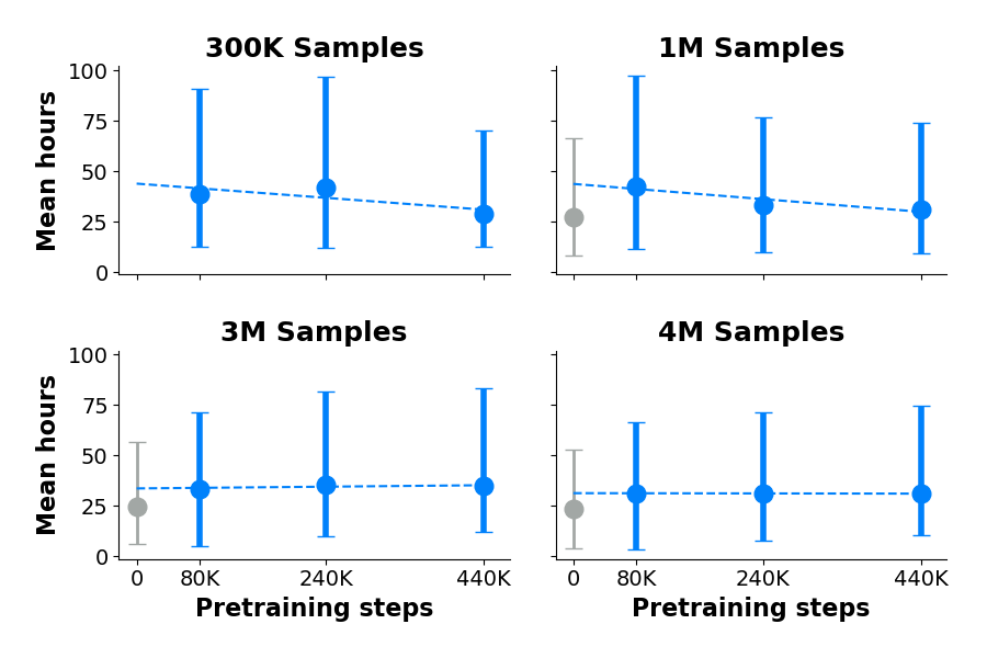
Recall that using fewer samples harms recovery speed (see Table 9). Figure 4 shows trends for recovery speed for pre-trained and randomly initialized models for different numbers of training samples. We find that any pre-training slows down recovery, but further pre-training might minimize this slowdown. Appendix E has complete results.

References

- Ahmadzadeh et al. (2021) Ahmadzadeh, E., Kim, H., Jeong, O., and Moon, I. A Novel Dynamic Attack on Classical Ciphers Using an Attention-Based LSTM Encoder-Decoder Model. IEEE Access, 2021.
- Ajtai (1996) Ajtai, M. Generating hard instances of lattice problems. In Proc. of the ACM symposium on Theory of Computing, 1996.
- Alani (2012) Alani, M. M. Neuro-cryptanalysis of DES and triple-DES. In Proc. of NeurIPS, 2012.
- Albrecht et al. (2021) Albrecht, M., Chase, M., Chen, H., et al. Homomorphic encryption standard. In Protecting Privacy through Homomorphic Encryption, pp. 31–62. 2021. https://eprint.iacr.org/2019/939.
- Albrecht (2017) Albrecht, M. R. On dual lattice attacks against small-secret LWE and parameter choices in HElib and SEAL. In Proc. of EUROCRYPT, 2017. ISBN 978-3-319-56614-6.
- Albrecht et al. (2015) Albrecht, M. R., Player, R., and Scott, S. On the concrete hardness of learning with errors. Journal of Mathematical Cryptology, 9(3):169–203, 2015.
- Albrecht et al. (2017) Albrecht, M. R., Göpfert, F., Virdia, F., and Wunderer, T. Revisiting the expected cost of solving usvp and applications to lwe. In Proc. of ASIACRYPT, 2017.
- Aldarrab & May (2020) Aldarrab, N. and May, J. Can sequence-to-sequence models crack substitution ciphers? arXiv preprint arXiv:2012.15229, 2020.
- Avanzi et al. (2021) Avanzi, R., Bos, J., Ducas, L., Kiltz, E., Lepoint, T., Lyubashevsky, V., Schanck, J. M., Schwabe, P., Seiler, G., and Stehlé, D. CRYSTALS-Kyber (version 3.02) – Submission to round 3 of the NIST post-quantum project. 2021. Available at https://pq-crystals.org/.
- Baek & Kim (2020) Baek, S. and Kim, K. Recent advances of neural attacks against block ciphers. In Proc. of SCIS, 2020.
- Benamira et al. (2021) Benamira, A., Gerault, D., Peyrin, T., and Tan, Q. Q. A deeper look at machine learning-based cryptanalysis. In Proc. of Annual International Conference on the Theory and Applications of Cryptographic Techniques, 2021.
- Brown et al. (2020) Brown, T., Mann, B., Ryder, N., Subbiah, M., Kaplan, J. D., Dhariwal, P., Neelakantan, A., Shyam, P., Sastry, G., Askell, A., et al. Language models are few-shot learners. Proc. of NeurIPS, 2020.
- Charton (2022) Charton, F. Linear algebra with transformers. Transactions in Machine Learning Research, 2022.
- Charton (2024) Charton, F. Can transformers learn the greatest common divisor? arXiv:2308.15594, 2024.
- Charton et al. (2024) Charton, F., Lauter, K., Li, C., and Tygert, M. An efficient algorithm for integer lattice reduction. SIAM Journal on Matrix Analysis and Applications, 45(1), 2024.
- Chen et al. (2020) Chen, H., Chua, L., Lauter, K., and Song, Y. On the Concrete Security of LWE with Small Secret. Cryptology ePrint Archive, Paper 2020/539, 2020. URL https://eprint.iacr.org/2020/539.
- Chen et al. (2022) Chen, L., Moody, D., Liu, Y.-K., et al. PQC Standardization Process: Announcing Four Candidates to be Standardized, Plus Fourth Round Candidates. US Department of Commerce, NIST, 2022. https://csrc.nist.gov/News/2022/pqc-candidates-to-be-standardized-and-round-4.
- Chen & Nguyen (2011) Chen, Y. and Nguyen, P. Q. BKZ 2.0: Better Lattice Security Estimates. In Proc. of ASIACRYPT, 2011.
- Chen & Yu (2021) Chen, Y. and Yu, H. Bridging Machine Learning and Cryptanalysis via EDLCT. Cryptology ePrint Archive, 2021. https://eprint.iacr.org/2021/705.
- Curtis & Player (2019) Curtis, B. R. and Player, R. On the feasibility and impact of standardising sparse-secret LWE parameter sets for homomorphic encryption. In Proc. of the ACM Workshop on Encrypted Computing & Applied Homomorphic Cryptography, 2019.
- Dehghani et al. (2019) Dehghani, M., Gouws, S., Vinyals, O., Uszkoreit, J., and Kaiser, Ł. Universal transformers. In Proc. of ICLR, 2019.
- Devlin et al. (2019) Devlin, J., Chang, M.-W., Lee, K., and Toutanova, K. BERT: Pre-training of deep bidirectional transformers for language understanding. In Proceedings of the Conference of the North American Chapter of the Association for Computational Linguistics, 2019. URL https://aclanthology.org/N19-1423.
- Dubrova et al. (2022) Dubrova, E., Ngo, K., and Gärtner, J. Breaking a fifth-order masked implementation of crystals-kyber by copy-paste. Cryptology ePrint Archive, 2022. https://eprint.iacr.org/2022/1713.
- Dziri et al. (2023) Dziri, N., Lu, X., Sclar, M., Li, X. L., et al. Faith and fate: Limits of transformers on compositionality. arXiv preprint arXiv:2305.18654, 2023.
- Gohr (2019) Gohr, A. Improving attacks on round-reduced speck32/64 using deep learning. In Proc. of Annual International Cryptology Conference, 2019.
- Goncharov (2019) Goncharov, S. V. Using fuzzy bits and neural networks to partially invert few rounds of some cryptographic hash functions. arXiv preprint arXiv:1901.02438, 2019.
- Greydanus (2017) Greydanus, S. Learning the enigma with recurrent neural networks. arXiv preprint arXiv:1708.07576, 2017.
- Griffith & Kalita (2021) Griffith, K. and Kalita, J. Solving Arithmetic Word Problems with Transformers and Preprocessing of Problem Text. arXiv preprint arXiv:2106.00893, 2021.
- Gromov (2023) Gromov, A. Grokking modular arithmetic. arXiv preprint arXiv:2301.02679, 2023.
- He et al. (2020) He, P., Liu, X., Gao, J., and Chen, W. Deberta: Decoding-enhanced bert with disentangled attention. arXiv preprint arXiv:2006.03654, 2020.
- Kaiser & Sutskever (2015) Kaiser, Ł. and Sutskever, I. Neural GPUs learn algorithms. arXiv preprint arXiv:1511.08228, 2015.
- Kalchbrenner et al. (2015) Kalchbrenner, N., Danihelka, I., and Graves, A. Grid long short-term memory. arXiv preprint arxiv:1507.01526, 2015.
- Kimura et al. (2021) Kimura, H., Emura, K., Isobe, T., Ito, R., Ogawa, K., and Ohigashi, T. Output Prediction Attacks on SPN Block Ciphers using Deep Learning. Cryptology ePrint Archive, 2021. URL https://eprint.iacr.org/2021/401.
- Kolesnikov et al. (2020) Kolesnikov, A., Beyer, L., Zhai, X., Puigcerver, J., Yung, J., Gelly, S., and Houlsby, N. Big transfer (bit): General visual representation learning. In Proc. of ECCV, 2020.
- Lample & Charton (2020) Lample, G. and Charton, F. Deep learning for symbolic mathematics. In Proc. of ICLR, 2020.
- Lauter et al. (2011) Lauter, K., Naehrig, M., and Vaikuntanathan, V. Can homomorphic encryption be practical? Proceedings of the 3rd ACM workshop on Cloud computing security workshop, pp. 113–124, 2011.
- Lee et al. (2023) Lee, N., Sreenivasan, K., Lee, J. D., Lee, K., and Papailiopoulos, D. Teaching arithmetic to small transformers. arXiv preprint arXiv:2307.03381, 2023.
- Lenstra et al. (1982) Lenstra, H., Lenstra, A., and Lovász, L. Factoring polynomials with rational coefficients. Mathematische Annalen, 261:515–534, 1982.
- Li et al. (2023a) Li, C. Y., Sotáková, J., Wenger, E., Malhou, M., Garcelon, E., Charton, F., and Lauter, K. Salsa Picante: A Machine Learning Attack on LWE with Binary Secrets. In Proc. of ACM CCS, 2023a.
- Li et al. (2023b) Li, C. Y., Wenger, E., Allen-Zhu, Z., Charton, F., and Lauter, K. E. SALSA VERDE: a machine learning attack on LWE with sparse small secrets. In Proc. of NeurIPS, 2023b.
- Lieber et al. (2021) Lieber, O., Sharir, O., Lenz, B., and Shoham, Y. Jurassic-1: Technical details and evaluation. White Paper. AI21 Labs, 1:9, 2021.
- Liu et al. (2022) Liu, Z., Kitouni, O., Nolte, N. S., Michaud, E., Tegmark, M., and Williams, M. Towards understanding grokking: An effective theory of representation learning. Proc. of NeurIPS, 2022.
- Meng & Rumshisky (2019) Meng, Y. and Rumshisky, A. Solving math word problems with double-decoder transformer. arXiv preprint arXiv:1908.10924, 2019.
- Micciancio & Voulgaris (2010) Micciancio, D. and Voulgaris, P. Faster exponential time algorithms for the shortest vector problem. In Proceedings of the ACM-SIAM Symposium on Discrete Algorithms, 2010.
- Nogueira et al. (2021) Nogueira, R., Jiang, Z., and Lin, J. Investigating the limitations of transformers with simple arithmetic tasks. arXiv preprint arXiv:2102.13019, 2021.
- Palamas (2017) Palamas, T. Investigating the ability of neural networks to learn simple modular arithmetic. 2017. https://project-archive.inf.ed.ac.uk/msc/20172390/msc_proj.pdf.
- Polu & Sutskever (2020) Polu, S. and Sutskever, I. Generative language modeling for automated theorem proving. arXiv preprint arXiv:2009.03393, 2020.
- Power et al. (2022) Power, A., Burda, Y., Edwards, H., Babuschkin, I., and Misra, V. Grokking: Generalization Beyond Overfitting on Small Algorithmic Datasets. arXiv preprint arXiv:2201.02177, 2022.
- Regev (2005) Regev, O. On Lattices, Learning with Errors, Random Linear Codes, and Cryptography. In Proc. of the ACM Symposium on Theory of Computing, 2005.
- Ryan & Heninger (2023) Ryan, K. and Heninger, N. Fast practical lattice reduction through iterated compression. Cryptology ePrint Archive, 2023. URL https://eprint.iacr.org/2023/237.pdf.
- Schnorr (1987) Schnorr, C.-P. A hierarchy of polynomial time lattice basis reduction algorithms. Theoretical Computer Science, 1987. URL https://www.sciencedirect.com/science/article/pii/0304397587900648.
- Siu & Roychowdhury (1992) Siu, K.-Y. and Roychowdhury, V. Optimal depth neural networks for multiplication and related problems. In Proc. of NeurIPS, 1992.
- So (2020) So, J. Deep learning-based cryptanalysis of lightweight block ciphers. Security and Communication Networks, 2020.
- Srivastava & Bhatia (2018) Srivastava, S. and Bhatia, A. On the Learning Capabilities of Recurrent Neural Networks: A Cryptographic Perspective. In Proc. of ICBK, 2018.
- The FPLLL development team (2023) The FPLLL development team. fplll, a lattice reduction library, Version: 5.4.4. Available at https://github.com/fplll/fplll, 2023.
- Touvron et al. (2023) Touvron, H., Martin, L., Stone, K., Albert, P., Almahairi, A., Babaei, Y., et al. Llama 2: Open foundation and fine-tuned chat models. arXiv preprint arXiv:2307.09288, 2023.
- Vaswani et al. (2017) Vaswani, A., Shazeer, N., Parmar, N., et al. Attention is all you need. In Proc. of NeurIPS, 2017.
- Wenger et al. (2022) Wenger, E., Chen, M., Charton, F., and Lauter, K. Salsa: Attacking lattice cryptography with transformers. In Proc. of NeurIPS, 2022.
- Zaremba et al. (2015) Zaremba, W., Mikolov, T., Joulin, A., and Fergus, R. Learning simple algorithms from examples. arXiv preprint arXiv:1511.07275, 2015.
Appendix A Appendix
We provide details, additional experimental results, and analysis ommitted in the main text:
-
1.
Appendix B: Attack parameters
2.
Appendix C: Lattice reduction background
3.
Appendix D: Additional model results (Section 4)
4.
Appendix E: Additional training results (Section 5)
5.
Appendix F: Further NoMod analysis
Appendix B Parameters for our attack
For training all models, we use a learning rate of , weight decay of , 3000 warmup steps, and an embedding dimension of 512. We use encoder layers, and attention heads for all encoder-only model experiments, except the architecture ablation in Table 7. We use the following primes: for , for , and for . The rest of the parameters used for the experiments are in Table 10.