Sampling from Density power divergence-based Generalized posterior distribution
via Stochastic optimization
Abstract
Robust Bayesian inference using density power divergence (DPD) has emerged as a promising approach for handling outliers in statistical estimation. While the DPD-based posterior offers theoretical guarantees for robustness, its practical implementation faces significant computational challenges, particularly for general parametric models with intractable integral terms. These challenges become especially pronounced in high-dimensional settings where traditional numerical integration methods prove inadequate and computationally expensive. We propose a novel sampling methodology that addresses these limitations by integrating the loss-likelihood bootstrap with a stochastic gradient descent algorithm specifically designed for DPD-based estimation. Our approach enables efficient and scalable sampling from DPD-based posteriors for a broad class of parametric models, including those with intractable integrals, and we further extend it to accommodate generalized linear models. Through comprehensive simulation studies, we demonstrate that our method efficiently samples from DPD-based posteriors, offering superior computational scalability compared to conventional methods, particularly in high-dimensional settings. The results also highlight its ability to handle complex parametric models with intractable integral terms.
Keywords: Density power divergence; Generalized Bayes; Bayesian bootstrap; Stochastic optimization
1 Introduction
Bayesian inference is recognized as a powerful statistical methodology across various fields. However, its standard posterior distribution has a notable weakness: sensitivity to outliers that can significantly distort estimation results. To address this challenge, researchers have developed robust alternatives to the standard posterior distribution. A key advancement came from Bissiri et al., (2016), who developed a general framework for updating beliefs through general loss functions in place of the likelihood.
This framework has enabled recent developments in generalized posterior distributions that incorporate robust loss functions to handle outliers effectively. For instance, Ghosh and Basu, (2016) developed a generalized posterior distribution based on the density power divergence (DPD, also known as -divergence) (Basu et al.,, 1998; Eguchi and Kano,, 2001; Minami and Eguchi,, 2002), and proved its theoretical robustness properties. Jewson et al., (2018) further advanced the field by establishing a comprehensive framework for Bayesian inference using general divergence criteria, demonstrating how to achieve robust inference while maintaining Bayesian principles. Additionally, Nakagawa and Hashimoto, (2020) introduced a robust Bayesian estimation method using -divergence (Fujisawa and Eguchi,, 2008), which showed superior performance in variance parameter estimation compared to DPD-based methods. More recently, Matsubara et al., (2022) proposed a robust approach using a Stein discrepancy, which addresses both model misspecification and intractable normalizing constants in likelihood functions.
Within the framework of robust Bayesian inference, the DPD-based posterior, introduced by Ghosh and Basu, (2016), has emerged as a particularly influential approach. While alternative methods such as -divergence may offer stronger theoretical robustness properties, the DPD-based posterior’s theoretical guarantees for robustness against outliers and its well-studied properties across various parametric models make it a natural first choice when considering robust estimation methods. Notably, its robustness properties can be flexibly controlled through a single tuning parameter, enabling practitioners to optimize the trade-off between efficiency and robustness. The selection of this crucial tuning parameter has been extensively studied (Warwick and Jones,, 2005; Basak et al.,, 2021; Yonekura and Sugasawa,, 2023), complementing the method’s theoretical foundations.
Various sampling approaches have been developed for the DPD-based posterior, including Metropolis-Hastings algorithms (Ghosh et al.,, 2022), importance sampling techniques (Ghosh and Basu,, 2016; Nakagawa and Hashimoto,, 2020), and variational Bayesian inference methods (Knoblauch et al.,, 2018). These methodological advances have enabled successful applications across various domains, including online changepoint detection (Knoblauch et al.,, 2018) and differential privacy (Jewson et al.,, 2023).
However, sampling from the DPD-based posterior continues to pose significant computational challenges, particularly for general parametric models. This is primarily due to the presence of intractable integrals or infinite sums in the DPD formulation. Consequently, most studies about the DPD-based posterior have been limited to cases where the normal distribution serves as the probability model.
For general parametric models, while the intractable integral term can theoretically be approximated through numerical integration to enable posterior sampling, this approach often proves inadequate for high-dimensional data (Niederreiter,, 1992). This limitation is particularly problematic given that high-dimensional datasets frequently contain outliers, as demonstrated in the Outlier Detection Datasets (Rayana,, 2016), highlighting the need for robust DPD-based posterior sampling methods that perform well in high-dimensional settings.
A notable step forward in addressing these challenges came from Okuno, (2024), who developed a novel stochastic gradient descent (SGD) algorithm for computing DPD-based estimators. Their approach significantly broadens the applicability of DPD-based estimation to encompass general parametric models, even in cases where the DPD lacks an explicit analytical form. This stochastic methodology offers substantial computational advantages over traditional gradient descent methods using numerical integration, as it eliminates the need for precise integral approximations at each iteration. While their framework provides theoretical convergence guarantees and maintains flexibility in stochastic gradient design, it was primarily developed within a frequentist paradigm.
Building on these developments, we present a novel sampling methodology that bridges the gap between efficient computation and robust Bayesian inference. Our approach leverages the loss-likelihood bootstrap (Lyddon et al.,, 2019) and integrates it with Okuno, (2024)’s SGD algorithm. This integration results in a sampling procedure capable of handling a broad spectrum of parametric models, including those characterized by intractable integrals. We further enhance our methodology by extending it to accommodate generalized linear models, thereby addressing a crucial class of statistical models widely used in practice. Through comprehensive simulation studies, we demonstrate our approach’s computational efficiency, particularly in handling high-dimensional data scenarios.
The remainder of this paper is structured as follows. Section 2 provides a comprehensive overview of generalized Bayesian inference, introducing the theoretical foundations of the DPD-based posterior and the loss-likelihood bootstrap. Section 3 presents our novel methodology, detailing the stochastic gradient-based approach for sampling from DPD-based posteriors and its extension to generalized linear models. Section 4 demonstrates the effectiveness of our proposed method through extensive simulation studies, including validation experiments, comparisons with conventional methods, and applications to intractable models. Finally, Section 5 concludes with a discussion of our findings and future research directions.
2 Generalized Bayesian inference
In this section, we examine the methodological advancements in Bayesian inference under model misspecification and data contamination. We first introduce the generalized posterior distribution, which extends traditional Bayesian methods by incorporating general loss functions and a loss scaling parameter. We then explore the DPD-based posterior as a robust approach for handling outliers, discussing both its theoretical guarantees and computational challenges. Finally, we present the loss-likelihood bootstrap as an efficient method for generating approximate samples from generalized posterior distributions. These foundations will serve as the basis for our proposed novel sampling method in the next section, which specifically addresses the computational challenges in DPD-based posterior inference.
2.1 Generalized Posterior Distribution
Let and denote a sample space and a parameter space, respectively. Suppose that are independent and identically distributed from a distribution , and is a prior probability density function. Let () denote the statistical model on . While Bayesian inference provides methods to quantify uncertainty in , the true data-generating process is often unknown, and the assumed model may be misspecified.
To address this challenge, Bissiri et al., (2016) proposed a general framework for updating belief distributions through what is termed the generalized Bayesian inference. This framework enables quantifying the uncertainty of the general parameter which has the true value , where is a general loss function. The generalized posterior distribution takes the form:
where the loss function has an additive property: (here and throughout, we use the notation to denote ), and is a loss scaling parameter that controls the balance between the prior belief and the information from the data. If we take and , then we get that , which shows that the generalized posterior distribution includes the standard posterior distribution as a special case. The selection of the loss scaling parameter has been extensively studied, as it affects the posterior concentration and the validity of Bayesian inference (Grünwald and van Ommen,, 2017; Holmes and Walker,, 2017; Lyddon et al.,, 2019; Syring and Martin,, 2019; Wu and Martin,, 2023).
To achieve robust Bayesian inference against outliers, we can construct the loss function using robust divergence measures. For example, using DPD or -divergence (Fujisawa and Eguchi,, 2008) instead of the Kullback-Leibler divergence leads to inference procedures that are less sensitive to outliers while maintaining the theoretical guarantees of the generalized Bayesian inference (Ghosh and Basu,, 2016; Nakagawa and Hashimoto,, 2020). These robust divergences provide principled ways to deal with model misspecification and contaminated data while preserving the coherent updating property of Bayesian inference (Jewson et al.,, 2018).
2.2 DPD-based posterior
The DPD offers a particularly attractive approach due to its robustness properties and theoretical guarantees. The DPD-based loss function (Basu et al.,, 1998) is defined for observations as:
| (1) | ||||
| (2) |
where is a tuning parameter and is the distribution corresponding to . The DPD-based posterior (Ghosh and Basu,, 2016) provides a robust framework for updating prior distributions. The DPD-based posterior is defined as:
| (3) | ||||
| (4) |
The DPD-based posterior inherits robust properties from the DPD loss function. Unlike traditional likelihood-based approaches, it is less sensitive to outliers and model misspecification. The robustness of the DPD-based posterior has been theoretically established through the analysis of influence functions (Ghosh and Basu,, 2016). The bounded influence function ensures protection against outliers and model misspecification, while maintaining good efficiency under the true model.
The tuning parameter controls the trade-off between efficiency and robustness, where larger values of provide stronger robustness at the cost of statistical efficiency under correctly specified models. The selection of this parameter in the Bayesian context has been extensively studied (Warwick and Jones,, 2005; Basak et al.,, 2021; Yonekura and Sugasawa,, 2023), providing both theoretical foundations and practical guidelines for choosing appropriate values based on the data characteristics and application context. These studies establish frameworks for parameter selection that maintain the balance between robust inference and computational tractability within the Bayesian paradigm.
The DPD-based posterior has robustness against outliers, which is a highly desirable property. However, the second term of the loss function (2) based on DPD contains an integral term (infinite sum) that cannot be written explicitly, except for specific distributions such as the normal distribution, making it difficult to calculate the posterior distribution using MCMC. While numerical integration can be used to approximate calculations in general probability models, numerical integration often fails for high-dimensional data (Niederreiter,, 1992). To address these computational challenges, we propose a new sampling method that avoids the need for explicit calculation or numerical approximation of the integral term. Before presenting our proposed approach, we first review in the next section the loss-likelihood bootstrap introduced by Lyddon et al., (2019), which will provide important theoretical foundations for our sampling algorithm. The loss-likelihood bootstrap offers a nonparametric way to approximate posterior distributions by resampling, but has limitations when applied directly to DPD-based inference. We will then build on these ideas to develop an efficient sampling scheme specifically designed for DPD posteriors with general parametric models.
2.3 Loss-Likelihood Bootstrap
The loss-likelihood bootstrap (LLB) (Lyddon et al.,, 2019) provides a computationally efficient method for generating approximate samples from generalized posterior distributions by leveraging Bayesian nonparametric principles. The key insight is to model uncertainty about the unknown true data-generating distribution through random weights on the empirical distribution. The algorithm proceeds as follows:
The asymptotic properties of LLB samples are characterized by Theorem 1 (Lyddon et al.,, 2019). This result shows that LLB samples exhibit proper uncertainty quantification asymptotically, with the sandwich covariance matrix providing robustness to model misspecification.
Theorem 1 (Lyddon et al., (2019)).
Let be a proposed LLB sample of a parameter with loss function given observations , and let be its probability measure. Under suitable regularity conditions, for any Borel set , as :
where is the empirical risk minimizer, follows a normal distribution with and , and denotes the gradient operator with respect to .
The LLB approach offers significant computational advantages compared to traditional MCMC methods. By generating independent samples and enabling trivial parallelization, it eliminates the need for convergence diagnostics while maintaining robustness to model misspecification. These properties make it particularly attractive for large-scale inference problems where computational efficiency is crucial.
Moreover, LLB plays a crucial role in calibrating the loss scale parameter for generalized posterior distributions. Under regularity conditions, both the generalized Bayesian posterior and LLB posterior distributions converge to normal distributions with identical means at the empirical risk minimizer but different covariance structures: for the generalized posterior and for the LLB posterior. By equating the Fisher information numbers, defined as for a normal distribution with covariance , they derive the calibration formula . This calibration exhibits a remarkable theoretical property: when the true data-generating distribution belongs to the model family up to a scale factor (i.e., for some and ), it recovers the correct scale . In practice, since is unknown, the matrices and are estimated empirically using the risk minimizer , resulting in a computationally tractable approach for calibrating the generalized posterior that ensures equivalent asymptotic information content with the LLB posterior. This theoretical result, established in (Lyddon et al.,, 2019), provides further justification for viewing LLB as an approximate sampling method from a well-calibrated generalized posterior distribution.
3 Methodology
It is a crucial task for robust Bayesian inference to sample from DPD-based posterior for a general parametric model, but its implementation has been computationally challenging due to the integral terms involved in the DPD calculation. While traditional approaches have been limited to specific probability models where explicit solutions are available, recent advances in stochastic optimization techniques have opened new possibilities for efficient sampling methods. In this section, we propose a novel sampling algorithm that leverages these advances to enable efficient posterior sampling. Our approach reformulates the sampling procedure using stochastic gradient techniques, making it computationally tractable for a broad class of statistical models including GLMs.
3.1 A New Sampling Algorithm from DPD-based posterior
Recently, Okuno, (2024) made a significant breakthrough in minimizing the DPD for general parametric density models by introducing a stochastic optimization approach. While traditional DPD minimization required computing integral terms that could only be explicitly derived for specific distributions such as normal and exponential distributions, their stochastic optimization framework enabled DPD minimization for a much broader class of probability density models.
Inspired by this stochastic approach to minimizing DPD, we propose to reformulate the LLB algorithm (Lyddon et al.,, 2019) as a stochastic method. While LLB was traditionally formulated as an optimization problem based on weighted loss-likelihoods, introducing stochastic optimization techniques enables us to construct a more computationally efficient algorithm.
The objective function, , that we minimize in the LLB algorithm, is
| (5) | |||
| (6) |
We also calculate the gradient of the objective function:
where . Then, we randomly generate independent samples from , and define the stochastic gradient of step by
| (7) |
Taking the expectation of both sides of this equation, we have the following equation:
| (8) | |||
| (9) | |||
| (10) | |||
| (11) |
and confirm that (7) is an unbiased estimator. Let and assume the objective function satisfies the following conditions: (i) is differentiable over (ii) There exists such that for any , (iii) for all (iv) for all . Under these conditions, as , the SGD algorithm converges to minimize the objective function in probability (Ghadimi and Lan,, 2013; Okuno,, 2024). Then, the parameter was iteratively updated by the SGD method:
| (13) |
where is the learning rate satisfying
Based on these theoretical foundations, we implement our approach through the SGD algorithm that offers two key advantages. First, it provides a unified framework that enables sampling from a broad class of parametric probability models, extending beyond the traditional limitations of explicit DPD computations. This generality makes the method applicable across diverse statistical scenarios without requiring model-specific derivations. Second, as demonstrated in subsequent simulation studies, the algorithm exhibits substantial computational efficiency even in high-dimensional settings, where traditional sampling methods often become intractable.
These dual characteristics - theoretical generality and computational tractability - establish our method as a significant contribution to modern statistical inference, particularly in settings requiring both model flexibility and efficient computation. We formalize this approach in Algorithm 2, which details the implementation of our stochastic gradient-based sampling procedure.
3.2 Sampling from DPD-based Posterior in Generalized Linear Models
Building upon the stochastic gradient-based sampling framework introduced in the previous section, we now extend our methodology to encompass generalized linear models (GLMs). As in the previous section, our approach minimizes the objective function through SGD, and all theoretical properties, including the convergence conditions (i)-(iv), remain identical. This theoretical consistency allows us to leverage the same optimization framework while extending its application to the broader class of GLMs.
In GLMs, the random variables are independent and follow the general exponential family of distributions that have density:
| (14) |
where the canonical parameter is a measure of location depending on the fixed predictor and is the scale parameter. Let , so that the GLM satisfies , where is a monotone and differentiable function.
Applying our stochastic gradient-based approach to GLMs, we consider Bayesian inference via DPD for the regression coefficients and the scale parameter. Let and let be a hyperparameter, we can give the following loss function
| (15) | ||||
| (16) |
Following the same principles as our general framework, we derive the stochastic gradient estimator for GLMs. The gradient of the objective function takes the form:
where and is the distribution corresponding to . We randomly generate independent samples from the distribution and . We can acquire the gradient of the objective function such that
| (17) | ||||
| (18) |
Also, is an unbiased estimator from the following calculation.
This generalization advances DPD-based posterior sampling through stochastic gradient methods, particularly addressing models with intractable integral terms in the DPD. Unlike traditional approaches that rely on computationally expensive numerical integration, our method employs stochastic approximation, enabling efficient sampling for various GLMs including Poisson regression. Simulation studies demonstrate that this approach achieves superior computational efficiency and numerical stability while maintaining statistical accuracy. We formalize this method in Algorithm 3, which extends our framework to accommodate GLM-specific characteristics, particularly in gradient computation steps involving multiple samples per observation. The algorithm maintains the core structure of Algorithm 2 while incorporating these GLM-specific modifications.
4 Simulation studies
In this section, we confirm that our proposed method can appropriately sample from the DPD-based posterior. Additionally, we compare our proposed method with conventional approaches to validate its accuracy and efficiency. In all subsequent simulations, the robustness parameter is fixed at .
4.1 Validation of the Proposed Method through Simulations
We evaluated our proposed LLB algorithm, which replaces the objective function’s gradient with an unbiased stochastic gradient, through two comprehensive numerical experiments. For our evaluation dataset, we generated samples from a normal distribution and introduced outliers from at a contamination ratio of . We assumed a normal distribution with parameters as our probability model. This setting is particularly advantageous as it allows us to compute the integral term of (2) explicitly as , enabling us to express the DPD-based posterior in closed form. This tractability facilitates the application of various sampling methods, including MCMC with the Metropolis-Hastings (MH) algorithm and the standard LLB algorithm, providing an ideal framework for comparative analysis.
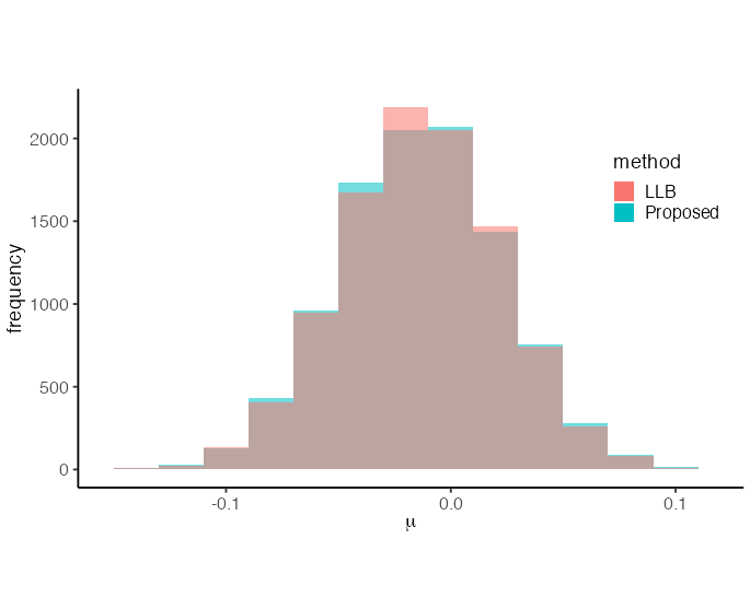
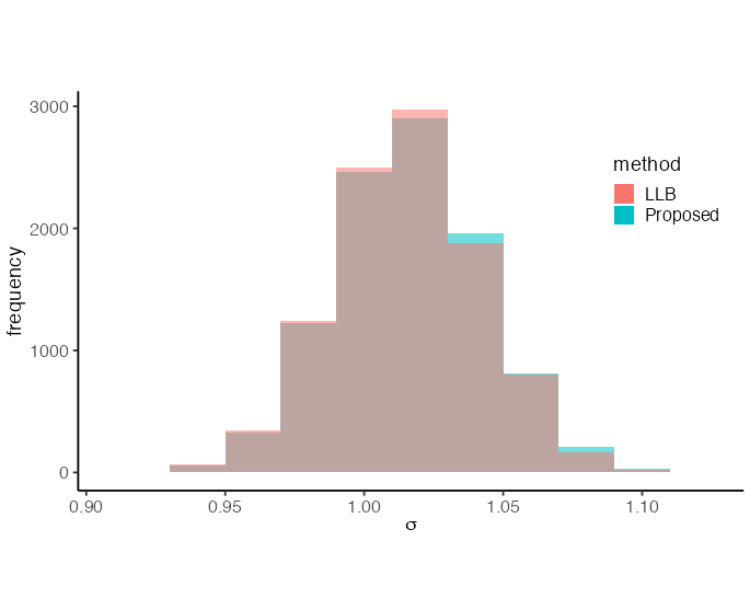
Our first experiment validated that our stochastic gradient approach performs equivalently to the standard LLB algorithm. The results in Figure 1, based on 10000 posterior samples for each method, demonstrate that the performance of the LLB algorithm remains consistent regardless of the stochastic gradient implementation. In our proposed method, we obtained a posterior mean of with posterior variance for and a posterior mean of with posterior variance for . The standard LLB algorithm produced nearly identical results, with posterior mean and posterior variance for , and posterior mean and posterior variance for .
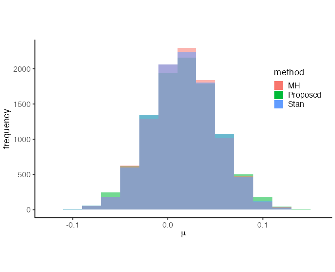
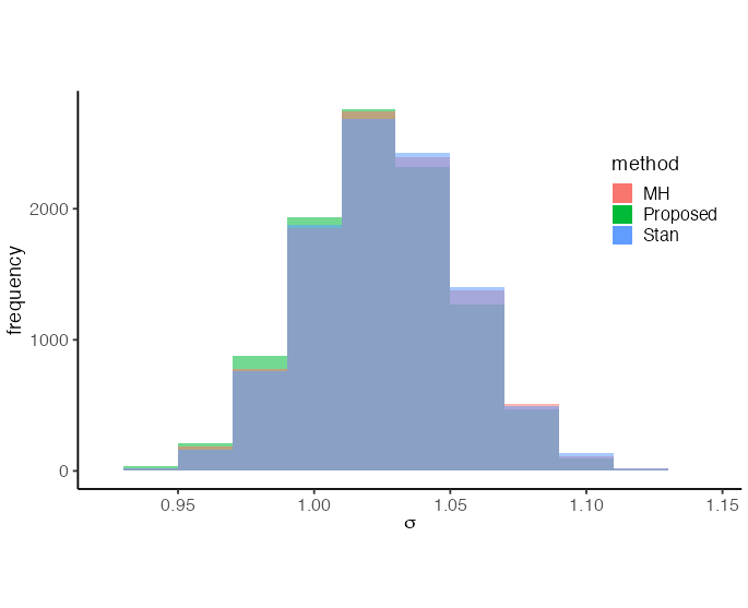
Our second experiment confirmed the accuracy of our proposed method in sampling from the DPD-based posterior. Figure 2 presents overlaid histograms of samples ( samples for each method) obtained from the DPD-based posterior for and using three methods: the MH algorithm, the Hamiltonian Monte Carlo (HMC) method implemented in Stan, and our proposed approach. Our method yielded posterior means of and with posterior variances of and for and , respectively. These results closely aligned with those from the MH algorithm (posterior means of and , posterior variances of and for and ) and the Stan implementation (posterior means of and , posterior variances of and for and ). The close alignment of these distributions empirically validates that our method successfully samples from the target DPD-based posterior.
4.2 Compare with Conventional Algorithms
In high-dimensional settings, conventional sampling methods often face significant computational challenges. These challenges primarily manifest in increased computational time and reduced estimation accuracy. To validate the scalability and effectiveness of our proposed method in addressing these challenges, we conducted a comprehensive simulation study.
To evaluate the validity of our proposed method in high-dimensional settings, we designed our simulation framework using a contaminated multivariate normal model, where we generated samples from with contamination from . Here, denotes the identity matrix and represents a vector of ones. For the numerical integration in the LLB algorithm, we performed the integration over a grid of points spanning the hypercube , where we set grid points per dimension and as the integration boundary. While this grid-based numerical integration approach provides high accuracy for 1-dimensional problems, the computational cost grows exponentially with dimension as it requires evaluations for -dimensional integration. For the optimization in the LLB, we used standard gradient descent with a fixed learning rate . This setting allows us to systematically evaluate the effect of increasing dimensionality. We compared our proposed method against the LLB algorithm with numerical integration, both initialized with maximum likelihood estimates and configured to generate posterior samples.
Table 1 compares the computational efficiency between our SGD approach and the LLB method using gradient descent with numerical integration (GD+NI) across varying dimensions. Through 1000 Monte Carlo simulations, we observed that both methods achieve similar mean squared error values for (SGD: 0.01281, GD+NI: 0.01463) and (SGD: 0.01341, GD+NI: 0.01476), indicating that the estimation accuracy is maintained regardless of the chosen method. The key difference lies in the computational time required to obtain 1000 samples. While SGD maintains consistently low computation times (approximately 3.6-4.0 seconds) regardless of dimension, GD+NI shows an exponential increase in computational cost as the dimension grows. The computational efficiency gain increases exponentially with dimension, reaching a 559-fold improvement at (3.63 seconds for SGD versus 2030.3 seconds for GD+NI). This substantial difference in computational time, while maintaining comparable estimation accuracy, clearly demonstrates the superior scalability of our stochastic approach in higher dimensions.
| Time(Seconds) | ||
|---|---|---|
| SGD | 3.6 | |
| 4.03 | ||
| 3.87 | ||
| 3.63 | ||
| GD+NI | 4.01 | |
| 5.46 | ||
| 134.03 | ||
| 2030.3 |
These empirical results not only support our theoretical findings but also demonstrate the practical viability of our method for high-dimensional robust Bayesian inference. The ability to maintain computational efficiency without sacrificing estimation accuracy makes our method particularly suitable for modern high-dimensional applications where traditional numerical integration approaches become computationally prohibitive.
4.3 Numerical Experiments with Intractable Models
To validate the practical utility of our method in scenarios where traditional approaches face computational challenges, we conducted extensive simulation studies using Poisson regression models. This choice of model is particularly important as it represents a common case where the integral term in (2) lacks a closed-form solution, thus requiring numerical approximation in conventional approaches.
For our simulation setup, we generated synthetic data comprising samples from a Poisson regression model, with the experiment repeated 100 times. The covariates were drawn from a standard multivariate normal distribution , and the response variables were generated according to . The true parameter was constructed by independently sampling each component from a uniform distribution over , ensuring a realistic but challenging estimation scenario.
We compared our proposed stochastic optimization approach against the standard LLB algorithm that relies on finite sum approximation of the infinite sum. For the existing method, we employed the same gradient descent algorithm as described in the previous subsection. Following established practice in the literature (Kawashima and Fujisawa,, 2019), the LLB implementation used Monte Carlo samples for approximation. Both methods were initialized using maximum likelihood estimates and configured to generate posterior samples, ensuring a fair comparison of their performance.
| Performance Measure | Method | ||||
|---|---|---|---|---|---|
| Mean Squared Error | Proposed | 0.0037 | 0.0035 | 0.0037 | 0.0034 |
| Existing | 0.2011 | 0.1353 | 0.0763 | 0.0431 | |
| Coverage Probability | Proposed | 0.923 | 0.943 | 0.941 | 0.954 |
| Existing | 0.797 | 0.708 | 0.739 | 0.812 | |
| Average Length | Proposed | 0.234 | 0.234 | 0.232 | 0.233 |
| Existing | 1.374 | 0.871 | 0.620 | 0.477 |
Table 2 presents a comprehensive comparison across varying dimensions () using three key performance metrics averaged over 100 simulation runs: mean squared error, coverage probability, and average length of 95% credible intervals. To evaluate performance, we first computed the posterior median for each regression coefficient and assessed their accuracy using mean squared error, which is calculated as . Additionally, we constructed 95% credible intervals for each and evaluated their effectiveness using two measures: the average length of the intervals, given by , and the coverage probability, defined as . Our proposed method shows consistently superior performance across all dimensions, not only achieving lower MSE values but also maintaining coverage probabilities closer to the nominal 95% level. Furthermore, it provides more precise uncertainty quantification, as demonstrated by the shorter average interval lengths without compromising coverage.
These results convincingly demonstrate that our stochastic optimization approach delivers more accurate and reliable inference compared to traditional methods, particularly in settings where the model complexity precludes analytical evaluation of the objective function. The robust performance across increasing dimensions further highlights the scalability of our approach, making it particularly attractive for modern high-dimensional applications.
5 Concluding Remarks
This paper introduces a novel stochastic gradient-based methodology for sampling from DPD-based posterior distributions, addressing fundamental challenges in robust Bayesian inference. Our primary contribution lies in developing a computationally efficient approach that overcomes two significant limitations in existing methods: the intractability of integral terms in DPD for general parametric models and the computational burden in high-dimensional settings. The theoretical framework we developed combines the LLB with stochastic gradient descent, providing a robust alternative to traditional MCMC methods while maintaining theoretical guarantees. Through extensive simulation studies, we demonstrated that our method produces samples that accurately represent posterior uncertainty, achieving comparable results to established methods such as MH and HMC algorithms.
A key advantage of our approach is its ability to handle models where the DPD integral term lacks an explicit form, as demonstrated in our application to generalized linear models. The simulation results with Poisson regression highlight not only the method’s computational efficiency but also its superior statistical accuracy compared to conventional approaches. Notably, the method maintains stable estimation performance across varying dimensions, consistently achieving lower mean squared error values and improved coverage probabilities for credible intervals. The practical implications of this work are substantial, offering practitioners a computationally tractable approach to robust Bayesian inference that effectively handles outliers and model misspecification in high-dimensional settings. The method’s success with intractable models, particularly in generalized linear models, suggests broad applicability across diverse statistical applications.
Several promising directions for future research emerge from this work. First, extending the methodology to incorporate informative prior distributions would enable shrinkage estimation, potentially improving parameter estimation in high-dimensional settings where regularization is crucial. Second, adapting the approach to accommodate random effects in generalized linear mixed models would broaden its applicability to hierarchical data structures common in many applied fields. Third, investigating the stability of posterior predictive distributions using our algorithm merits attention, particularly given recent findings by Jewson et al., (2024) regarding the stabilizing effects of DPD-based posteriors on predictive distributions. Additional research directions could include exploring applications to more complex statistical models such as mixture models. Furthermore, establishing theoretical properties under different types of model misspecification and determining optimal choices of the robustness parameter for specific problem settings would enhance the method’s practical utility. In conclusion, our work provides a significant advancement in robust Bayesian computation, offering both theoretical guarantees and practical applicability. The proposed method’s ability to handle high-dimensional and intractable models while maintaining computational efficiency positions it as a valuable tool for modern statistical applications.
References
- Basak et al., (2021) Basak, S., Basu, A., and Jones, M. C. (2021). On the ‘optimal’ density power divergence tuning parameter. Journal of Applied Statistics, 48(3):536–556. PMID: 35706540.
- Basu et al., (1998) Basu, A., Harris, I. R., Hjort, N. L., and Jones, M. (1998). Robust and efficient estimation by minimising a density power divergence. Biometrika, 85(3):549–559.
- Bissiri et al., (2016) Bissiri, P. G., Holmes, C. C., and Walker, S. G. (2016). A general framework for updating belief distributions. Journal of the Royal Statistical Society: Series B (Statistical Methodology), 78(5):1103–1130.
- Eguchi and Kano, (2001) Eguchi, S. and Kano, Y. (2001). Robustifing maximum likelihood estimation by psi-divergence. ISM Research Memorandam, 802:762–763.
- Fujisawa and Eguchi, (2008) Fujisawa, H. and Eguchi, S. (2008). Robust parameter estimation with a small bias against heavy contamination. Journal of Multivariate Analysis, 99(9):2053–2081.
- Ghadimi and Lan, (2013) Ghadimi, S. and Lan, G. (2013). Stochastic first- and zeroth-order methods for nonconvex stochastic programming. SIAM Journal on Optimization, 23(4):2341–2368.
- Ghosh and Basu, (2016) Ghosh, A. and Basu, A. (2016). Robust bayes estimation using the density power divergence. Annals of the Institute of Statistical Mathematics, 68(2):413–437.
- Ghosh et al., (2022) Ghosh, A., Majumder, T., and Basu, A. (2022). General robust bayes pseudo-posteriors: Exponential convergence results with applications. Statistica Sinica, 32(2):pp. 787–823.
- Grünwald and van Ommen, (2017) Grünwald, P. and van Ommen, T. (2017). Inconsistency of Bayesian Inference for Misspecified Linear Models, and a Proposal for Repairing It. Bayesian Analysis, 12(4):1069–1103.
- Holmes and Walker, (2017) Holmes, C. C. and Walker, S. G. (2017). Assigning a value to a power likelihood in a general Bayesian model. Biometrika, 104(2):497–503.
- Jewson et al., (2023) Jewson, J., Ghalebikesabi, S., and Holmes, C. C. (2023). Differentially private statistical inference through -divergence one posterior sampling. In Oh, A., Naumann, T., Globerson, A., Saenko, K., Hardt, M., and Levine, S., editors, Advances in Neural Information Processing Systems, volume 36, pages 76974–77001. Curran Associates, Inc.
- Jewson et al., (2018) Jewson, J., Smith, J. Q., and Holmes, C. (2018). Principles of bayesian inference using general divergence criteria. Entropy, 20(6):442.
- Jewson et al., (2024) Jewson, J., Smith, J. Q., and Holmes, C. (2024). On the Stability of General Bayesian Inference. Bayesian Analysis, pages 1–31.
- Kawashima and Fujisawa, (2019) Kawashima, T. and Fujisawa, H. (2019). Robust and sparse regression in generalized linear model by stochastic optimization. Japanese Journal of Statistics and Data Science, 2(2):465–489.
- Knoblauch et al., (2018) Knoblauch, J., Jewson, J. E., and Damoulas, T. (2018). Doubly robust bayesian inference for non-stationary streaming data with -divergences. In Bengio, S., Wallach, H., Larochelle, H., Grauman, K., Cesa-Bianchi, N., and Garnett, R., editors, Advances in Neural Information Processing Systems, volume 31. Curran Associates, Inc.
- Lyddon et al., (2019) Lyddon, S. P., Holmes, C., and Walker, S. (2019). General bayesian updating and the loss-likelihood bootstrap. Biometrika, 106(2):465–478.
- Matsubara et al., (2022) Matsubara, T., Knoblauch, J., Briol, F.-X., and Oates, C. J. (2022). Robust generalised bayesian inference for intractable likelihoods. Journal of the Royal Statistical Society Series B: Statistical Methodology, 84(3):997–1022.
- Minami and Eguchi, (2002) Minami, M. and Eguchi, S. (2002). Robust blind source separation by beta divergence. Neural computation, 14(8):1859–1886.
- Nakagawa and Hashimoto, (2020) Nakagawa, T. and Hashimoto, S. (2020). Robust bayesian inference via -divergence. Communications in Statistics-Theory and Methods, 49(2):343–360.
- Niederreiter, (1992) Niederreiter, H. (1992). Random Number Generation and Quasi-Monte Carlo Methods. Society for Industrial and Applied Mathematics.
- Okuno, (2024) Okuno, A. (2024). Minimizing robust density power-based divergences for general parametric density models. Annals of the Institute of Statistical Mathematics, pages 1–25.
- Rayana, (2016) Rayana, S. (2016). ODDS library.
- Syring and Martin, (2019) Syring, N. and Martin, R. (2019). Calibrating general posterior credible regions. Biometrika, 106(2):479–486.
- Warwick and Jones, (2005) Warwick, J. and Jones, M. C. (2005). Choosing a robustness tuning parameter. Journal of Statistical Computation and Simulation, 75(7):581–588.
- Wu and Martin, (2023) Wu, P.-S. and Martin, R. (2023). A Comparison of Learning Rate Selection Methods in Generalized Bayesian Inference. Bayesian Analysis, 18(1):105–132.
- Yonekura and Sugasawa, (2023) Yonekura, S. and Sugasawa, S. (2023). Adaptation of the tuning parameter in general bayesian inference with robust divergence. Statistics and Computing, 33(2):39.