Satellite operators with distinct iterates in smooth concordance
Abstract.
Let be a knot in an unknotted solid torus (i.e. a satellite operator or pattern), a knot in and the satellite of with pattern . For any satellite operator , this correspondence gives a function on the set of smooth concordance classes of knots. We give examples of winding number one satellite operators and a class of knots , such that the iterated satellites are distinct as smooth concordance classes, i.e. if , , where each is unknotted when considered as a knot in . This implies that the operators give distinct functions on , providing further evidence for the fractal nature of . There are several other applications of our result, as follows. By using topologically slice knots , we obtain infinite families of topologically slice knots that are distinct in smooth concordance. We can also obtain infinite families of 2–component links (with unknotted components and linking number one) which are not smoothly concordant to the positive Hopf link. For a large class of –space knots (including the positive torus knots), we obtain infinitely many prime knots which have the same Alexander polynomial as but are not themselves –space knots.
2000 Mathematics Subject Classification:
57M251. Introduction
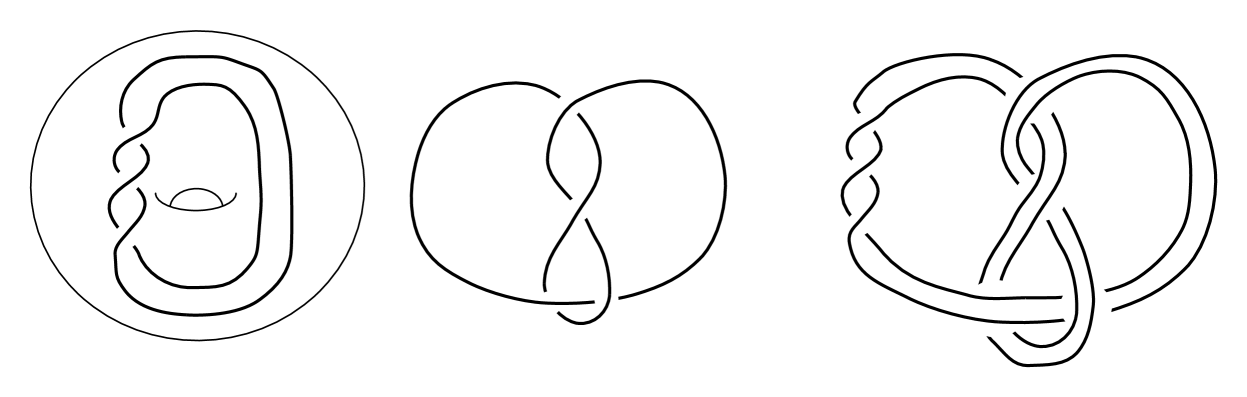
A knot is the image of a smooth embedding . The satellite construction is a well-known function on , the set of isotopy classes of knots. Briefly, a satellite operator is a knot in a solid torus and the satellite knot is obtained by tying the solid torus into the knot . An example of the satellite construction is shown in Figure 1; a more precise definition is given in Section 2.1.
Two knots and are said to be concordant if they cobound a smooth, properly embedded annulus in . modulo concordance forms an abelian group called the knot concordance group, denoted by . Similarly, we say that two knots are exotically concordant if they cobound a smooth, properly embedded annulus in a smooth 4–manifold homeomorphic to (but not necessarily diffeomorphic). modulo exotic concordance forms an abelian group called the exotic knot concordance group, denoted by . If the 4–dimensional smooth Poincaré Conjecture is true, we can see that [CDR14]. The satellite operation on knots descends to well-defined functions on and .
Satellite knots are interesting both within and without knot theory. Satellite operations can be used to construct distinct knot concordance classes which are hard to distinguish using classical invariants, such as in [CHL11, COT04]. In [CFHH13], winding number one satellite operators are used to construct non-concordant knots with homology cobordant zero–surgery manifolds. Satellite operations were used in [Har08] to subtly modify a 3–manifold without affecting its homology type. Winding number one satellite operators in particular are related to Mazur 4–manifolds [AK79] and Akbulut corks [Akb91].
There has been considerable interest in understanding the action of satellite operators on . For instance, it is a famous conjecture that the Whitehead double of a knot is smoothly slice if and only if is smoothly slice [Kir97, Problem 1.38]. This question might be generalized to ask if operators are injective, that is, given an operator , does imply in smooth concordance? A survey of some recent work on the Whitehead doubling operator may be found in [HK12]. In [CHL11], several ‘robust doubling operators’ were introduced and evidence was provided for their injectivity. Not much else is known in the winding number zero case. For operators with nonzero winding numbers, there has been more success. Recently Cochran, Davis and the author proved the following result.
Theorem 1 (Theorem 5.1 of [CDR14]).
If is a strong winding number one satellite operator, the induced function is injective, i.e. for any two knots and , if and only if in . If the 4–dimensional smooth Poincaré Conjecture is true, is injective.
The notion of a ‘strong winding number one’ satellite operator is described in Section 2.1. In particular, any winding number one operator which is unknotted as a knot in is strong winding number one; see Figure 2 for an example.

Theorem 1 is related to the possibility of having a fractal structure. This was conjectured in [CHL11] where some evidence was provided to support this theory. One may characterize ‘fractalness’ of a set as the existence of self-similarities at arbitrarily small scales. By Theorem 1, any strong winding number one satellite operator gives a self-similarity for ; however, while there exist several such operators (see [CDR14, Section 2]), the question of scale has not been addressed. This is the objective of the main theorem of this paper, which follows.
Main Theorem.
For any strong winding number one satellite operator with a Legendrian diagram where and , (e.g. the one shown in Figure 2) and any knot with , the knots are distinct in and . That is, for all in and .
In particular, for the pattern in Figure 2 and knots as above,
Examples of knots with the property that are plentiful. Any knot which is the closure of a positive braid (such as the positive torus knots) has this property. If a knot satisfies this condition, so does its untwisted Whitehead double [Rud95]. In addition, this property is preserved under connected sum of knots. Such knots have the additional property that (this is easily seen using the slice–Bennequin inequality—see Proposition 2.2).
In addition to the operator shown in Figure 2, the main theorem applies to several other satellite operators. Two infinite families of such patterns are given in Figures 9 and 10; see Proposition 3.5 for exact calculations of various invariants for these families.
The action on by the operators in the main theorem should be compared to shrinking the Cantor ternary set by a factor of three, namely that each iteration gives a distinct image of at smaller and smaller scales. To complete the fractal analogy one must also address the question of surjectivity of strong winding number one operators; some progress towards this end has been achieved by Davis and the author in [DR13].
The question of whether the iterates of a satellite operator are distinct is an interesting question in its own right. In particular, there is no known counterpart of our main theorem for the Whitehead doubling operator. It was recently shown in [Par14] that for the torus knots with , and are independent in ; however, we are still unable to distinguish any of the other iterated Whitehead doubles of any knots.
1.1. Applications of the main theorem
Recall that given any knot with , the untwisted Whitehead double of has the same property. Therefore, since any untwisted Whitehead double is topologically slice, we have several examples of topologically slice knots that we may use in our main theorem. For any of the operators as in the main theorem, each will be topologically slice (since is unknotted as a knot in ) and for all in smooth (as well as exotic) concordance. This gives us the following corollary.
Corollary 1.
There exist infinite families of smooth (and exotic) concordance classes of topologically slice knots, where given any two knots in a family, one is a satellite of the other.
Several examples of infinite families of smooth concordance classes of topologically slice knots exist in the literature, such as in [End95, Gom86, HK12, Hom11]. Our examples are novel only due to the ease with which they are obtained and the added property that they are iterated satellites.
We can also obtain an interesting corollary about –space knots, which are defined as follows. A homology sphere is an –space if is the same as that of a lens space (here is the Heegaard–Floer invariant introduced in [OS04]). A knot is called an –space knot if some positive integer surgery on along yields an –space. All positive torus knots, i.e. the knots with , are well-known –space knots, since surgery on them yield lens spaces. –space knots have received much interest lately since their knot Floer complexes may be computed directly from their Alexander polynomials [OS05]. It was also shown in [OS05] that there are strong restrictions on the Alexander polynomial of –space knots. Since several –space knots, we obtain the following corollary.
Corollary 2.
For any –space knot with , there exist infinitely many prime knots with the same Alexander polynomial as which are not themselves –space knots.
As a third application of the main theorem, we can construct infinitely many links which are not smoothly concordant to the Hopf link. Any 2–component link with unknotted gives a satellite operator by considering the knot in the solid torus , where is a regular neighborhood of . It is easy to see that if two such links are concordant they give identical functions on [CDR14, Proposition 2.3]. Given a satellite operator , we may consider the associated 2–component link where is the meridian of the solid torus containing .
Corollary 3.
For any operator in the main theorem, the associated links yield distinct concordance classes of links with linking number one and unknotted components, which are each distinct from the class of the positive Hopf link.
In addition, we know from [CFHH13, Corollary 2.2] that if a winding number one satellite operator is unknotted (such as the one in Figure 2), then the zero–surgery manifolds on and are homology cobordant, for any knot . Recall that the –solvable, positive, negative, and bipolar filtrations of (from [COT04] and [CHH13], denoted by , , , and respectively) can be defined in terms of the zero–surgery manifolds of knots. Therefore, if we start with a knot in (resp. or ) with and an unknotted operator for which the main theorem applies, we obtain a family of infinitely many classes of knots also in (resp. or ). Since if has it has , we cannot directly use the same construction for , but the mirror images of the examples for suffice.
1.2. Acknowledgements
The author would like to thank Tim Cochran, Jung Hwan Park, and Christopher Davis for their time and insightful discussions. We are also indebted to the participants of the Heegaard Floer “computationar” held at Rice University in Spring 2014, particularly Allison Moore and Eamonn Tweedy, for their insights into –space knots and Heegaard–Floer homology.
2. Background
2.1. Satellite operators
A satellite operator, or pattern, is a knot in the standard unknotted solid torus . The winding number of a satellite operator , denoted by , is the signed count of the number of intersections of with a generic meridional disk of .
The set of satellite operators is a monoid in the following natural way. Given a satellite operator in a solid torus , we see the following curves:
-
•
, the meridian of within ,
-
•
, the longitude of within ,
-
•
, the meridian of , and
-
•
, the longitude of .
Given operators , in solid tori , , we construct the composed pattern as follows. Let be a regular neighborhood of inside . Glue and by identifying and . The resulting 3–manifold is a solid torus. The image of inside this solid torus is the desired operator . An example of this construction is shown in Figure 3.
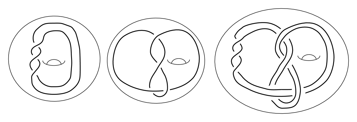
The well-known action of satellite operators on knots is closely related to the above construction. Given a knot and a satellite operator in a solid torus , we obtain the satellite knot as follows. Denote the meridian of by and the longitude by . Let be a tubular neighborhood of . Glue and by identifying and . The resulting 3–manifold is and the image of inside this manifold is the knot . An example of this construction is given in Figure 1. For a survey of the satellite construction see [Lic97, p. 10] or [Rol90, p. 111].
It is easily seen that , i.e. the satellite construction gives a monoid action on . We denote the satellite operator by . Therefore, , i.e. we get the same result whether we start with a knot and apply to it times or we apply the composed pattern to once.
Given a satellite operator , we denote by the knot , where is the unknot. is said to be strong winding number one [CDR14, Definition 1.1] if normally generates . If is unknotted, and are canonically isomorphic and thereofore is strong winding number one if and only if it winding number one [CDR14, Proposition 2.1].
If the knots and are concordant in any 4–manifold bounded by two disjoint copies of , the satellites and are concordant in for every operator . This is easily seen as follows. Let be the concordance between and . We excise a neighborhood of and glue in . The image of in the resulting manifold (which is diffeomorphic to ) is a concordance between and . As a result, the satellite construction is well-defined on and .
2.2. Legendrian knots and the slice–Bennequin inequality
An embedding of a knot in is said to be Legendrian if at each point in it is tangent to the 2–planes of the standard contact structure on . Legendrian knots can be studied concretely through their front projections as in Figure 4. Legendrian knots have two classical invariants, the Thurston–Bennequin number, , and the rotation number, , both of which can be easily calculated via front projections. See [Etn05] for an excellent review of these and related concepts.
Given a Legendrian knot with positive Thurston–Bennequin number, we may repeatedly stabilize at the cost of increasing the rotation number to get a Legendrian diagram with zero Thurston–Bennequin number; such a diagram is a different Legendrian knot, but has the same topological realization as the original knot. See Figure 4 for an example.
We will make use of the slice–Bennequin inequality [Rud95, Rud97][Etn05, pp. 133], which states that for any Legendrian knot ,
Here stands for the smooth 4–genus of a knot, i.e. the least genus of a connected, oriented, smooth, properly embedded surface bounded by in . Since some of our work will be in the exotic category, we show that the slice–Bennequin inequality has an exotic analog.
Definition 2.1.
The exotic 4–genus of a knot , denoted by , is the least genus of a connected, oriented, smooth, properly embedded surface bounded by in a manifold where and is homeomorphic (but not necessarily diffeomorphic) to .
Exotic 4–genus is clearly an invariant of exotic concordance of knots, and is bounded above by the (classical) smooth 4–genus.
Proposition 2.2 (Exotic slice–Bennequin equality).
For a Legendrian knot in
where is Rasmussen’s invariant from Khovanov homology and is Ozsváth–Szabó’s invariant from Heegaard–Floer homology.
2.3. The Legendrian satellite operation
The Legendrian satellite operation is discussed in [Ng01, NT04]. There, a Legendrian pattern in acts on a Legendrian knot in . A front diagram for a Legendrian pattern in shown in Figure 5. In order to construct the (Legendrian) satellite knot we take an –copy of ( ‘vertical’ parallels of ) and insert in a strand of , where is the number of strands of . This process is described in Figure 6. The resulting knot is the –twisted satellite of and . If , the resulting knot is a Legendrian realization of the classical untwisted satellite knot .
The same construction applies when a Legendrian pattern in acts on another pattern also in . This construction is described in Figure 7. The resulting operator is the –twisted –satellite of . Therefore, if , corresponds to the operator described in Section 2.1.
The following lemmata describe how the Thurston–Bennequin number and rotation number of satellites are related.
Lemma 2.3 (Remark 2.4 of [Ng01]).
For a pattern and a knot ,
| (1) |
| (2) |
Lemma 2.4.
For patterns and ,
| (3) |
| (4) |
Proof.
As in Remark 2.4 of [Ng01], these relationships are easily checked using front diagrams of and .∎

3. Proof of the main theorem
For the rest of this section, let denote the pattern shown in Figure 5(b). We easily calculate that , and .
Lemma 3.1.
and .
Proof.
For the rest of this section, fix a non-slice knot with a Legendrian diagram realizing and . There are many examples of such knots, as we mentioned in the introduction. It is easy to see using the (exotic) slice–Bennequin inequality, that such knots have the additional property that .
Proposition 3.2.
for any , even in exotic concordance, where is the operator shown in Figure 2.
Proof.
We can change to by changing a single positive crossing to a negative crossing. Therefore, by Corollary 1.5 of [OS03], we know that
and therefore,
Recall that is an invariant of exotic concordance. Therefore, if even in exotic concordance for some , then . But this implies that for all with , . This contradicts Corollary 3.2 of [CFHH13], which shows exactly that .∎
The following alternate proof uses the technique of the proof of Theorem 3.1 in [CFHH13], which shows that .
Alternate proof of Proposition 3.2.
Using Formulae (1) and (2) and Lemma 3.1 we see that
since . By the exotic slice–Bennequin equality, we have that
Note that and . Therefore,
Therefore, for , even in exotic concordance.
Note that the above process also shows that
and
using the expanded versions of the exotic slice Bennequin inequality given in Proposition 2.2 and since and for any knot .∎
Proposition 3.3.
Given and as above, for any , even in exotic concordance.
Proof.
We can actually make some stronger statements about the operators .
Proposition 3.4.
Given and as above,
for all .
Recall that for the set of knots we are considering. Therefore, this proposition states that
Proof of Proposition 3.4.
The first statement is a consequence of Corollary 1.5 of [OS03] as follows. We saw in the alternate proof of Proposition 3.2 that . Since we can change to by changing a single positive crossing, by Corollary 1.5 of [OS03], we have that
Therefore, . This gives an alternate proof that for .
In the alternate proof of Proposition 3.2, we also saw that . Since and are related by a sequence of crossing changes each of which can be accomplished by adding two bands as shown in Figure 8 we have that, .
Since for any knot , we must have that . Since , we have that . One can construct a Seifert surface for of genus , as pointed out in [CFHH13, Section 3]. For , we can clearly see within the solid torus a genus one surface with two boundary components, one of which is the pattern and the other is the longitude of the solid torus. We glue this surface to a minimal genus Seifert surface for , to see a Seifert surface for with genus . Since , we can proceed by induction. ∎

The techniques in the proof of the main theorem can be easily extended to several other patterns. In particular, consider the families of patterns and shown in Figure 9 and Figure 10 respectively. Note that the pattern is changed to by changing a single positive crossing at the clasp and is the pattern from Figure 2. Similarly, can be changed to by changing a single positive crossing at the top clasp, and is the identity operator (represented by the core of a solid torus).


Proposition 3.5.
For the patterns and and any (shown in Figures 9 and 10) and non-slice knots with Legendrian diagrams realizing and , we have that
For the iterated satellite operators for and , we obtain the following.
We omit the proof of the above proposition since it is virtually identical to the proof of the main theorem. We see that the above statements yield the conditions we obtained in the proof of Proposition 3.4 for , when we set .
We also see easily that our proof works for any satellite operators , which are strong winding number one and have Legendrian realizations realizing and . In short, the proof would consist of using the Alternate proof of Proposition 3.2 to show that , for any and any non-slice knot with a Legendrian diagram realizing . Then, as in the proof of Proposition 3.3, we appeal to Theorem 1, since is strong winding number one.
Together the results of this section constitute the main theorem.
4. Applications
Corollary 1.
We can choose to be topologically slice in the main theorem. This yields an infinite set of topologically slice knots which are distinct in smooth (and exotic) concordance.
Proof.
We can choose to be a topologically slice knot with a Legendrian realization such that , such as the positive untwisted Whitehead double of any knot with this property [Rud95]. If is topologically slice, then is topologically concordant to , which is unknotted. Thereore, for any such , we generate an infinite set of smooth concordance classes of topologically slice knots. ∎
Corollary 2.
For any –space knot with , there exist infinitely many prime knots with the same Alexander polynomial as which are not themselves –space knots.
Proof.
For –space knots which satisfy (such as the positive torus knots), this follows very easily from our main theorem. For the operator , note that since each is unknotted [Sei50, Theorem II]. However, for an –space knot , is equal to the degree of the symmetrized Alexander polynomial. Therefore, since each has the same Alexander polynomial as but have distinct –invariants, they are not –space knots.
In the more general case for an –space knot with , we can still stabilize the Legendrian diagram to get a diagram with and rotation number . Using the same techniques as in the proof of the main theorem, we obtain that
This shows that is unbounded and monotone increasing, and that we can find a subsequence which is strictly increasing and bounded below by , which completes the proof.
If the patterns we use are unknotted as knots in , the knots are prime (see [Cro04, Theorem 4.4.1]). ∎
Corollary 3.
For any operator in the main theorem, the associated links yield distinct concordance classes of links with linking number one and unknotted components, which are each distinct from the class of the positive Hopf link.
Proof.
By Proposition 7.1 of [CDR14], since the functions (as well as , and their iterates) give non-trivial functions on , the corresponding links cannot be smoothly concordant to the positive Hopf link. ∎
References
- [AK79] Selman Akbulut and Robion Kirby. Mazur manifolds. Michigan Math. J., 26(3):259–284, 1979.
- [Akb91] Selman Akbulut. A fake compact contractible -manifold. J. Differential Geom., 33(2):335–356, 1991.
- [CDR14] Tim D. Cochran, Christopher W. Davis, and Arunima Ray. Injectivity of satellite operators in knot concordance. Preprint: http://arxiv.org/abs/1205.5058, To appear: J. Topol., 2014.
- [CFHH13] Tim D. Cochran, Bridget D. Franklin, Matthew Hedden, and Peter D. Horn. Knot concordance and homology cobordism. Proc. Amer. Math. Soc., 141(6):2193–2208, 2013.
- [CHH13] Tim D. Cochran, Shelly Harvey, and Peter Horn. Filtering smooth concordance classes of topologically slice knots. Geom. Topol., 17(4):2103–2162, 2013.
- [CHL11] Tim D. Cochran, Shelly Harvey, and Constance Leidy. Primary decomposition and the fractal nature of knot concordance. Math. Ann., 351(2):443–508, 2011.
- [COT04] Tim D. Cochran, Kent E. Orr, and Peter Teichner. Structure in the classical knot concordance group. Comment. Math. Helv., 79(1):105–123, 2004.
- [Cro04] P.R. Cromwell. Knots and Links. Cambridge University Press, 2004.
- [DR13] Christopher W. Davis and Arunima Ray. Satellite operators as group actions on knot concordance. Preprint: http://arxiv.org/abs/1306.4632, 2013.
- [End95] Hisaaki Endo. Linear independence of topologically slice knots in the smooth cobordism group. Topology Appl., 63(3):257–262, 1995.
- [Etn05] John B. Etnyre. Legendrian and transversal knots. In Handbook of knot theory, pages 105–185. Elsevier B. V., Amsterdam, 2005.
- [Gom86] Robert E. Gompf. Smooth concordance of topologically slice knots. Topology, 25(3):353–373, 1986.
- [Har08] Shelly L. Harvey. Homology cobordism invariants and the Cochran-Orr-Teichner filtration of the link concordance group. Geom. Topol., 12(1):387–430, 2008.
- [HK12] Matthew Hedden and Paul Kirk. Instantons, concordance, and Whitehead doubling. J. Differential Geom., 91(2):281–319, 2012.
- [Hom11] Jennifer Hom. The knot floer complex and the smooth concordance group. Preprint: http://arxiv.org/abs/1111.6635, to appear: Comm. Math. Helv., 2011.
- [Kir97] Rob Kirby, editor. Problems in low-dimensional topology, volume 2 of AMS/IP Stud. Adv. Math. Amer. Math. Soc., Providence, RI, 1997.
- [KM13] P. B. Kronheimer and T. S. Mrowka. Gauge theory and Rasmussen’s invariant. J. Topol., 6(3):659–674, 2013.
- [Lic97] W. B. Raymond Lickorish. An introduction to knot theory, volume 175 of Graduate Texts in Mathematics. Springer-Verlag, New York, 1997.
- [Ng01] Lenhard L. Ng. The Legendrian satellite construction. Preprint: http://arxiv.org/abs/0112105, 2001.
- [NT04] Lenhard L. Ng and Lisa Traynor. Legendrian solid-torus links. J. Symplectic Geom., 2(3):411–443, 2004.
- [OS03] Peter Ozsváth and Zoltán Szabó. Knot Floer homology and the four-ball genus. Geom. Topol., 7:615–639, 2003.
- [OS04] Peter Ozsváth and Zoltán Szabó. Holomorphic disks and topological invariants for closed three-manifolds. Ann. of Math., 3:1027–1158, 2004.
- [OS05] Peter Ozsváth and Zoltán Szabó. On knot Floer homology and lens space surgeries. Topology, 44(6):1281–1300, 2005.
- [Par14] Kyungbae Park. On independence of iterated whitehead doubles in the knot concordance group. Preprint: http://arxiv.org/abs/1311.2050, 2014.
- [Pla04] Olga Plamenevskaya. Bounds for the Thurston-Bennequin number from Floer homology. Algebr. Geom. Topol., 4:399–406, 2004.
- [Rol90] Dale Rolfsen. Knots and links, volume 7 of Mathematics Lecture Series. Publish or Perish Inc., Houston, TX, 1990. Corrected reprint of the 1976 original.
- [Rud95] Lee Rudolph. An obstruction to sliceness via contact geometry and “classical” gauge theory. Invent. Math., 119(1):155–163, 1995.
- [Rud97] Lee Rudolph. The slice genus and the Thurston-Bennequin invariant of a knot. Proc. Amer. Math. Soc., 125(10):3049–3050, 1997.
- [Sei50] H. Seifert. On the homology invariants of knots. Quart. J. Math., Oxford Ser. (2), 1:23–32, 1950.
- [Shu07] Alexander N. Shumakovitch. Rasmussen invariant, slice-Bennequin inequality, and sliceness of knots. J. Knot Theory Ramifications, 16(10):1403–1412, 2007.