Scalable Bayesian Meta-Learning through Generalized Implicit Gradients

Suppose we are given datasets $\mathcal{D}_{t}:=\{(\mathbf{x}_{t}^{n},y_{t}^{n})\}_{n=1}^{N_{t}}$, each of cardinality $|\mathcal{D}_{t}|=N_{t}$ corresponding to a task indexed by $t\in\{1,\ldots,T\}$, where $\mathbf{x}_{t}^{n}$ is an input vector, and $y_{t}^{n}\in\mathbb{R}$ denotes its label. Set $\mathcal{D}_{t}$ is disjointly partitioned into a training set $\mathcal{D}_{t}^{\mathrm{tr}}$ and a validation set $\mathcal{D}_{t}^{\mathrm{val}}$, with $|\mathcal{D}_{t}^{\mathrm{tr}}|=N_{t}^{\mathrm{tr}}$ and $|\mathcal{D}_{t}^{\mathrm{val}}|=N_{t}^{\mathrm{val}}$ for $\forall t$. Typically, $N_{t}$ is limited, and often much smaller than what is required by supervised DL tasks. However, it is worth stressing that the number of tasks $T$ can be considerably large. Thus, $\sum_{t=1}^{T}N_{t}$ can be sufficiently large for learning a prior parameter vector shared by all tasks; e.g., using deep neural networks.

A key attribute of meta-learning is to estimate such a task-invariant prior information parameterized by the meta-parameter $\boldsymbol{\theta}$ based on training data across tasks. Subsequently, $\boldsymbol{\theta}$ and $\mathcal{D}_{t}^{\mathrm{tr}}$ are used to perform task- or inner-level optimization to obtain the task-specific parameter $\boldsymbol{\theta}_{t}\in\mathbb{R}^{d}$. The estimate of $\boldsymbol{\theta}_{t}$ is then evaluated on $\mathcal{D}_{t}^{\mathrm{val}}$ (and potentially also $\mathcal{D}_{t}^{\mathrm{tr}}$) to produce a validation loss. Upon minimizing this loss summed over all the training tasks w.r.t. $\boldsymbol{\theta}$, this meta- or outer-level optimization yields the task-invariant estimate of $\boldsymbol{\theta}$. Note that the dimension of $\boldsymbol{\theta}_{t}$ is not necessarily identical to that of $\boldsymbol{\theta}$; see e.g. (Li et al. 2017; Bertinetto et al. 2019; Lee et al. 2019). As we will see shortly, this nested structure can be formulated as a bi-level optimization problem. This formulation readily suggests application of meta-learning to settings such as hyperparameter tuning that also relies on a similar bi-level optimization (Franceschi et al. 2018).

This bi-level optimization is outlined next for both deterministic and probabilistic Bayesian meta-learning variants.

Delay and memory resources required for solving (2) and (2.1) are arguably the major challenges that meta-learning faces. Here we will elaborate on these challenges in the optimization-based setup, but the same argument carries over to Bayesian meta-learning too.

Consider minimizing the meta-learning loss in (2) using gradient-based iteration such as Adam (Kingma and Ba 2015). In the $(r+1)$-st iteration, gradients must be computed for a batch $\mathcal{B}^{r}\subset\{1,\ldots,T\}$ of tasks. Letting $\hat{\boldsymbol{\theta}}_{t}^{r}:=\hat{\mathcal{A}}_{t}(\hat{\boldsymbol{\theta}}^{r})$, where $\hat{\boldsymbol{\theta}}^{r}$ denotes the meta-parameter in the $r$-th iteration, the chain rule yields the so-termed meta-gradient

where $\nabla\hat{\mathcal{A}}_{t}(\hat{\boldsymbol{\theta}}^{r})$ contains high-order derivatives. When $\hat{\mathcal{A}}_{t}$ is chosen as the one-step GD (cf. (3)), the meta-gradient is

Fortunately, in this case the meta-gradient can still be computed through the Hessian-vector product (HVP), which incurs spatio-temporal complexity $\mathcal{O}(d)$.

In general, $\hat{\mathcal{A}}_{t}$ is a $K$-step GD for some $K>1$, which gives rise to high-order derivatives $\{\nabla^{k}\check{\mathcal{L}}_{t}^{\mathrm{tr}}(\hat{\boldsymbol{\theta}}^{r})\}_{k=2}^{K+1}$ in the meta-gradient. The most efficient computation of the meta-gradient calls for recursive application of HVP $K$ times, what incurs an overall complexity of $\mathcal{O}(Kd)$ in time, and $\mathcal{O}(Kd)$ in space requirements. Empirical wisdom however, favors a large $K$ because it leads to improved accuracy in approximating the true meta-gradient $\nabla_{\boldsymbol{\theta}}\check{\mathcal{L}}_{t}^{\mathrm{val}}(\mathcal{A}_{t}^{*}(\boldsymbol{\theta}))\big{|}_{\boldsymbol{\theta}=\hat{\boldsymbol{\theta}}^{r}}$. Hence, the linear increase of complexity with $K$ will impede the scaling of optimization-based meta-learning algorithms.

When computing the meta-gradient, it should be underscored that the forward implementation of the $K$-step GD function has complexity $\mathcal{O}(Kd)$. However, the constant hidden in the ${\cal O}$ is much smaller compared to the HVP computation in the backward propagation. Typically, the constant is $1/5$ in terms of time and $1/2$ in terms of space; see  (Griewank 1993; Rajeswaran et al. 2019). For this reason, we will focus on more efficient means of obtaining the meta-gradient function $\nabla_{\boldsymbol{\theta}}\mathcal{L}_{t}^{\mathrm{val}}(\hat{\mathcal{A}}_{t}(\boldsymbol{\theta}))$ for Bayesian meta-learning. It is also worth stressing that our results in the next section will hold for an arbitrary vector $\boldsymbol{\theta}\in\mathbb{R}^{d}\times\mathbb{R}_{>0}^{d}$ instead of solely the variable $\hat{\boldsymbol{\theta}}^{r}$ of the $r$-th iteration. Thus, we will use the general vector $\boldsymbol{\theta}$ when introducing our approach, while we will take its value at the point $\boldsymbol{\theta}=\hat{\boldsymbol{\theta}}^{r}$ when presenting our meta-learning algorithm.

We start with decomposing the meta-gradient in Bayesian meta-learning (2.1) (henceforth referred to as Bayesian meta-gradient) using the chain rule

where $\nabla_{1}$ and $\nabla_{2}$ denote the partial derivatives of a function w.r.t. its first and second arguments, respectively. The computational burden in (3.1) comes from the high-order derivatives present in the Jacobian $\nabla\hat{\mathcal{A}}_{t}(\boldsymbol{\theta})$.

The key idea behind implicit differentiation is to express $\nabla\hat{\mathcal{A}}_{t}(\boldsymbol{\theta})$ as a function of itself, so that it can be numerically obtained without using high-order derivatives. The following lemma formalizes how the implicit Jacobian is obtained in our setup. All proofs can be found in the Appendix.

Two remarks are now in order regarding the technical assumption, and connections with iMAML. For notational brevity, define the block matrix

An immediate consequence of Lemma 1 is the so-called generalized implicit gradients. Suppose that $\hat{\mathcal{A}}_{t}$ involves a $K$ sufficiently large for the sub-optimal point $\hat{\mathbf{v}}_{t}$ to be close to a local optimum $\bar{\mathbf{v}}_{t}$. The Bayesian meta-gradient (3.1) can then be approximated through

The approximate implicit gradient in (14) is computationally expensive due to the matrix inversion $\mathbf{H}_{t}^{-1}(\hat{\mathbf{v}}_{t})$, which incurs complexity $\mathcal{O}(d^{3})$. To relieve the computational burden, a key observation is that $\mathbf{H}_{t}^{-1}(\hat{\mathbf{v}}_{t})\nabla_{1}\mathcal{L}_{t}^{\mathrm{val}}(\hat{\mathbf{v}}_{t},\boldsymbol{\theta})$ is the solution of the optimization problem

Given that the square matrix $\mathbf{H}_{t}(\hat{\mathbf{v}}_{t})$ is by definition symmetric, problem (15) can be efficiently solved using the conjugate gradient (CG) iteration. Specifically, the complexity of CG is dominated by the matrix-vector product $\mathbf{H}_{t}(\hat{\mathbf{v}}_{t})\mathbf{p}$ (for some vector $\mathbf{p}\in\mathbb{R}^{2d}$), given by

The first term on the right-hand side of (16) is an HVP, and the second is the multiplication of a diagonal matrix with a vector. Note that with the diagonal matrix, the latter term boils down to a dot product, implying that the complexity of each CG iteration is as low as $\mathcal{O}(d)$. In practice, a small number of CG iterations suffices to produce an accurate estimate of $\mathbf{H}_{t}^{-1}(\hat{\mathbf{v}}_{t})\nabla_{1}\mathcal{L}_{t}^{\mathrm{val}}(\hat{\mathbf{v}}_{t},\boldsymbol{\theta})$ thanks to its fast convergence rate (Van der Sluis and van der Vorst 1986; Winther 1980). In order to control the total complexity of iBaML, we set the maximum number of CG iterations to a constant $L$.

Having obtained an approximation of the matrix-inverse-vector product $\mathbf{H}_{t}^{-1}(\hat{\mathbf{v}}_{t})\nabla_{1}\mathcal{L}_{t}^{\mathrm{val}}(\hat{\mathbf{v}}_{t},\boldsymbol{\theta})$, we proceed to estimate the Bayesian meta-gradient. Let $\hat{\mathbf{u}}_{t}:=[\hat{\mathbf{u}}_{t,\mathbf{m}}^{\top},\hat{\mathbf{u}}_{t,\mathbf{d}}^{\top}]^{\top}$ be the output of the CG method with subvectors $\hat{\mathbf{u}}_{t,\mathbf{m}},~{}\hat{\mathbf{u}}_{t,\mathbf{d}}\in\mathbb{R}^{d}$. Then, it follows from (14) that

where we also used the definition (11). Again, the diagonal-matrix-vector products in (3.1) can be efficiently computed through dot products, which incur complexity $\mathcal{O}(d)$. The step-by-step pseudocode of the iBaML is listed under Algorithm 1.

In a nutshell, the implicit Bayesian meta-gradient computation consumes $\mathcal{O}(Ld)$ time, regardless of the optimization algorithm $\hat{\mathcal{A}}_{t}$. One can even employ more complicated algorithms such as second-order matrix-free optimization (Martens and Grosse 2015; Botev, Ritter, and Barber 2017). In addition, as the time complexity does not depend on $K$, one can increase $K$ to reduce the approximation error in (14). The space complexity of iBaML is only $\mathcal{O}(d)$ thanks to the iterative implementation of CG steps. These considerations explain how iBaML addresses the scalability issue of explicit backpropagation.

This section deals with performance analysis of both explicit and implicit gradients in Bayesian meta-learning to further understand their differences. Similar to (Rajeswaran et al. 2019), our results will rely on the following assumptions.

Based on these assumptions, we can establish the following result.

Theorem 1 asserts that the $\ell_{2}$ error of the explicit Bayesian meta-gradient relative to the true depends on the task-level optimization error as well as the error in the Jacobian, where the former captures the Euclidean distance of the local minimum $\bar{\mathbf{v}}_{t}$ and its approximation $\hat{\mathbf{v}}_{t}$, while the latter characterizes how the sub-optimal function $\hat{\mathcal{A}}_{t}$ influences the Jacobian. Both errors can be reduced by increasing $K$ in the task-level optimization, at the cost of time and space complexity for backpropagating $\nabla\hat{\mathcal{A}}_{t}(\boldsymbol{\theta})$. Ideally, one can have $\delta_{t}=0$ when $\hat{\mathbf{v}}_{t}$ is a local optimum, and $\epsilon_{t}=0$ when choosing $\bar{\mathbf{v}}_{t}=\hat{\mathbf{v}}_{t}$.

Next, we derive an error bound for implicit differentiation.

While the bound on implicit meta-gradient also depends on the task-level optimization error, the difference with Theorem 1 is highlighted in the CG error. The fast convergence of CG leads to a tolerable $\delta_{t}^{\prime}$ even with a small $L$. As a result, one can opt for a large $K$ to reduce task-level optimization error $\epsilon_{t}$, and a small $L$ to obtain a satisfactory approximation of the meta-gradient.

It is worth stressing that $\bar{\mathbf{v}}_{t}$ in Theorems 1 and 2 can denote any local optimum. It further follows by definition that both $\delta_{t}$ and $\delta_{t}^{\prime}$ do not rely on the choice of local optima, yet $\epsilon_{t}$ does. One final remark is now in order.

Here we experiment on the errors between explicit and implicit gradients over a synthetic dataset. The data are generated using the Bayesian linear regression model

where $\{\boldsymbol{\theta}_{t}\}_{t=1}^{T}$ are i.i.d. samples drawn from a distribution $p(\boldsymbol{\theta}_{t};\hat{\boldsymbol{\theta}})$ that is unknown during meta-training, and $e_{t}^{n}$ is the additive white Gaussian noise (AWGN) with known variance $\sigma^{2}$. Although the current training posterior $p(\boldsymbol{\theta}_{t}|y_{t}^{\mathrm{tr}};\mathbf{X}_{t}^{\mathrm{tr}},\boldsymbol{\theta})$ becomes tractable, we still focus on the VI approximation for uniformity. Within this rudimentary linear case, it can be readily verified that the task-level optimum $\mathbf{v}_{t}^{*}:=[\mathbf{m}_{t}^{*\top},\mathbf{d}_{t}^{*\top}]^{\top}$ of (5) is given by

where $\operatorname{diag}(\mathbf{M})$ is a vector collecting the diagonal entries of matrix $\mathbf{M}$. The true posterior in the linear case is $p(\boldsymbol{\theta}_{t}|\mathbf{y}_{t}^{\mathrm{tr}};\mathbf{X}_{t}^{\mathrm{tr}},\boldsymbol{\theta})=\mathcal{N}(\mathbf{m}_{t}^{*},\big{(}\frac{1}{2\sigma^{2}}(\mathbf{X}_{t}^{\mathrm{tr}}(\mathbf{X}_{t}^{\mathrm{tr}})^{\top})+\mathbf{d}^{-1}\big{)}^{-1})$, implying that the posterior covariance matrix is essentially approximated by its diagonal counterpart $\mathbf{D}_{t}^{*}$ in VI. Lemma 1 and (3.1) imply that the oracle meta-gradient is

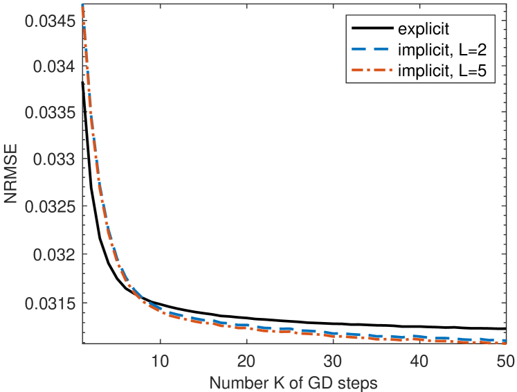
As a benchmark meta-learning algorithm, we selected the amortized Bayesian meta-learning (ABML) in (Ravi and Beatson 2019). The metric used for performance assessment is the normalized root-mean-square error (NRMSE) between the true meta-gradient $\nabla_{\boldsymbol{\theta}}\mathcal{L}_{t}^{\mathrm{val}}(\mathbf{v}_{t}^{*}(\boldsymbol{\theta}),\boldsymbol{\theta})$, and the estimated meta-gradients $\nabla_{\boldsymbol{\theta}}\mathcal{L}_{t}^{\mathrm{val}}(\hat{\mathbf{v}}_{t}(\boldsymbol{\theta}),\boldsymbol{\theta})$ and $\hat{\mathbf{g}}_{t}$; see also the Appendix for additional details on the numerical test.

Figure 1 depicts the NRMSE as a function of $K$ for the first iteration of ABML, that is at the point $\boldsymbol{\theta}=\hat{\boldsymbol{\theta}}^{0}$. For explicit and implicit gradients, the NRMSE decreases as $K$ increases, while the former outperforms the latter for $K\leq 5$, and the vice-versa for $K>5$. These observations confirm our analytical results. Intuitively, factors $F_{t}\epsilon_{t}$ and $F_{t}^{\prime}\epsilon_{t}$ caused by imprecise task-level optimization dominate the upper bounds for small $K$, thus resulting in large NRMSE. Besides, implicit gradients are more sensitive to task-level optimization errors. One conjecture is that iBaML is developed based on Lemma 1, where the matrix inversion can be sensitive to $\bar{\mathbf{v}}_{t}$’s variation. Despite that the conditioning number $\kappa$ of $\mathbf{X}_{t}^{\mathrm{tr}}$ takes on a large value purposely so that $\epsilon_{t}$ decreases slowly with $K$, a small $K$ suffices to capture accurately implicit gradients. The main reason is that the CG error $\delta_{t}^{\prime}$ can become sufficiently small even with only $L=2$ steps, while $\delta_{t}$ remains large because GD converges slowly.

Next, we conduct tests to assess the performance of iBaML on real datasets. We consider one of the most widely used few-shot dataset for classification miniImageNet (Vinyals et al. 2016). This dataset consists of natural images categorized in $100$ classes, with $600$ samples per class. All images are cropped to have size of $84\times 84$. We adopt the dataset splitting suggested by (Ravi and Larochelle 2017), where $64$, $16$ and $20$ disjoint classes are used for meta-training, meta-validation and meta-testing, respectively. The setups of the numerical test follow from the standard $W$-class $S^{\mathrm{tr}}$-shot few-shot learning protocol in (Vinyals et al. 2016). In particular, each task has $W$ randomly selected classes, and each class contains $S^{\mathrm{tr}}$ training images and $S^{\mathrm{val}}$ validation images. In other words, we have $N^{\mathrm{tr}}=S^{\mathrm{tr}}W$ and $N^{\mathrm{val}}=S^{\mathrm{val}}W$. We further adopt the typical choices with $W=5$, $S^{\mathrm{tr}}\in\{1,5\}$, and $S^{\mathrm{val}}=15$. It should be noted that the training and validation sets are also known as support and query sets in the context of few-shot learning.

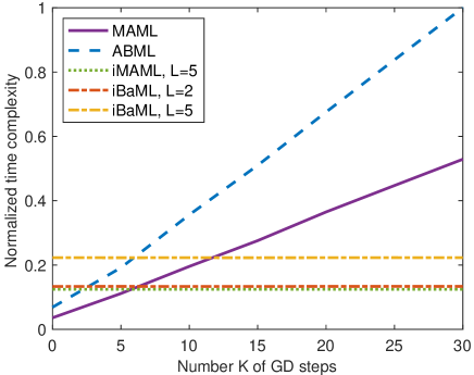
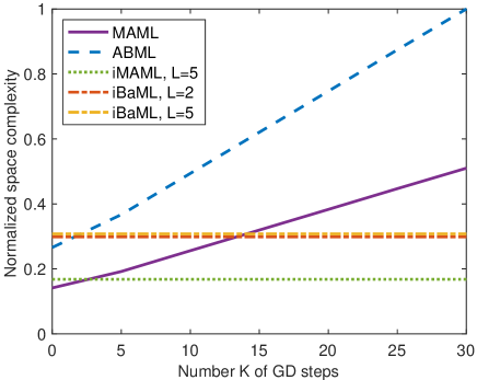
We first empirically compare the computational complexity (time and space) for explicit versus implicit gradients on the $5$-class $1$-shot miniImageNet dataset. Here we are only interested in backward complexity, so the delay and memory requirements for forward pass of $\hat{\mathcal{A}}_{t}$ is excluded. Figure 2(a) plots the time complexity of explicit and implicit gradients against $K$. It is observed that the time complexity of explicit gradient grows linearly with $K$, while the implicit one increases only with $L$ but not $K$. Moreover, the explicit and implicit gradients have comparable time complexity when $K=L$. As far as space complexity, Figure 2(b) illustrates that memory usage with explicit gradients is proportional to $K$. In contrast, the memory used in the implicit gradient algorithms is nearly invariant across $K$ values. Such a memory-saving property is important when meta-learning is employed with models of growing degrees of freedom. Furthermore, one may also notice from both figures that MAML and iMAML incur about $50\%$ time/space complexities of ABML and iBaML. This is because non-Bayesian approaches only optimize the mean vector of the Gaussian prior, whose dimension is $d$, while the probabilistic methods cope with both the mean and diagonal covariance matrix of the pdf with corresponding dimension $2d$. This increase in dimensionality doubles the space-time complexity in gradient computations.

Next, we demonstrate the effectiveness of iBaML in reducing the Bayesian meta-learning loss. The test is conducted on the $5$-class $5$-shot miniImageNet. The model is a standard $4$-layer $32$-channel convolutional neural network, and the chosen baseline algorithms are MAML (Finn, Abbeel, and Levine 2017) and ABML (Ravi and Beatson 2019); see also the Appendix for alternative setups. Due to the large number of training tasks, it is impractical to compute the exact meta-training loss. As an alternative, we adopt the ‘test nll’ (averaged over $1,000$ test tasks) as our metric, and also report their corresponding accuracy. For fairness, we set $L=5$ when implementing the implicit gradients so that the time complexity is similar to explicit one with $K=5$. The results are listed in Table 1. It is observed that both nll and accuracy improve with $K$, implying that the meta-learning loss can be effectively reduced by trading a small error in gradient estimation.

To quantify the uncertainties embedded in state-of-the-art meta-learning methods, Figure 3 plots the expected/maximum calibration errors (ECE/MCE) (Naeini, Cooper, and Hauskrecht 2015). It can be seen that iBaML is once again the most competitive among tested approaches.

References

• Abbas et al. (2022) Abbas, M.; Xiao, Q.; Chen, L.; Chen, P.-Y.; and Chen, T. 2022. Sharp-MAML: Sharpness-Aware Model-Agnostic Meta Learning. In Proceedings of the 39th International Conference on Machine Learning, volume 162 of Proceedings of Machine Learning Research, 10–32. PMLR.
• Bengio, Bengio, and Cloutier (1995) Bengio, S.; Bengio, Y.; and Cloutier, J. 1995. On the Search for New Learning Rules for ANNs. Neural Processing Letters, 2(4): 26–30.
• Bertinetto et al. (2019) Bertinetto, L.; Henriques, J. F.; Torr, P.; and Vedaldi, A. 2019. Meta-learning with Differentiable Closed-Form Solvers. In Proceedings of International Conference on Learning Representations.
• Botev, Ritter, and Barber (2017) Botev, A.; Ritter, H.; and Barber, D. 2017. Practical Gauss-Newton Optimisation for Deep Learning. In Proceedings of the 34th International Conference on Machine Learning, volume 70 of Proceedings of Machine Learning Research, 557–565. PMLR.
• Chen and Chen (2022) Chen, L.; and Chen, T. 2022. Is Bayesian Model-Agnostic Meta Learning Better than Model-Agnostic Meta Learning, Provably? In Proceedings of The 25th International Conference on Artificial Intelligence and Statistics, volume 151 of Proceedings of Machine Learning Research, 1733–1774. PMLR.
• Fallah, Mokhtari, and Ozdaglar (2020) Fallah, A.; Mokhtari, A.; and Ozdaglar, A. 2020. On the Convergence Theory of Gradient-Based Model-Agnostic Meta-Learning Algorithms. In Proceedings of the Twenty Third International Conference on Artificial Intelligence and Statistics, volume 108, 1082–1092. PMLR.
• Finn, Abbeel, and Levine (2017) Finn, C.; Abbeel, P.; and Levine, S. 2017. Model-Agnostic Meta-Learning for Fast Adaptation of Deep Networks. In Proceedings of the 34th International Conference on Machine Learning, volume 70, 1126–1135. PMLR.
• Finn, Xu, and Levine (2018) Finn, C.; Xu, K.; and Levine, S. 2018. Probabilistic Model-Agnostic Meta-Learning. In Advances in Neural Information Processing Systems, volume 31. Curran Associates, Inc.
• Flennerhag et al. (2020) Flennerhag, S.; Rusu, A. A.; Pascanu, R.; Visin, F.; Yin, H.; and Hadsell, R. 2020. Meta-Learning with Warped Gradient Descent. In Proceedings of International Conference on Learning Representations.
• Franceschi et al. (2018) Franceschi, L.; Frasconi, P.; Salzo, S.; Grazzi, R.; and Pontil, M. 2018. Bilevel Programming for Hyperparameter Optimization and Meta-Learning. In Proceedings of the 35th International Conference on Machine Learning, volume 80, 1568–1577. PMLR.
• Grant et al. (2018) Grant, E.; Finn, C.; Levine, S.; Darrell, T.; and Griffiths, T. 2018. Recasting Gradient-Based Meta-Learning as Hierarchical Bayes. In Proceedings of International Conference on Learning Representations.
• Griewank (1993) Griewank, A. 1993. Some bounds on the complexity of gradients, Jacobians, and Hessians. In Complexity in numerical optimization, 128–162. World Scientific.
• Hansen and Wang (2021) Hansen, N.; and Wang, X. 2021. Generalization in Reinforcement Learning by Soft Data Augmentation. In 2021 IEEE International Conference on Robotics and Automation (ICRA), 13611–13617.
• Kingma and Ba (2015) Kingma, D. P.; and Ba, J. 2015. Adam: A Method for Stochastic Optimization. In Proceedings of International Conference on Learning Representations.
• Lee et al. (2019) Lee, K.; Maji, S.; Ravichandran, A.; and Soatto, S. 2019. Meta-Learning With Differentiable Convex Optimization. In Proceedings of the IEEE/CVF Conference on Computer Vision and Pattern Recognition (CVPR).
• Li et al. (2017) Li, Z.; Zhou, F.; Chen, F.; and Li, H. 2017. Meta-sgd: Learning to learn quickly for few-shot learning. arXiv preprint arXiv:1707.09835.
• Martens and Grosse (2015) Martens, J.; and Grosse, R. 2015. Optimizing Neural Networks with Kronecker-factored Approximate Curvature. In Proceedings of the 32nd International Conference on Machine Learning, volume 37 of Proceedings of Machine Learning Research, 2408–2417. Lille, France: PMLR.
• Miao, Metze, and Rawat (2013) Miao, Y.; Metze, F.; and Rawat, S. 2013. Deep maxout networks for low-resource speech recognition. In 2013 IEEE Workshop on Automatic Speech Recognition and Understanding, 398–403. IEEE.
• Mishra et al. (2018) Mishra, N.; Rohaninejad, M.; Chen, X.; and Abbeel, P. 2018. A Simple Neural Attentive Meta-Learner. In International Conference on Learning Representations.
• Naeini, Cooper, and Hauskrecht (2015) Naeini, M. P.; Cooper, G.; and Hauskrecht, M. 2015. Obtaining well calibrated probabilities using bayesian binning. In Proceedings of the Twenty Ninth International Conference on Artificial Intelligence and Statistics, 2901–2907. PMLR.
• Nguyen, Do, and Carneiro (2020) Nguyen, C.; Do, T.-T.; and Carneiro, G. 2020. Uncertainty in Model-Agnostic Meta-Learning using Variational Inference. In Proceedings of the IEEE/CVF Winter Conference on Applications of Computer Vision (WACV).
• Nichol, Achiam, and Schulman (2018) Nichol, A.; Achiam, J.; and Schulman, J. 2018. On First-Order Meta-Learning Algorithms. arXiv preprint arXiv:1803.02999.
• Paszke et al. (2019) Paszke, A.; Gross, S.; Massa, F.; Lerer, A.; Bradbury, J.; Chanan, G.; Killeen, T.; Lin, Z.; Gimelshein, N.; Antiga, L.; Desmaison, A.; Kopf, A.; Yang, E.; DeVito, Z.; Raison, M.; Tejani, A.; Chilamkurthy, S.; Steiner, B.; Fang, L.; Bai, J.; and Chintala, S. 2019. PyTorch: An Imperative Style, High-Performance Deep Learning Library. In Advances in Neural Information Processing Systems, volume 32. Curran Associates, Inc.
• Rajeswaran et al. (2019) Rajeswaran, A.; Finn, C.; Kakade, S. M.; and Levine, S. 2019. Meta-Learning with Implicit Gradients. In Advances in Neural Information Processing Systems, volume 32. Curran Associates, Inc.
• Ravi and Beatson (2019) Ravi, S.; and Beatson, A. 2019. Amortized Bayesian Meta-Learning. In Proceedings of International Conference on Learning Representations.
• Ravi and Larochelle (2017) Ravi, S.; and Larochelle, H. 2017. Optimization as a Model for Few-Shot Learning. In Proceedings of International Conference on Learning Representations.
• Santoro et al. (2016) Santoro, A.; Bartunov, S.; Botvinick, M.; Wierstra, D.; and Lillicrap, T. 2016. Meta-Learning with Memory-Augmented Neural Networks. In Proceedings of the 33rd International Conference on Machine Learning, volume 48, 1842–1850. New York, New York, USA: PMLR.
• Schmidhuber (1993) Schmidhuber, J. 1993. A Neural Network that Embeds its Own Meta-Levels. In IEEE International Conference on Neural Networks, 407–412 vol.1.
• Schmidhuber, Zhao, and Wiering (1996) Schmidhuber, J.; Zhao, J.; and Wiering, M. 1996. Simple Principles of Metalearning. Technical report IDSIA, 69: 1–23.
• Thrun (1998) Thrun, S. 1998. Lifelong Learning Algorithms, 181–209. Boston, MA: Springer US. ISBN 978-1-4615-5529-2.
• Thrun and Pratt (2012) Thrun, S.; and Pratt, L. 2012. Learning to Learn. Springer Science & Business Media.
• Van der Sluis and van der Vorst (1986) Van der Sluis, A.; and van der Vorst, H. A. 1986. The rate of convergence of conjugate gradients. Numerische Mathematik, 48(5): 543–560.
• Vinyals et al. (2016) Vinyals, O.; Blundell, C.; Lillicrap, T.; kavukcuoglu, k.; and Wierstra, D. 2016. Matching Networks for One Shot Learning. In Advances in Neural Information Processing Systems, volume 29. Curran Associates, Inc.
• Wang, Sun, and Li (2020) Wang, H.; Sun, R.; and Li, B. 2020. Global Convergence and Generalization Bound of Gradient-Based Meta-Learning with Deep Neural Nets. arXiv preprint arXiv:2006.14606.
• Winther (1980) Winther, R. 1980. Some Superlinear Convergence Results for the Conjugate Gradient Method. SIAM Journal on Numerical Analysis, 17(1): 14–17.
• yang et al. (2016) yang, y.; Sun, J.; Li, H.; and Xu, Z. 2016. Deep ADMM-Net for Compressive Sensing MRI. In Advances in Neural Information Processing Systems, volume 29. Curran Associates, Inc.
• Yoon et al. (2018) Yoon, J.; Kim, T.; Dia, O.; Kim, S.; Bengio, Y.; and Ahn, S. 2018. Bayesian Model-Agnostic Meta-Learning. In Advances in Neural Information Processing Systems, volume 31. Curran Associates, Inc.
Appendix
A.1 Proof of Lemma 1
Lemma 1 (Restated).
Consider the Bayesian meta-learning problem (5). Let 𝐯¯t:=[𝐦¯t,𝐝¯t]\bar{\mathbf{v}}_{t}:=[\bar{\mathbf{m}}_{t}^{\top},\bar{\mathbf{d}}_{t}^{\top}]^{\top} be a local minimum of the task-level KL-divergence generated by 𝒜¯t(𝛉)\bar{\mathcal{A}}_{t}(\boldsymbol{\theta}); and, ttr(𝐯t):=𝔼q(𝛉t;𝐯t)[logp(𝐲ttr|𝛉t;𝐗ttr)]\mathcal{L}_{t}^{\mathrm{tr}}(\mathbf{v}_{t}):=\mathbb{E}_{q(\boldsymbol{\theta}_{t};\mathbf{v}_{t})}[-\log p(\mathbf{y}_{t}^{\mathrm{tr}}|\boldsymbol{\theta}_{t};\mathbf{X}_{t}^{\mathrm{tr}})] the expected negative log-likelihood (nll) on 𝒟ttr\mathcal{D}_{t}^{\mathrm{tr}}. If 𝐇t(𝐯¯t):=2ttr(𝐯¯t)+[𝐃1𝟎d𝟎d12(𝐃1+2diag(𝐝¯tttr(𝐯¯t)))2]\mathbf{H}_{t}(\bar{\mathbf{v}}_{t}):=\nabla^{2}\mathcal{L}_{t}^{\mathrm{tr}}(\bar{\mathbf{v}}_{t})+\left[\begin{matrix}\mathbf{D}^{-1}&\mathbf{0}_{d}\\ \mathbf{0}_{d}&\frac{1}{2}\big{(}\mathbf{D}^{-1}+2\operatorname{diag}\big{(}\nabla_{\bar{\mathbf{d}}_{t}}\mathcal{L}_{t}^{\mathrm{tr}}(\bar{\mathbf{v}}_{t})\big{)}\big{)}^{2}\end{matrix}\right] is invertible, it then holds for t{1,,T}t\in\{1,\ldots,T\} that
𝒜¯t(𝜽)=[𝐃1𝟎ddiag(𝐦¯tttr(𝐯¯t))𝐃112𝐃2]𝐇t1(𝐯¯t).\nabla\bar{\mathcal{A}}_{t}(\boldsymbol{\theta})=\left[\begin{matrix}\mathbf{D}^{-1}&\mathbf{0}_{d}\\ -\operatorname{diag}(\nabla_{\bar{\mathbf{m}}_{t}}\mathcal{L}_{t}^{\mathrm{tr}}(\bar{\mathbf{v}}_{t}))\mathbf{D}^{-1}&\frac{1}{2}\mathbf{D}^{-2}\end{matrix}\right]\mathbf{H}_{t}^{-1}(\bar{\mathbf{v}}_{t}). (22)
Proof.
We first write out the evidence lower bound (ELBO) of the VI in (2.1).
KL(q(𝜽t;𝐯t)p(𝜽t|𝐲ttr;𝐗ttr,𝜽))=q(𝜽t;𝐯t)logq(𝜽t;𝐯t)p(𝜽t|𝐲ttr;𝐗ttr,𝜽)=q(𝜽t;𝐯t)logq(𝜽t;𝐯t)p(𝐲ttr;𝐗ttr,𝜽)p(𝐲ttr,𝜽t;𝐗ttr,𝜽)\displaystyle\operatorname{KL}\big{(}q(\boldsymbol{\theta}_{t};\mathbf{v}_{t})\big{\|}p(\boldsymbol{\theta}_{t}|\mathbf{y}_{t}^{\mathrm{tr}};\mathbf{X}_{t}^{\mathrm{tr}},\boldsymbol{\theta})\big{)}=\int q(\boldsymbol{\theta}_{t};\mathbf{v}_{t})\log\frac{q(\boldsymbol{\theta}_{t};\mathbf{v}_{t})}{p(\boldsymbol{\theta}_{t}|\mathbf{y}_{t}^{\mathrm{tr}};\mathbf{X}_{t}^{\mathrm{tr}},\boldsymbol{\theta})}=\int q(\boldsymbol{\theta}_{t};\mathbf{v}_{t})\log\frac{q(\boldsymbol{\theta}_{t};\mathbf{v}_{t})p(\mathbf{y}_{t}^{\mathrm{tr}};\mathbf{X}_{t}^{\mathrm{tr}},\boldsymbol{\theta})}{p(\mathbf{y}_{t}^{\mathrm{tr}},\boldsymbol{\theta}_{t};\mathbf{X}_{t}^{\mathrm{tr}},\boldsymbol{\theta})}
=q(𝜽t;𝐯t)logq(𝜽t;𝐯t)p(𝐲ttr;𝐗ttr,𝜽)p(𝐲ttr|𝜽t;𝐗ttr)p(𝜽t;𝜽)=𝔼q(𝜽t;𝐯t)[logp(𝐲ttr|𝜽t;𝐗ttr)]+𝔼q(𝜽t;𝐯t)[logq(𝜽t;𝐯t)p(𝜽t;𝜽)]\displaystyle=\int q(\boldsymbol{\theta}_{t};\mathbf{v}_{t})\log\frac{q(\boldsymbol{\theta}_{t};\mathbf{v}_{t})p(\mathbf{y}_{t}^{\mathrm{tr}};\mathbf{X}_{t}^{\mathrm{tr}},\boldsymbol{\theta})}{p(\mathbf{y}_{t}^{\mathrm{tr}}|\boldsymbol{\theta}_{t};\mathbf{X}_{t}^{\mathrm{tr}})p(\boldsymbol{\theta}_{t};\boldsymbol{\theta})}=\mathbb{E}_{q(\boldsymbol{\theta}_{t};\mathbf{v}_{t})}[-\log p(\mathbf{y}_{t}^{\mathrm{tr}}|\boldsymbol{\theta}_{t};\mathbf{X}_{t}^{\mathrm{tr}})]+\mathbb{E}_{q(\boldsymbol{\theta}_{t};\mathbf{v}_{t})}\Big{[}\log\frac{q(\boldsymbol{\theta}_{t};\mathbf{v}_{t})}{p(\boldsymbol{\theta}_{t};\boldsymbol{\theta})}\Big{]}
+𝔼q(𝜽t;𝐯t)[logp(𝐲ttr;𝐗ttr,𝜽)]=ttr(𝐯t)+KL(q(𝜽t;𝐯t)p(𝜽t;𝜽))+logp(𝐲ttr;𝐗ttr,𝜽)=ELBO+logp(𝐲ttr;𝐗ttr,𝜽)\displaystyle+\mathbb{E}_{q(\boldsymbol{\theta}_{t};\mathbf{v}_{t})}[\log p(\mathbf{y}_{t}^{\mathrm{tr}};\mathbf{X}_{t}^{\mathrm{tr}},\boldsymbol{\theta})]=\mathcal{L}_{t}^{\mathrm{tr}}(\mathbf{v}_{t})+\operatorname{KL}\big{(}q(\boldsymbol{\theta}_{t};\mathbf{v}_{t})\big{\|}p(\boldsymbol{\theta}_{t};\boldsymbol{\theta})\big{)}+\log p(\mathbf{y}_{t}^{\mathrm{tr}};\mathbf{X}_{t}^{\mathrm{tr}},\boldsymbol{\theta})=-\mathrm{ELBO}+\log p(\mathbf{y}_{t}^{\mathrm{tr}};\mathbf{X}_{t}^{\mathrm{tr}},\boldsymbol{\theta})
where ELBO:=ttr(𝐯t)KL(q(𝜽t;𝐯t)p(𝜽t;𝜽))\mathrm{ELBO}:=-\mathcal{L}_{t}^{\mathrm{tr}}(\mathbf{v}_{t})-\operatorname{KL}\big{(}q(\boldsymbol{\theta}_{t};\mathbf{v}_{t})\big{\|}p(\boldsymbol{\theta}_{t};\boldsymbol{\theta})\big{)}. Minimizing the KL divergence amounts to maximizing the ELBO.
From the definitions 𝜽:=[𝐦,𝐝]\boldsymbol{\theta}:=[\mathbf{m}^{\top},\mathbf{d}^{\top}]^{\top} and 𝐯¯t:=𝒜¯t(𝜽)=[𝐦¯t,𝐝¯t]\bar{\mathbf{v}}_{t}:=\bar{\mathcal{A}}_{t}(\boldsymbol{\theta})=[\bar{\mathbf{m}}_{t}^{\top},\bar{\mathbf{d}}_{t}^{\top}]^{\top}, we can write the desired gradient as a block matrix
𝒜¯t(𝜽)=[𝐦𝐦¯t𝐦𝐝¯t𝐝𝐦¯t𝐝𝐝¯t]\nabla\bar{\mathcal{A}}_{t}(\boldsymbol{\theta})=\left[\begin{matrix}\nabla_{\mathbf{m}}\bar{\mathbf{m}}_{t}&\nabla_{\mathbf{m}}\bar{\mathbf{d}}_{t}\\ \nabla_{\mathbf{d}}\bar{\mathbf{m}}_{t}&\nabla_{\mathbf{d}}\bar{\mathbf{d}}_{t}\end{matrix}\right] (23)
where with a slight abuse in notation 𝐦𝒜¯t(𝜽)=[𝐦𝐦¯t,𝐦𝐝¯t]\nabla_{\mathbf{m}}\bar{\mathcal{A}}_{t}(\boldsymbol{\theta})=[\nabla_{\mathbf{m}}\bar{\mathbf{m}}_{t},\nabla_{\mathbf{m}}\bar{\mathbf{d}}_{t}] and 𝐝𝒜¯t(𝜽)=[𝐝𝐦¯t,𝐝𝐝¯t]\nabla_{\mathbf{d}}\bar{\mathcal{A}}_{t}(\boldsymbol{\theta})=[\nabla_{\mathbf{d}}\bar{\mathbf{m}}_{t},\nabla_{\mathbf{d}}\bar{\mathbf{d}}_{t}] denote partial gradients. The next step is to express 𝐦𝒜¯t(𝜽)\nabla_{\mathbf{m}}\bar{\mathcal{A}}_{t}(\boldsymbol{\theta}) as a function of itself to leverage the implicit differentiation.
Since 𝐯¯t\bar{\mathbf{\mathbf{v}}}_{t} is a local minimum of KL(q(𝜽t;𝐯t)p(𝜽t;𝐲ttr;𝐗ttr,𝜽))\operatorname{KL}\big{(}q(\boldsymbol{\theta}_{t};\mathbf{v}_{t})\big{\|}p(\boldsymbol{\theta}_{t};\mathbf{y}_{t}^{\mathrm{tr}};\mathbf{X}_{t}^{\mathrm{tr}},\boldsymbol{\theta})\big{)}, it maximizes the ELBO. The first-order necessary condition for optimality thus yields
ttr(𝐯¯t)𝐯¯tKL(q(𝜽t;𝐯¯t)p(𝜽t;𝜽))=𝟎.-\nabla\mathcal{L}_{t}^{\mathrm{tr}}(\bar{\mathbf{v}}_{t})-\nabla_{\bar{\mathbf{v}}_{t}}\operatorname{KL}\big{(}q(\boldsymbol{\theta}_{t};\bar{\mathbf{v}}_{t})\big{\|}p(\boldsymbol{\theta}_{t};\boldsymbol{\theta})\big{)}=\mathbf{0}. (24)
Upon defining 𝐃¯t:=diag(𝐝¯t)\bar{\mathbf{D}}_{t}:=\operatorname{diag}(\bar{\mathbf{d}}_{t}), the KL-divergence of Gaussian distributions can be written as
KL(q(𝜽t;𝐯¯t)p(𝜽t;𝜽))\displaystyle\operatorname{KL}\big{(}q(\boldsymbol{\theta}_{t};\bar{\mathbf{v}}_{t})\big{\|}p(\boldsymbol{\theta}_{t};\boldsymbol{\theta})\big{)} =12(tr(𝐃1𝐃¯t)n+(𝐦𝐦¯t)𝐃1(𝐦𝐦¯t)+log|𝐃||𝐃¯t|)\displaystyle=\frac{1}{2}\Big{(}\operatorname{tr}(\mathbf{D}^{-1}\bar{\mathbf{D}}_{t})-n+(\mathbf{m}-\bar{\mathbf{m}}_{t})^{\top}\mathbf{D}^{-1}(\mathbf{m}-\bar{\mathbf{m}}_{t})+\log\frac{|\mathbf{D}|}{|\bar{\mathbf{D}}_{t}|}\Big{)}
=12i=1d([𝐝¯t]i[𝐝]i1+([𝐦]i[𝐦¯t]i)2[𝐝]i+log[𝐝]ilog[𝐝¯t]i),\displaystyle=\frac{1}{2}\sum_{i=1}^{d}\Big{(}\frac{[\bar{\mathbf{d}}_{t}]_{i}}{[\mathbf{d}]_{i}}-1+\frac{([\mathbf{m}]_{i}-[\bar{\mathbf{m}}_{t}]_{i})^{2}}{[\mathbf{d}]_{i}}+\log[\mathbf{d}]_{i}-\log[\bar{\mathbf{d}}_{t}]_{i}\Big{)}, (25)
and after plugging (Proof.) into (24) and rearranging terms, we arrive at
𝐦¯t=𝐦𝐃𝐦¯tttr(𝐯¯t)\bar{\mathbf{m}}_{t}=\mathbf{m}-\mathbf{D}\nabla_{\bar{\mathbf{m}}_{t}}\mathcal{L}_{t}^{\mathrm{tr}}(\bar{\mathbf{v}}_{t}) (26)
and
𝐝¯t=(𝐝1+2𝐝¯tttr(𝐯¯t))1\bar{\mathbf{d}}_{t}=\Big{(}\mathbf{d}^{-1}+2\nabla_{\bar{\mathbf{d}}_{t}}\mathcal{L}_{t}^{\mathrm{tr}}(\bar{\mathbf{v}}_{t})\Big{)}^{-1} (27)
where we used 𝐯1\mathbf{v}^{-1} to represent the element-wise inverse of a general vector 𝐯\mathbf{v}.
Then, taking gradient w.r.t. 𝜽=[𝐦,𝐝]\boldsymbol{\theta}=[\mathbf{m}^{\top},\mathbf{d}^{\top}]^{\top} on both sides of (26), and employing the chain rule results in
𝐦𝐦¯t=𝐈d(𝐦𝐦¯t𝐦¯t2ttr(𝐯¯t)+𝐦𝐝¯t𝐝¯t𝐦¯tttr(𝐯¯t))𝐃\nabla_{\mathbf{m}}\bar{\mathbf{m}}_{t}=\mathbf{I}_{d}-\big{(}\nabla_{\mathbf{m}}\bar{\mathbf{m}}_{t}\nabla_{\bar{\mathbf{m}}_{t}}^{2}\mathcal{L}_{t}^{\mathrm{tr}}(\bar{\mathbf{v}}_{t})+\nabla_{\mathbf{m}}\bar{\mathbf{d}}_{t}\nabla_{\bar{\mathbf{d}}_{t}}\nabla_{\bar{\mathbf{m}}_{t}}\mathcal{L}_{t}^{\mathrm{tr}}(\bar{\mathbf{v}}_{t})\big{)}\mathbf{D} (28)
𝐝𝐦¯t=diag(𝐦¯tttr(𝐯¯t))(𝐝𝐦¯t𝐦¯t2ttr(𝐯¯t)+𝐝𝐝¯t𝐝¯t𝐦¯tttr(𝐯¯t))𝐃.\nabla_{\mathbf{d}}\bar{\mathbf{m}}_{t}=-\operatorname{diag}\big{(}\nabla_{\bar{\mathbf{m}}_{t}}\mathcal{L}_{t}^{\mathrm{tr}}(\bar{\mathbf{v}}_{t})\big{)}-\big{(}\nabla_{\mathbf{d}}\bar{\mathbf{m}}_{t}\nabla_{\bar{\mathbf{m}}_{t}}^{2}\mathcal{L}_{t}^{\mathrm{tr}}(\bar{\mathbf{v}}_{t})+\nabla_{\mathbf{d}}\bar{\mathbf{d}}_{t}\nabla_{\bar{\mathbf{d}}_{t}}\nabla_{\bar{\mathbf{m}}_{t}}\mathcal{L}_{t}^{\mathrm{tr}}(\bar{\mathbf{v}}_{t})\big{)}\mathbf{D}. (29)
Applying the same operation to (27), yields
𝐦𝐝¯t=2(𝐦𝐝¯t𝐝¯t2ttr(𝐯¯t)+𝐦𝐦¯t𝐦¯t𝐝¯tttr(𝐯¯t))𝐃¯t2\nabla_{\mathbf{m}}\bar{\mathbf{d}}_{t}=-2\big{(}\nabla_{\mathbf{m}}\bar{\mathbf{d}}_{t}\nabla_{\bar{\mathbf{d}}_{t}}^{2}\mathcal{L}_{t}^{\mathrm{tr}}(\bar{\mathbf{v}}_{t})+\nabla_{\mathbf{m}}\bar{\mathbf{m}}_{t}\nabla_{\bar{\mathbf{m}}_{t}}\nabla_{\bar{\mathbf{d}}_{t}}\mathcal{L}_{t}^{\mathrm{tr}}(\bar{\mathbf{v}}_{t})\big{)}\bar{\mathbf{D}}_{t}^{2} (30)
𝐝𝐝¯t=(𝐃2+2𝐝𝐝¯t𝐝¯t2ttr(𝐯¯t)+2𝐝𝐦¯t𝐦¯t𝐝¯tttr(𝐯¯t))𝐃¯t2.\nabla_{\mathbf{d}}\bar{\mathbf{d}}_{t}=-\big{(}-\mathbf{D}^{-2}+2\nabla_{\mathbf{d}}\bar{\mathbf{d}}_{t}\nabla_{\bar{\mathbf{d}}_{t}}^{2}\mathcal{L}_{t}^{\mathrm{tr}}(\bar{\mathbf{v}}_{t})+2\nabla_{\mathbf{d}}\bar{\mathbf{m}}_{t}\nabla_{\bar{\mathbf{m}}_{t}}\nabla_{\bar{\mathbf{d}}_{t}}\mathcal{L}_{t}^{\mathrm{tr}}(\bar{\mathbf{v}}_{t})\big{)}\bar{\mathbf{D}}_{t}^{2}. (31)
So far, we have written the four blocks of 𝒜¯t(𝜽)\nabla\bar{\mathcal{A}}_{t}(\boldsymbol{\theta}) as a function of themselves through implicit differentiation. Hence, the last step is to solve for these four blocks from the linear equations (28)-(31).
Directly solving this linear system of equations will produce complicated results. The trick here is to reformulate them into a compact matrix form:
𝒜¯t(𝜽)\displaystyle\nabla\bar{\mathcal{A}}_{t}(\boldsymbol{\theta})
=([𝐈d𝟎ddiag(𝐦¯tttr(𝐯¯t))𝐃2][𝐦𝐦¯t𝐦𝐝¯t𝐝𝐦¯t𝐝𝐝¯t][𝐦¯t2ttr(𝐯¯t)𝐦¯t𝐝¯tttr(𝐯¯t)𝐝¯t𝐦¯tttr(𝐯¯t)𝐝¯t2ttr(𝐯¯t)][𝐃𝟎d𝟎d2𝐈d])\displaystyle=\left(\left[\begin{matrix}\mathbf{I}_{d}&\mathbf{0}_{d}\\ -\operatorname{diag}\big{(}\nabla_{\bar{\mathbf{m}}_{t}}\mathcal{L}_{t}^{\mathrm{tr}}(\bar{\mathbf{v}}_{t})\big{)}&-\mathbf{D}^{-2}\end{matrix}\right]-\left[\begin{matrix}\nabla_{\mathbf{m}}\bar{\mathbf{m}}_{t}&\nabla_{\mathbf{m}}\bar{\mathbf{d}}_{t}\\ \nabla_{\mathbf{d}}\bar{\mathbf{m}}_{t}&\nabla_{\mathbf{d}}\bar{\mathbf{d}}_{t}\end{matrix}\right]\left[\begin{matrix}\nabla_{\bar{\mathbf{m}}_{t}}^{2}\mathcal{L}_{t}^{\mathrm{tr}}(\bar{\mathbf{v}}_{t})&\nabla_{\bar{\mathbf{m}}_{t}}\nabla_{\bar{\mathbf{d}}_{t}}\mathcal{L}_{t}^{\mathrm{tr}}(\bar{\mathbf{v}}_{t})\\ \nabla_{\bar{\mathbf{d}}_{t}}\nabla_{\bar{\mathbf{m}}_{t}}\mathcal{L}_{t}^{\mathrm{tr}}(\bar{\mathbf{v}}_{t})&\nabla_{\bar{\mathbf{d}}_{t}}^{2}\mathcal{L}_{t}^{\mathrm{tr}}(\bar{\mathbf{v}}_{t})\end{matrix}\right]\left[\begin{matrix}\mathbf{D}&\mathbf{0}_{d}\\ \mathbf{0}_{d}&-2\mathbf{I}_{d}\end{matrix}\right]\right)
×[𝐈d𝟎d𝟎d𝐃¯t2]\displaystyle~{}~{}~{}~{}~{}\times\left[\begin{matrix}\mathbf{I}_{d}&\mathbf{0}_{d}\\ \mathbf{0}_{d}&-\bar{\mathbf{D}}_{t}^{2}\end{matrix}\right]
=([𝐈d𝟎ddiag(𝐦¯tttr(𝐯¯t))𝐃2]𝒜¯t(𝜽)2ttr(𝐯¯t)[𝐃𝟎d𝟎d2𝐈d])[𝐈d𝟎d𝟎d𝐃¯t2]\displaystyle=\left(\left[\begin{matrix}\mathbf{I}_{d}&\mathbf{0}_{d}\\ -\operatorname{diag}\big{(}\nabla_{\bar{\mathbf{m}}_{t}}\mathcal{L}_{t}^{\mathrm{tr}}(\bar{\mathbf{v}}_{t})\big{)}&-\mathbf{D}^{-2}\end{matrix}\right]-\nabla\bar{\mathcal{A}}_{t}(\boldsymbol{\theta})\nabla^{2}\mathcal{L}_{t}^{\mathrm{tr}}(\bar{\mathbf{v}}_{t})\left[\begin{matrix}\mathbf{D}&\mathbf{0}_{d}\\ \mathbf{0}_{d}&-2\mathbf{I}_{d}\end{matrix}\right]\right)\left[\begin{matrix}\mathbf{I}_{d}&\mathbf{0}_{d}\\ \mathbf{0}_{d}&-\bar{\mathbf{D}}_{t}^{2}\end{matrix}\right]
=([𝐈d𝟎ddiag(𝐦¯tttr(𝐯¯t))𝐃2]𝒜¯t(𝜽)2ttr(𝐯¯t)[𝐃𝟎d𝟎d2𝐈d])[𝐈d𝟎d𝟎d𝐃¯t2].\displaystyle=\left(\left[\begin{matrix}\mathbf{I}_{d}&\mathbf{0}_{d}\\ -\operatorname{diag}\big{(}\nabla_{\bar{\mathbf{m}}_{t}}\mathcal{L}_{t}^{\mathrm{tr}}(\bar{\mathbf{v}}_{t})\big{)}&\mathbf{D}^{-2}\end{matrix}\right]-\nabla\bar{\mathcal{A}}_{t}(\boldsymbol{\theta})\nabla^{2}\mathcal{L}_{t}^{\mathrm{tr}}(\bar{\mathbf{v}}_{t})\left[\begin{matrix}\mathbf{D}&\mathbf{0}_{d}\\ \mathbf{0}_{d}&2\mathbf{I}_{d}\end{matrix}\right]\right)\left[\begin{matrix}\mathbf{I}_{d}&\mathbf{0}_{d}\\ \mathbf{0}_{d}&\bar{\mathbf{D}}_{t}^{2}\end{matrix}\right]. (32)
Now, the matrix equation can be readily solved to obtain
𝒜¯t(𝜽)\displaystyle\nabla\bar{\mathcal{A}}_{t}(\boldsymbol{\theta}) =[𝐈d𝟎ddiag(𝐦¯tttr(𝐯¯t))𝐃2](2ttr(𝐯¯t)[𝐃𝟎d𝟎d2𝐈d]+[𝐈d𝟎d𝟎d𝐃¯t2])1\displaystyle=\left[\begin{matrix}\mathbf{I}_{d}&\mathbf{0}_{d}\\ -\operatorname{diag}\big{(}\nabla_{\bar{\mathbf{m}}_{t}}\mathcal{L}_{t}^{\mathrm{tr}}(\bar{\mathbf{v}}_{t})\big{)}&\mathbf{D}^{-2}\end{matrix}\right]\left(\nabla^{2}\mathcal{L}_{t}^{\mathrm{tr}}(\bar{\mathbf{v}}_{t})\left[\begin{matrix}\mathbf{D}&\mathbf{0}_{d}\\ \mathbf{0}_{d}&2\mathbf{I}_{d}\end{matrix}\right]+\left[\begin{matrix}\mathbf{I}_{d}&\mathbf{0}_{d}\\ \mathbf{0}_{d}&\bar{\mathbf{D}}_{t}^{-2}\end{matrix}\right]\right)^{-1}
=[𝐈d𝟎ddiag(𝐦¯tttr(𝐯¯t))𝐃2]((2ttr(𝐯¯t)+[𝐃1𝟎d𝟎d12𝐃¯t2])[𝐃𝟎d𝟎d2𝐈d])1\displaystyle=\left[\begin{matrix}\mathbf{I}_{d}&\mathbf{0}_{d}\\ -\operatorname{diag}\big{(}\nabla_{\bar{\mathbf{m}}_{t}}\mathcal{L}_{t}^{\mathrm{tr}}(\bar{\mathbf{v}}_{t})\big{)}&\mathbf{D}^{-2}\end{matrix}\right]\left(\Big{(}\nabla^{2}\mathcal{L}_{t}^{\mathrm{tr}}(\bar{\mathbf{v}}_{t})+\left[\begin{matrix}\mathbf{D}^{-1}&\mathbf{0}_{d}\\ \mathbf{0}_{d}&\frac{1}{2}\bar{\mathbf{D}}_{t}^{-2}\end{matrix}\right]\Big{)}\left[\begin{matrix}\mathbf{D}&\mathbf{0}_{d}\\ \mathbf{0}_{d}&2\mathbf{I}_{d}\end{matrix}\right]\right)^{-1}
=[𝐃1𝟎ddiag(𝐦¯tttr(𝐯¯t))𝐃112𝐃2](2ttr(𝐯¯t)+[𝐃1𝟎d𝟎d12𝐃¯t2])1\displaystyle=\left[\begin{matrix}\mathbf{D}^{-1}&\mathbf{0}_{d}\\ -\operatorname{diag}\big{(}\nabla_{\bar{\mathbf{m}}_{t}}\mathcal{L}_{t}^{\mathrm{tr}}(\bar{\mathbf{v}}_{t})\big{)}\mathbf{D}^{-1}&\frac{1}{2}\mathbf{D}^{-2}\end{matrix}\right]\left(\nabla^{2}\mathcal{L}_{t}^{\mathrm{tr}}(\bar{\mathbf{v}}_{t})+\left[\begin{matrix}\mathbf{D}^{-1}&\mathbf{0}_{d}\\ \mathbf{0}_{d}&\frac{1}{2}\bar{\mathbf{D}}_{t}^{-2}\end{matrix}\right]\right)^{-1}
=[𝐃1𝟎ddiag(𝐦¯tttr(𝐯¯t))𝐃112𝐃2](2ttr(𝐯¯t)+[𝐃1𝟎d𝟎d12(𝐃1+2diag(𝐝¯tttr(𝐯¯t)))2])1\displaystyle=\left[\begin{matrix}\mathbf{D}^{-1}&\mathbf{0}_{d}\\ -\operatorname{diag}\big{(}\nabla_{\bar{\mathbf{m}}_{t}}\mathcal{L}_{t}^{\mathrm{tr}}(\bar{\mathbf{v}}_{t})\big{)}\mathbf{D}^{-1}&\frac{1}{2}\mathbf{D}^{-2}\end{matrix}\right]\left(\nabla^{2}\mathcal{L}_{t}^{\mathrm{tr}}(\bar{\mathbf{v}}_{t})+\left[\begin{matrix}\mathbf{D}^{-1}&\mathbf{0}_{d}\\ \mathbf{0}_{d}&\frac{1}{2}\big{(}\mathbf{D}^{-1}+2\operatorname{diag}\big{(}\nabla_{\bar{\mathbf{d}}_{t}}\mathcal{L}_{t}^{\mathrm{tr}}(\bar{\mathbf{v}}_{t})\big{)}\big{)}^{2}\end{matrix}\right]\right)^{-1}
=[𝐃1𝟎ddiag(𝐦¯tttr(𝐯¯t))𝐃112𝐃2]𝐇t1(𝐯¯t)\displaystyle=\left[\begin{matrix}\mathbf{D}^{-1}&\mathbf{0}_{d}\\ -\operatorname{diag}(\nabla_{\bar{\mathbf{m}}_{t}}\mathcal{L}_{t}^{\mathrm{tr}}(\bar{\mathbf{v}}_{t}))\mathbf{D}^{-1}&\frac{1}{2}\mathbf{D}^{-2}\end{matrix}\right]\mathbf{H}_{t}^{-1}(\bar{\mathbf{v}}_{t}) (33)
where the fourth equality comes from (27).
A.2 Proof of Theorem 1
Theorem 1 (Explicit meta-gradient error bound, restated).
Consider the Bayesian meta-learning problem in (2.1). Let ϵt:=𝐯^t𝐯¯t2\epsilon_{t}:=\|\hat{\mathbf{v}}_{t}-\bar{\mathbf{v}}_{t}\|_{2} be the task-level optimization error, and δt:=𝒜^t(𝛉)𝐆t(𝐯^t)𝐇t1(𝐯^t)2\delta_{t}:=\|\nabla\hat{\mathcal{A}}_{t}(\boldsymbol{\theta})-\mathbf{G}_{t}(\hat{\mathbf{v}}_{t})\mathbf{H}_{t}^{-1}(\hat{\mathbf{v}}_{t})\|_{2} the error of the Jacobian. Upon defining ρt:=max{𝐯¯tttr(𝐯¯t),𝐯^tttr(𝐯^t)}\rho_{t}:=\max\big{\{}\|\nabla_{\bar{\mathbf{v}}_{t}}\mathcal{L}_{t}^{\mathrm{tr}}(\bar{\mathbf{v}}_{t})\|_{\infty},\|\nabla_{\hat{\mathbf{v}}_{t}}\mathcal{L}_{t}^{\mathrm{tr}}(\hat{\mathbf{v}}_{t})\|_{\infty}\big{\}}, and with Assumptions 1-5 in effect, it holds for t{1,,T}t\in\{1,\ldots,T\} that
𝜽tval(𝐯^t(𝜽),𝜽)𝜽tval(𝐯¯t(𝜽),𝜽)2Ftϵt+Atδt,\big{\|}\nabla_{\boldsymbol{\theta}}\mathcal{L}_{t}^{\mathrm{val}}\big{(}\hat{\mathbf{v}}_{t}(\boldsymbol{\theta}),\boldsymbol{\theta}\big{)}-\nabla_{\boldsymbol{\theta}}\mathcal{L}_{t}^{\mathrm{val}}\big{(}\bar{\mathbf{v}}_{t}(\boldsymbol{\theta}),\boldsymbol{\theta}\big{)}\big{\|}_{2}\leq F_{t}\epsilon_{t}+A_{t}\delta_{t}, (34)
where the scalar FtF_{t} depends on ρt\rho_{t}.
First, it follows by definition (3.1) of Bayesian meta-gradient that
𝜽tval(𝐯^t(𝜽),𝜽)𝜽tval(𝐯¯t(𝜽),𝜽)2\displaystyle\big{\|}\nabla_{\boldsymbol{\theta}}\mathcal{L}_{t}^{\mathrm{val}}\big{(}\hat{\mathbf{v}}_{t}(\boldsymbol{\theta}),\boldsymbol{\theta}\big{)}-\nabla_{\boldsymbol{\theta}}\mathcal{L}_{t}^{\mathrm{val}}\big{(}\bar{\mathbf{v}}_{t}(\boldsymbol{\theta}),\boldsymbol{\theta}\big{)}\big{\|}_{2}
𝒜^t(𝜽)1tval(𝐯^t,𝜽)𝒜¯t(𝜽)1tval(𝐯¯t,𝜽)2+2tval(𝐯^t,𝜽)2tval(𝐯¯t,𝜽)2\displaystyle\leq\big{\|}\nabla\hat{\mathcal{A}}_{t}(\boldsymbol{\theta})\nabla_{1}\mathcal{L}_{t}^{\mathrm{val}}(\hat{\mathbf{v}}_{t},\boldsymbol{\theta})-\nabla\bar{\mathcal{A}}_{t}(\boldsymbol{\theta})\nabla_{1}\mathcal{L}_{t}^{\mathrm{val}}(\bar{\mathbf{v}}_{t},\boldsymbol{\theta})\big{\|}_{2}+\big{\|}\nabla_{2}\mathcal{L}_{t}^{\mathrm{val}}(\hat{\mathbf{v}}_{t},\boldsymbol{\theta})-\nabla_{2}\mathcal{L}_{t}^{\mathrm{val}}(\bar{\mathbf{v}}_{t},\boldsymbol{\theta})\big{\|}_{2}
𝒜^t(𝜽)1tval(𝐯^t,𝜽)𝒜¯t(𝜽)1tval(𝐯¯t,𝜽)2+Ctϵt\displaystyle\leq\big{\|}\nabla\hat{\mathcal{A}}_{t}(\boldsymbol{\theta})\nabla_{1}\mathcal{L}_{t}^{\mathrm{val}}(\hat{\mathbf{v}}_{t},\boldsymbol{\theta})-\nabla\bar{\mathcal{A}}_{t}(\boldsymbol{\theta})\nabla_{1}\mathcal{L}_{t}^{\mathrm{val}}(\bar{\mathbf{v}}_{t},\boldsymbol{\theta})\big{\|}_{2}+C_{t}\epsilon_{t}
𝒜^t(𝜽)1tval(𝐯^t,𝜽)𝒜¯t(𝜽)1tval(𝐯^t,𝜽)2\displaystyle\leq\big{\|}\nabla\hat{\mathcal{A}}_{t}(\boldsymbol{\theta})\nabla_{1}\mathcal{L}_{t}^{\mathrm{val}}(\hat{\mathbf{v}}_{t},\boldsymbol{\theta})-\nabla\bar{\mathcal{A}}_{t}(\boldsymbol{\theta})\nabla_{1}\mathcal{L}_{t}^{\mathrm{val}}(\hat{\mathbf{v}}_{t},\boldsymbol{\theta})\big{\|}_{2}
+𝒜¯t(𝜽)1tval(𝐯^t,𝜽)𝒜¯t(𝜽)1tval(𝐯¯t,𝜽)2+Ctϵt\displaystyle~{}~{}~{}~{}~{}+\big{\|}\nabla\bar{\mathcal{A}}_{t}(\boldsymbol{\theta})\nabla_{1}\mathcal{L}_{t}^{\mathrm{val}}(\hat{\mathbf{v}}_{t},\boldsymbol{\theta})-\nabla\bar{\mathcal{A}}_{t}(\boldsymbol{\theta})\nabla_{1}\mathcal{L}_{t}^{\mathrm{val}}(\bar{\mathbf{v}}_{t},\boldsymbol{\theta})\big{\|}_{2}+C_{t}\epsilon_{t}
𝒜^t(𝜽)𝒜¯t(𝜽)21tval(𝐯^t,𝜽)2+𝒜¯t(𝜽)21tval(𝐯^t,𝜽)1tval(𝐯¯t,𝜽)2+Ctϵt\displaystyle\leq\big{\|}\nabla\hat{\mathcal{A}}_{t}(\boldsymbol{\theta})-\nabla\bar{\mathcal{A}}_{t}(\boldsymbol{\theta})\big{\|}_{2}\big{\|}\nabla_{1}\mathcal{L}_{t}^{\mathrm{val}}(\hat{\mathbf{v}}_{t},\boldsymbol{\theta})\big{\|}_{2}+\big{\|}\nabla\bar{\mathcal{A}}_{t}(\boldsymbol{\theta})\|_{2}\big{\|}\nabla_{1}\mathcal{L}_{t}^{\mathrm{val}}(\hat{\mathbf{v}}_{t},\boldsymbol{\theta})-\nabla_{1}\mathcal{L}_{t}^{\mathrm{val}}(\bar{\mathbf{v}}_{t},\boldsymbol{\theta})\big{\|}_{2}+C_{t}\epsilon_{t}
At𝒜^t(𝜽)𝒜¯t(𝜽)2+Btϵt𝒜¯t(𝜽)2+Ctϵt,\displaystyle\leq A_{t}\big{\|}\nabla\hat{\mathcal{A}}_{t}(\boldsymbol{\theta})-\nabla\bar{\mathcal{A}}_{t}(\boldsymbol{\theta})\big{\|}_{2}+B_{t}\epsilon_{t}\big{\|}\nabla\bar{\mathcal{A}}_{t}(\boldsymbol{\theta})\big{\|}_{2}+C_{t}\epsilon_{t}, (35)
where Assumption 2 was used in the second and last inequalities. What remains is to bound 𝒜^t(𝜽)𝒜¯t(𝜽)2\|\nabla\hat{\mathcal{A}}_{t}(\boldsymbol{\theta})-\nabla\bar{\mathcal{A}}_{t}(\boldsymbol{\theta})\|_{2} and 𝒜¯t(𝜽)2\|\nabla\bar{\mathcal{A}}_{t}(\boldsymbol{\theta})\|_{2}.
Using Lemma 1 with Assumption 1, we obtain
𝒜¯t(𝜽)\displaystyle\nabla\bar{\mathcal{A}}_{t}(\boldsymbol{\theta}) =[𝐃1𝟎ddiag(𝐦¯tttr(𝐯¯t))𝐃112𝐃2]𝐇t1(𝐯¯t)\displaystyle=\left[\begin{matrix}\mathbf{D}^{-1}&\mathbf{0}_{d}\\ -\operatorname{diag}\big{(}\nabla_{\bar{\mathbf{m}}_{t}}\mathcal{L}_{t}^{\mathrm{tr}}(\bar{\mathbf{v}}_{t})\big{)}\mathbf{D}^{-1}&\frac{1}{2}\mathbf{D}^{-2}\end{matrix}\right]\mathbf{H}_{t}^{-1}(\bar{\mathbf{v}}_{t})
=[𝐃𝟎d2𝐃2diag(𝐦¯tttr(𝐯¯t))2𝐃2]1𝐇t1(𝐯¯t)\displaystyle=\left[\begin{matrix}\mathbf{D}&\mathbf{0}_{d}\\ 2\mathbf{D}^{2}\operatorname{diag}\big{(}\nabla_{\bar{\mathbf{m}}_{t}}\mathcal{L}_{t}^{\mathrm{tr}}(\bar{\mathbf{v}}_{t})\big{)}&2\mathbf{D}^{2}\end{matrix}\right]^{-1}\mathbf{H}_{t}^{-1}(\bar{\mathbf{v}}_{t})
=(2ttr(𝐯¯t)[𝐃𝟎d2𝐃2diag(𝐦¯tttr(𝐯¯t))2𝐃2]\displaystyle=\bigg{(}\nabla^{2}\mathcal{L}_{t}^{\mathrm{tr}}(\bar{\mathbf{v}}_{t})\left[\begin{matrix}\mathbf{D}&\mathbf{0}_{d}\\ 2\mathbf{D}^{2}\operatorname{diag}\big{(}\nabla_{\bar{\mathbf{m}}_{t}}\mathcal{L}_{t}^{\mathrm{tr}}(\bar{\mathbf{v}}_{t})\big{)}&2\mathbf{D}^{2}\end{matrix}\right]
+[𝐃1𝟎d𝟎d12(𝐃1+2diag(𝐝¯tttr(𝐯¯t)))2][𝐃𝟎d2𝐃2diag(𝐦¯tttr(𝐯¯t))2𝐃2])1\displaystyle~{}~{}~{}~{}~{}+\left[\begin{matrix}\mathbf{D}^{-1}&\mathbf{0}_{d}\\ \mathbf{0}_{d}&\frac{1}{2}\big{(}\mathbf{D}^{-1}+2\operatorname{diag}\big{(}\nabla_{\bar{\mathbf{d}}_{t}}\mathcal{L}_{t}^{\mathrm{tr}}(\bar{\mathbf{v}}_{t})\big{)}\big{)}^{2}\end{matrix}\right]\left[\begin{matrix}\mathbf{D}&\mathbf{0}_{d}\\ 2\mathbf{D}^{2}\operatorname{diag}\big{(}\nabla_{\bar{\mathbf{m}}_{t}}\mathcal{L}_{t}^{\mathrm{tr}}(\bar{\mathbf{v}}_{t})\big{)}&2\mathbf{D}^{2}\end{matrix}\right]\bigg{)}^{-1}
=(2ttr(𝐯¯t)[𝐃𝟎d𝟎d2𝐃2][𝐈d𝟎ddiag(𝐦¯tttr(𝐯¯t))𝐈d]\displaystyle=\bigg{(}\nabla^{2}\mathcal{L}_{t}^{\mathrm{tr}}(\bar{\mathbf{v}}_{t})\left[\begin{matrix}\mathbf{D}&\mathbf{0}_{d}\\ \mathbf{0}_{d}&2\mathbf{D}^{2}\end{matrix}\right]\left[\begin{matrix}\mathbf{I}_{d}&\mathbf{0}_{d}\\ \operatorname{diag}\big{(}\nabla_{\bar{\mathbf{m}}_{t}}\mathcal{L}_{t}^{\mathrm{tr}}(\bar{\mathbf{v}}_{t})\big{)}&\mathbf{I}_{d}\end{matrix}\right]
+[𝐈d𝟎d𝟎d(𝐈d+2diag(𝐝¯tttr(𝐯¯t))𝐃)2][𝐈d𝟎ddiag(𝐦¯tttr(𝐯¯t))𝐈d])1\displaystyle~{}~{}~{}~{}~{}+\left[\begin{matrix}\mathbf{I}_{d}&\mathbf{0}_{d}\\ \mathbf{0}_{d}&\big{(}\mathbf{I}_{d}+2\operatorname{diag}\big{(}\nabla_{\bar{\mathbf{d}}_{t}}\mathcal{L}_{t}^{\mathrm{tr}}(\bar{\mathbf{v}}_{t})\big{)}\mathbf{D}\big{)}^{2}\end{matrix}\right]\left[\begin{matrix}\mathbf{I}_{d}&\mathbf{0}_{d}\\ \operatorname{diag}\big{(}\nabla_{\bar{\mathbf{m}}_{t}}\mathcal{L}_{t}^{\mathrm{tr}}(\bar{\mathbf{v}}_{t})\big{)}&\mathbf{I}_{d}\end{matrix}\right]\bigg{)}^{-1}
:=(2ttr(𝐯¯t)𝐏¯t+𝐐¯t𝐑¯t)1,\displaystyle:=\big{(}\nabla^{2}\mathcal{L}_{t}^{\mathrm{tr}}(\bar{\mathbf{v}}_{t})\bar{\mathbf{P}}_{t}+\bar{\mathbf{Q}}_{t}\bar{\mathbf{R}}_{t}\big{)}^{-1}, (36)
where the third equality is from the definition of 𝐇t(𝐯¯t)\mathbf{H}_{t}(\bar{\mathbf{v}}_{t}). Likewise, we also have
𝐆t(𝐯^t)𝐇t1(𝐯^t)\displaystyle\mathbf{G}_{t}(\hat{\mathbf{v}}_{t})\mathbf{H}_{t}^{-1}(\hat{\mathbf{v}}_{t}) =(2ttr(𝐯^t)[𝐃𝟎d𝟎d2𝐃2][𝐈d𝟎ddiag(𝐦^tttr(𝐯^t))𝐈d]\displaystyle=\bigg{(}\nabla^{2}\mathcal{L}_{t}^{\mathrm{tr}}(\hat{\mathbf{v}}_{t})\left[\begin{matrix}\mathbf{D}&\mathbf{0}_{d}\\ \mathbf{0}_{d}&2\mathbf{D}^{2}\end{matrix}\right]\left[\begin{matrix}\mathbf{I}_{d}&\mathbf{0}_{d}\\ \operatorname{diag}\big{(}\nabla_{\hat{\mathbf{m}}_{t}}\mathcal{L}_{t}^{\mathrm{tr}}(\hat{\mathbf{v}}_{t})\big{)}&\mathbf{I}_{d}\end{matrix}\right]
+[𝐈d𝟎d𝟎d(𝐈d+2diag(𝐝^tttr(𝐯^t))𝐃)2][𝐈d𝟎ddiag(𝐦^tttr(𝐯^t))𝐈d])1\displaystyle~{}~{}~{}~{}+\left[\begin{matrix}\mathbf{I}_{d}&\mathbf{0}_{d}\\ \mathbf{0}_{d}&\big{(}\mathbf{I}_{d}+2\operatorname{diag}\big{(}\nabla_{\hat{\mathbf{d}}_{t}}\mathcal{L}_{t}^{\mathrm{tr}}(\hat{\mathbf{v}}_{t})\big{)}\mathbf{D}\big{)}^{2}\end{matrix}\right]\left[\begin{matrix}\mathbf{I}_{d}&\mathbf{0}_{d}\\ \operatorname{diag}\big{(}\nabla_{\hat{\mathbf{m}}_{t}}\mathcal{L}_{t}^{\mathrm{tr}}(\hat{\mathbf{v}}_{t})\big{)}&\mathbf{I}_{d}\end{matrix}\right]\bigg{)}^{-1}
:=(2ttr(𝐯^t)𝐏^t+𝐐^t𝐑^t)1.\displaystyle~{}~{}~{}:=\big{(}\nabla^{2}\mathcal{L}_{t}^{\mathrm{tr}}(\hat{\mathbf{v}}_{t})\hat{\mathbf{P}}_{t}+\hat{\mathbf{Q}}_{t}\hat{\mathbf{R}}_{t}\big{)}^{-1}. (37)
Upon defining Δ:=(𝒜¯t(𝜽))1(𝐆t(𝐯^t)𝐇t1(𝐯^t))1\Delta:=\big{(}\nabla\bar{\mathcal{A}}_{t}(\boldsymbol{\theta})\big{)}^{-1}-\big{(}\mathbf{G}_{t}(\hat{\mathbf{v}}_{t})\mathbf{H}_{t}^{-1}(\hat{\mathbf{v}}_{t})\big{)}^{-1}, and adding intermediate terms, we arrive at
Δ2\displaystyle\|\Delta\|_{2} =(𝒜¯t(𝜽))12ttr(𝐯¯t)𝐏^t𝐐¯t𝐑^t+2ttr(𝐯¯t)𝐏^t+𝐐¯t𝐑^t(𝐆t(𝐯^t)𝐇t1(𝐯^t))12\displaystyle=\left\|\big{(}\nabla\bar{\mathcal{A}}_{t}(\boldsymbol{\theta})\big{)}^{-1}-\nabla^{2}\mathcal{L}_{t}^{\mathrm{tr}}(\bar{\mathbf{v}}_{t})\hat{\mathbf{P}}_{t}-\bar{\mathbf{Q}}_{t}\hat{\mathbf{R}}_{t}+\nabla^{2}\mathcal{L}_{t}^{\mathrm{tr}}(\bar{\mathbf{v}}_{t})\hat{\mathbf{P}}_{t}+\bar{\mathbf{Q}}_{t}\hat{\mathbf{R}}_{t}-\big{(}\mathbf{G}_{t}(\hat{\mathbf{v}}_{t})\mathbf{H}_{t}^{-1}(\hat{\mathbf{v}}_{t})\big{)}^{-1}\right\|_{2}
=2ttr(𝐯¯t)(𝐏¯t𝐏^t)+𝐐¯t(𝐑¯t𝐑^t)+(2ttr(𝐯¯t)2ttr(𝐯^t))𝐏^t+(𝐐¯t𝐐^t)𝐑^t2\displaystyle=\left\|\nabla^{2}\mathcal{L}_{t}^{\mathrm{tr}}(\bar{\mathbf{v}}_{t})\big{(}\bar{\mathbf{P}}_{t}-\hat{\mathbf{P}}_{t}\big{)}+\bar{\mathbf{Q}}_{t}\big{(}\bar{\mathbf{R}}_{t}-\hat{\mathbf{R}}_{t}\big{)}+\big{(}\nabla^{2}\mathcal{L}_{t}^{\mathrm{tr}}(\bar{\mathbf{v}}_{t})-\nabla^{2}\mathcal{L}_{t}^{\mathrm{tr}}(\hat{\mathbf{v}}_{t})\big{)}\hat{\mathbf{P}}_{t}+\big{(}\bar{\mathbf{Q}}_{t}-\hat{\mathbf{Q}}_{t}\big{)}\hat{\mathbf{R}}_{t}\right\|_{2}
2ttr(𝐯¯t)(𝐏¯t𝐏^t)2+𝐐¯t(𝐑¯t𝐑^t)2+(2ttr(𝐯¯t)2ttr(𝐯^t))𝐏^t2+(𝐐¯t𝐐^t)𝐑^t2.\displaystyle\leq\left\|\nabla^{2}\mathcal{L}_{t}^{\mathrm{tr}}(\bar{\mathbf{v}}_{t})\big{(}\bar{\mathbf{P}}_{t}-\hat{\mathbf{P}}_{t}\big{)}\right\|_{2}+\left\|\bar{\mathbf{Q}}_{t}(\bar{\mathbf{R}}_{t}-\hat{\mathbf{R}}_{t})\right\|_{2}+\left\|\big{(}\nabla^{2}\mathcal{L}_{t}^{\mathrm{tr}}(\bar{\mathbf{v}}_{t})-\nabla^{2}\mathcal{L}_{t}^{\mathrm{tr}}(\hat{\mathbf{v}}_{t})\big{)}\hat{\mathbf{P}}_{t}\right\|_{2}+\left\|\big{(}\bar{\mathbf{Q}}_{t}-\hat{\mathbf{Q}}_{t}\big{)}\hat{\mathbf{R}}_{t}\right\|_{2}. (38)
Next, we will bound the four summands in (Proof.). Using Assumption 3, it follows that
2ttr(𝐯¯t)(𝐏¯t𝐏^t)2\displaystyle\left\|\nabla^{2}\mathcal{L}_{t}^{\mathrm{tr}}(\bar{\mathbf{v}}_{t})\big{(}\bar{\mathbf{P}}_{t}-\hat{\mathbf{P}}_{t}\big{)}\right\|_{2} 2ttr(𝐯¯t)2[𝐃𝟎d𝟎d2𝐃2]2[𝟎d𝟎ddiag(𝐦¯tttr(𝐯¯t)𝐦^tttr(𝐯^t))𝟎d]2\displaystyle\leq\left\|\nabla^{2}\mathcal{L}_{t}^{\mathrm{tr}}(\bar{\mathbf{v}}_{t})\right\|_{2}\left\|\left[\begin{matrix}\mathbf{D}&\mathbf{0}_{d}\\ \mathbf{0}_{d}&2\mathbf{D}^{2}\end{matrix}\right]\right\|_{2}\left\|\left[\begin{matrix}\mathbf{0}_{d}&\mathbf{0}_{d}\\ \operatorname{diag}\big{(}\nabla_{\bar{\mathbf{m}}_{t}}\mathcal{L}_{t}^{\mathrm{tr}}(\bar{\mathbf{v}}_{t})-\nabla_{\hat{\mathbf{m}}_{t}}\mathcal{L}_{t}^{\mathrm{tr}}(\hat{\mathbf{v}}_{t})\big{)}&\mathbf{0}_{d}\end{matrix}\right]\right\|_{2}
Dtmax{Dmax,2Dmax2}𝐦¯tttr(𝐯¯t)𝐦^tttr(𝐯^t)\displaystyle\leq D_{t}\max\big{\{}D_{\max},2D^{2}_{\max}\big{\}}\|\nabla_{\bar{\mathbf{m}}_{t}}\mathcal{L}_{t}^{\mathrm{tr}}(\bar{\mathbf{v}}_{t})-\nabla_{\hat{\mathbf{m}}_{t}}\mathcal{L}_{t}^{\mathrm{tr}}(\hat{\mathbf{v}}_{t})\|_{\infty}
Dt2max{Dmax,2Dmax2}𝐦¯t𝐦^t\displaystyle\leq D_{t}^{2}\max\big{\{}D_{\max},2D^{2}_{\max}\big{\}}\|\bar{\mathbf{m}}_{t}-\hat{\mathbf{m}}_{t}\|_{\infty}
Dt2max{Dmax,2Dmax2}ϵt,\displaystyle\leq D_{t}^{2}\max\big{\{}D_{\max},2D^{2}_{\max}\big{\}}\epsilon_{t}, (39)
(2ttr(𝐯¯t)2ttr(𝐯^t))𝐏^t2\displaystyle\left\|\big{(}\nabla^{2}\mathcal{L}_{t}^{\mathrm{tr}}(\bar{\mathbf{v}}_{t})-\nabla^{2}\mathcal{L}_{t}^{\mathrm{tr}}(\hat{\mathbf{v}}_{t})\big{)}\hat{\mathbf{P}}_{t}\right\|_{2} 2ttr(𝐯¯t)2ttr(𝐯^t)2[𝐃𝟎d𝟎d2𝐃2]2[𝐈d𝟎ddiag(𝐦^tttr(𝐯^t))𝐈d]2\displaystyle\leq\left\|\nabla^{2}\mathcal{L}_{t}^{\mathrm{tr}}(\bar{\mathbf{v}}_{t})-\nabla^{2}\mathcal{L}_{t}^{\mathrm{tr}}(\hat{\mathbf{v}}_{t})\right\|_{2}\left\|\left[\begin{matrix}\mathbf{D}&\mathbf{0}_{d}\\ \mathbf{0}_{d}&2\mathbf{D}^{2}\end{matrix}\right]\right\|_{2}\left\|\left[\begin{matrix}\mathbf{I}_{d}&\mathbf{0}_{d}\\ \operatorname{diag}\big{(}\nabla_{\hat{\mathbf{m}}_{t}}\mathcal{L}_{t}^{\mathrm{tr}}(\hat{\mathbf{v}}_{t})\big{)}&\mathbf{I}_{d}\end{matrix}\right]\right\|_{2}
Etϵtmax{Dmax,2Dmax2}[𝐈d𝟎ddiag(𝐦^tttr(𝐯^t))𝐈d]2\displaystyle\leq E_{t}\epsilon_{t}\max\big{\{}D_{\max},2D^{2}_{\max}\big{\}}\left\|\left[\begin{matrix}\mathbf{I}_{d}&\mathbf{0}_{d}\\ \operatorname{diag}\big{(}\nabla_{\hat{\mathbf{m}}_{t}}\mathcal{L}_{t}^{\mathrm{tr}}(\hat{\mathbf{v}}_{t})\big{)}&\mathbf{I}_{d}\end{matrix}\right]\right\|_{2}
=Etϵtmax{Dmax,2Dmax2}(1+[𝟎d𝟎ddiag(𝐦^tttr(𝐯^t))𝟎d]2)\displaystyle=E_{t}\epsilon_{t}\max\big{\{}D_{\max},2D^{2}_{\max}\big{\}}\left(1+\left\|\left[\begin{matrix}\mathbf{0}_{d}&\mathbf{0}_{d}\\ \operatorname{diag}\big{(}\nabla_{\hat{\mathbf{m}}_{t}}\mathcal{L}_{t}^{\mathrm{tr}}(\hat{\mathbf{v}}_{t})\big{)}&\mathbf{0}_{d}\end{matrix}\right]\right\|_{2}\right)
=Etmax{Dmax,2Dmax2}(1+𝐦^tttr(𝐯^t))ϵt\displaystyle=E_{t}\max\big{\{}D_{\max},2D^{2}_{\max}\big{\}}(1+\|\nabla_{\hat{\mathbf{m}}_{t}}\mathcal{L}_{t}^{\mathrm{tr}}(\hat{\mathbf{v}}_{t})\|_{\infty})\epsilon_{t}
Etmax{Dmax,2Dmax2}(1+ρt)ϵt.\displaystyle\leq E_{t}\max\big{\{}D_{\max},2D^{2}_{\max}\big{\}}(1+\rho_{t})\epsilon_{t}. (40)
Letting 𝐯2\mathbf{v}^{2} denote the element-wise square of a general vector 𝐯\mathbf{v}, we have for the second term that
𝐐¯t(𝐑¯t𝐑^t)2\displaystyle\left\|\bar{\mathbf{Q}}_{t}(\bar{\mathbf{R}}_{t}-\hat{\mathbf{R}}_{t})\right\|_{2} [𝐈d𝟎d𝟎d(𝐈d+2diag(𝐝¯tttr(𝐯¯t))𝐃)2]2[𝟎d𝟎ddiag(𝐦¯tttr(𝐯¯t)𝐦^tttr(𝐯^t))𝟎d]2\displaystyle\leq\left\|\left[\begin{matrix}\mathbf{I}_{d}&\mathbf{0}_{d}\\ \mathbf{0}_{d}&\big{(}\mathbf{I}_{d}+2\operatorname{diag}\big{(}\nabla_{\bar{\mathbf{d}}_{t}}\mathcal{L}_{t}^{\mathrm{tr}}(\bar{\mathbf{v}}_{t})\big{)}\mathbf{D}\big{)}^{2}\end{matrix}\right]\right\|_{2}\left\|\left[\begin{matrix}\mathbf{0}_{d}&\mathbf{0}_{d}\\ \operatorname{diag}\big{(}\nabla_{\bar{\mathbf{m}}_{t}}\mathcal{L}_{t}^{\mathrm{tr}}(\bar{\mathbf{v}}_{t})-\nabla_{\hat{\mathbf{m}}_{t}}\mathcal{L}_{t}^{\mathrm{tr}}(\hat{\mathbf{v}}_{t})\big{)}&\mathbf{0}_{d}\end{matrix}\right]\right\|_{2}
=max{1,(𝟏d+2𝐝𝐝¯tttr(𝐯¯t))2}𝐦¯tttr(𝐯¯t)𝐦^tttr(𝐯^t)\displaystyle=\max\big{\{}1,\big{\|}\big{(}\mathbf{1}_{d}+2\mathbf{d}\cdot\nabla_{\bar{\mathbf{d}}_{t}}\mathcal{L}_{t}^{\mathrm{tr}}(\bar{\mathbf{v}}_{t})\big{)}^{2}\big{\|}_{\infty}\big{\}}\big{\|}\nabla_{\bar{\mathbf{m}}_{t}}\mathcal{L}_{t}^{\mathrm{tr}}(\bar{\mathbf{v}}_{t})-\nabla_{\hat{\mathbf{m}}_{t}}\mathcal{L}_{t}^{\mathrm{tr}}(\hat{\mathbf{v}}_{t})\big{\|}_{\infty}
max{1,𝟏d+2𝐝𝐦¯tttr(𝐯¯t)2}Dt𝐦¯t𝐦^t\displaystyle\leq\max\big{\{}1,\big{\|}\mathbf{1}_{d}+2\mathbf{d}\cdot\nabla_{\bar{\mathbf{m}}_{t}}\mathcal{L}_{t}^{\mathrm{tr}}(\bar{\mathbf{v}}_{t})\big{\|}_{\infty}^{2}\big{\}}D_{t}\|\bar{\mathbf{m}}_{t}-\hat{\mathbf{m}}_{t}\|_{\infty}
Dt(1+2max{Dmax,2Dmax2}ρt)2ϵt,\displaystyle\leq D_{t}(1+2\max\big{\{}D_{\max},2D^{2}_{\max}\big{\}}\rho_{t})^{2}\epsilon_{t}, (41)
where for the fourth inequality we employed Assumption 3, and the definition 𝟏d:=[1,,1]d\mathbf{1}_{d}:=[1,\ldots,1]^{\top}\in\mathbb{R}^{d}.
For the last term, it holds that
(𝐐¯t𝐐^t)𝐑^t2\displaystyle\left\|\big{(}\bar{\mathbf{Q}}_{t}-\hat{\mathbf{Q}}_{t}\big{)}\hat{\mathbf{R}}_{t}\right\|_{2}
[𝟎d𝟎d𝟎d(𝐈d+2diag(𝐝¯tttr(𝐯¯t))𝐃)2(𝐈d+2diag(𝐝^tttr(𝐯^t))𝐃)2]2[𝐈d𝟎ddiag(𝐦^tttr(𝐯^t))𝐈d]\displaystyle\leq\left\|\left[\begin{matrix}\mathbf{0}_{d}&\mathbf{0}_{d}\\ \mathbf{0}_{d}&\big{(}\mathbf{I}_{d}+2\operatorname{diag}\big{(}\nabla_{\bar{\mathbf{d}}_{t}}\mathcal{L}_{t}^{\mathrm{tr}}(\bar{\mathbf{v}}_{t})\big{)}\mathbf{D}\big{)}^{2}-\big{(}\mathbf{I}_{d}+2\operatorname{diag}\big{(}\nabla_{\hat{\mathbf{d}}_{t}}\mathcal{L}_{t}^{\mathrm{tr}}(\hat{\mathbf{v}}_{t})\big{)}\mathbf{D}\big{)}^{2}\end{matrix}\right]\right\|_{2}\left\|\left[\begin{matrix}\mathbf{I}_{d}&\mathbf{0}_{d}\\ \operatorname{diag}\big{(}\nabla_{\hat{\mathbf{m}}_{t}}\mathcal{L}_{t}^{\mathrm{tr}}(\hat{\mathbf{v}}_{t})\big{)}&\mathbf{I}_{d}\end{matrix}\right]\right\|
=(𝟏d+2𝐝𝐝¯tttr(𝐯¯t))2(𝟏d+2𝐝𝐝^tttr(𝐯^t))2(1+𝐦^tttr(𝐯^t))\displaystyle=\left\|\big{(}\mathbf{1}_{d}+2\mathbf{d}\cdot\nabla_{\bar{\mathbf{d}}_{t}}\mathcal{L}_{t}^{\mathrm{tr}}(\bar{\mathbf{v}}_{t})\big{)}^{2}-\big{(}\mathbf{1}_{d}+2\mathbf{d}\cdot\nabla_{\hat{\mathbf{d}}_{t}}\mathcal{L}_{t}^{\mathrm{tr}}(\hat{\mathbf{v}}_{t})\big{)}^{2}\right\|_{\infty}\left(1+\left\|\nabla_{\hat{\mathbf{m}}_{t}}\mathcal{L}_{t}^{\mathrm{tr}}(\hat{\mathbf{v}}_{t})\right\|_{\infty}\right)
(𝟏d+2𝐝𝐝¯tttr(𝐯¯t))2(𝟏d+2𝐝𝐝^tttr(𝐯^t))2(1+ρt)\displaystyle\leq\left\|\big{(}\mathbf{1}_{d}+2\mathbf{d}\cdot\nabla_{\bar{\mathbf{d}}_{t}}\mathcal{L}_{t}^{\mathrm{tr}}(\bar{\mathbf{v}}_{t})\big{)}^{2}-\big{(}\mathbf{1}_{d}+2\mathbf{d}\cdot\nabla_{\hat{\mathbf{d}}_{t}}\mathcal{L}_{t}^{\mathrm{tr}}(\hat{\mathbf{v}}_{t})\big{)}^{2}\right\|_{\infty}(1+\rho_{t})
=2(𝟏d+𝐝(𝐝¯tttr(𝐯¯t)+𝐝^tttr(𝐯^t)))2(𝐝(𝐝¯tttr(𝐯¯t)𝐝^tttr(𝐯^t)))(1+ρt)\displaystyle=\left\|2\big{(}\mathbf{1}_{d}+\mathbf{d}\cdot(\nabla_{\bar{\mathbf{d}}_{t}}\mathcal{L}_{t}^{\mathrm{tr}}(\bar{\mathbf{v}}_{t})+\nabla_{\hat{\mathbf{d}}_{t}}\mathcal{L}_{t}^{\mathrm{tr}}(\hat{\mathbf{v}}_{t}))\big{)}\cdot 2\big{(}\mathbf{d}\cdot(\nabla_{\bar{\mathbf{d}}_{t}}\mathcal{L}_{t}^{\mathrm{tr}}(\bar{\mathbf{v}}_{t})-\nabla_{\hat{\mathbf{d}}_{t}}\mathcal{L}_{t}^{\mathrm{tr}}(\hat{\mathbf{v}}_{t}))\big{)}\right\|_{\infty}(1+\rho_{t})
4𝟏d+𝐝(𝐝¯tttr(𝐯¯t)+𝐝^tttr(𝐯^t))𝐝(𝐝¯tttr(𝐯¯t)𝐝^tttr(𝐯^t))(1+ρt)\displaystyle\leq 4\big{\|}\mathbf{1}_{d}+\mathbf{d}\cdot(\nabla_{\bar{\mathbf{d}}_{t}}\mathcal{L}_{t}^{\mathrm{tr}}(\bar{\mathbf{v}}_{t})+\nabla_{\hat{\mathbf{d}}_{t}}\mathcal{L}_{t}^{\mathrm{tr}}(\hat{\mathbf{v}}_{t}))\big{\|}_{\infty}\big{\|}\mathbf{d}\cdot(\nabla_{\bar{\mathbf{d}}_{t}}\mathcal{L}_{t}^{\mathrm{tr}}(\bar{\mathbf{v}}_{t})-\nabla_{\hat{\mathbf{d}}_{t}}\mathcal{L}_{t}^{\mathrm{tr}}(\hat{\mathbf{v}}_{t}))\big{\|}_{\infty}(1+\rho_{t})
4(1+max{Dmax,2Dmax2}𝐝¯tttr(𝐯¯t)+𝐝^tttr(𝐯^t))max{Dmax,2Dmax2}𝐝¯tttr(𝐯¯t)𝐝^tttr(𝐯^t)(1+ρt)\displaystyle\leq 4(1+\max\big{\{}D_{\max},2D^{2}_{\max}\big{\}}\|\nabla_{\bar{\mathbf{d}}_{t}}\mathcal{L}_{t}^{\mathrm{tr}}(\bar{\mathbf{v}}_{t})+\nabla_{\hat{\mathbf{d}}_{t}}\mathcal{L}_{t}^{\mathrm{tr}}(\hat{\mathbf{v}}_{t})\|_{\infty})\max\big{\{}D_{\max},2D^{2}_{\max}\big{\}}\|\nabla_{\bar{\mathbf{d}}_{t}}\mathcal{L}_{t}^{\mathrm{tr}}(\bar{\mathbf{v}}_{t})-\nabla_{\hat{\mathbf{d}}_{t}}\mathcal{L}_{t}^{\mathrm{tr}}(\hat{\mathbf{v}}_{t})\|_{\infty}(1+\rho_{t})
(a)4(1+2max{Dmax,2Dmax2}ρt)max{Dmax,2Dmax2}Dt𝐝t𝐝^t(1+ρt)\displaystyle\overset{(a)}{\leq}4(1+2\max\big{\{}D_{\max},2D^{2}_{\max}\big{\}}\rho_{t})\max\big{\{}D_{\max},2D^{2}_{\max}\big{\}}D_{t}\|\mathbf{d}_{t}-\hat{\mathbf{d}}_{t}\|_{\infty}(1+\rho_{t})
4Dtmax{Dmax,2Dmax2}(1+2max{Dmax,2Dmax2}ρt)(1+ρt)ϵt,\displaystyle\leq 4D_{t}\max\big{\{}D_{\max},2D^{2}_{\max}\big{\}}(1+2\max\big{\{}D_{\max},2D^{2}_{\max}\big{\}}\rho_{t})(1+\rho_{t})\epsilon_{t}, (42)
where (a)(a) utilizes Assumption 3.
Combining (Proof.)-(Proof.), we arrive at
Δ2\displaystyle\|\Delta\|_{2}\leq {Dt2max{Dmax,2Dmax2}+Etmax{Dmax,2Dmax2}(1+ρt)+Dt(1+2max{Dmax,2Dmax2}ρt)2\displaystyle\big{\{}D_{t}^{2}\max\big{\{}D_{\max},2D^{2}_{\max}\big{\}}+E_{t}\max\big{\{}D_{\max},2D^{2}_{\max}\big{\}}(1+\rho_{t})+D_{t}(1+2\max\big{\{}D_{\max},2D^{2}_{\max}\big{\}}\rho_{t})^{2}
+4Dtmax{Dmax,2Dmax2}(1+2max{Dmax,2Dmax2}ρt)(1+ρt)}ϵt\displaystyle+4D_{t}\max\big{\{}D_{\max},2D^{2}_{\max}\big{\}}(1+2\max\big{\{}D_{\max},2D^{2}_{\max}\big{\}}\rho_{t})(1+\rho_{t})\big{\}}\epsilon_{t}
:=FtΔϵt.\displaystyle:=F_{t}^{\Delta}\epsilon_{t}. (43)
Further, we can use Assumption 4 to establish one of the desired upper bounds
𝒜¯t(𝜽)2\displaystyle\|\nabla\bar{\mathcal{A}}_{t}(\boldsymbol{\theta})\|_{2} [𝐃1𝟎ddiag(𝐦¯tttr(𝐯¯t))12𝐃2]2𝐇t1(𝐯^t)2\displaystyle\leq\left\|\left[\begin{matrix}\mathbf{D}^{-1}&\mathbf{0}_{d}\\ -\operatorname{diag}\big{(}\nabla_{\bar{\mathbf{m}}_{t}}\mathcal{L}_{t}^{\mathrm{tr}}(\bar{\mathbf{v}}_{t})\big{)}&\frac{1}{2}\mathbf{D}^{-2}\end{matrix}\right]\right\|_{2}\left\|\mathbf{H}_{t}^{-1}(\hat{\mathbf{v}}_{t})\right\|_{2}
[𝐈d𝟎ddiag(𝐦¯tttr(𝐯¯t))𝐈d]2[𝐃1𝟎d𝟎d12𝐃2]2σt1\displaystyle\leq\left\|\left[\begin{matrix}\mathbf{I}_{d}&\mathbf{0}_{d}\\ -\operatorname{diag}\big{(}\nabla_{\bar{\mathbf{m}}_{t}}\mathcal{L}_{t}^{\mathrm{tr}}(\bar{\mathbf{v}}_{t})\big{)}&\mathbf{I}_{d}\end{matrix}\right]\right\|_{2}\left\|\left[\begin{matrix}\mathbf{D}^{-1}&\mathbf{0}_{d}\\ \mathbf{0}_{d}&\frac{1}{2}\mathbf{D}^{-2}\end{matrix}\right]\right\|_{2}\sigma_{t}^{-1}
=(1+𝐦¯tttr(𝐯¯t))max{𝐝1,12𝐝2}σt1\displaystyle=\big{(}1+\|\nabla_{\bar{\mathbf{m}}_{t}}\mathcal{L}_{t}^{\mathrm{tr}}(\bar{\mathbf{v}}_{t})\|_{\infty}\big{)}\max\{\|\mathbf{d}^{-1}\|_{\infty},\|\frac{1}{2}\mathbf{d}^{-2}\|_{\infty}\}\sigma_{t}^{-1}
(1+ρt)max{Dmin1,12Dmin2}σt1,\displaystyle\leq(1+\rho_{t})\max\big{\{}D^{-1}_{\min},\frac{1}{2}D^{-2}_{\min}\big{\}}\sigma_{t}^{-1}, (44)
and likewise
𝐆t(𝐯^t)𝐇t1(𝐯^t)2(1+ρt)max{Dmin1,12Dmin2}σt1.\|\mathbf{G}_{t}(\hat{\mathbf{v}}_{t})\mathbf{H}_{t}^{-1}(\hat{\mathbf{v}}_{t})\|_{2}\leq(1+\rho_{t})\max\big{\{}D^{-1}_{\min},\frac{1}{2}D^{-2}_{\min}\big{\}}\sigma_{t}^{-1}. (45)
Through (Proof.) and (45), we can also establish the other upper bound as
𝒜^t(𝜽)𝒜¯t(𝜽)2\displaystyle\|\nabla\hat{\mathcal{A}}_{t}(\boldsymbol{\theta})-\nabla\bar{\mathcal{A}}_{t}(\boldsymbol{\theta})\|_{2} 𝒜^t(𝜽)𝐆t(𝐯^t)𝐇t1(𝐯^t)2+𝐆t(𝐯^t)𝐇t1(𝐯^t)𝒜¯t(𝜽)2\displaystyle\leq\|\nabla\hat{\mathcal{A}}_{t}(\boldsymbol{\theta})-\mathbf{G}_{t}(\hat{\mathbf{v}}_{t})\mathbf{H}_{t}^{-1}(\hat{\mathbf{v}}_{t})\|_{2}+\|\mathbf{G}_{t}(\hat{\mathbf{v}}_{t})\mathbf{H}_{t}^{-1}(\hat{\mathbf{v}}_{t})-\nabla\bar{\mathcal{A}}_{t}(\boldsymbol{\theta})\|_{2}
=δt+𝒜¯t(𝜽)Δ𝐆t(𝐯^t)𝐇t1(𝐯^t)2\displaystyle=\delta_{t}+\|\nabla\bar{\mathcal{A}}_{t}(\boldsymbol{\theta})\Delta\mathbf{G}_{t}(\hat{\mathbf{v}}_{t})\mathbf{H}_{t}^{-1}(\hat{\mathbf{v}}_{t})\|_{2}
δt+𝒜¯t(𝜽)2Δ2𝐆t(𝐯^t)𝐇t1(𝐯^t)2\displaystyle\leq\delta_{t}+\|\nabla\bar{\mathcal{A}}_{t}(\boldsymbol{\theta})\|_{2}\|\Delta\|_{2}\|\mathbf{G}_{t}(\hat{\mathbf{v}}_{t})\mathbf{H}_{t}^{-1}(\hat{\mathbf{v}}_{t})\|_{2}
δt+(1+ρt)2min{Dmin,2Dmin2}2σt2FtΔϵt.\displaystyle\leq\delta_{t}+(1+\rho_{t})^{2}\min\big{\{}D_{\min},2D^{2}_{\min}\big{\}}^{-2}\sigma_{t}^{-2}F_{t}^{\Delta}\epsilon_{t}. (46)
Finally, relating (Proof.) and (Proof.) to (Proof.) completes the proof of the theorem. ∎
A.3 Proof of Theorem 2
Theorem 2 (implicit gradient error bound, restated).
Consider the Bayesian meta-learning problem in (2.1). Let ϵt:=𝐯^t𝐯¯t2\epsilon_{t}:=\|\hat{\mathbf{v}}_{t}-\bar{\mathbf{v}}_{t}\|_{2} be the task-level optimization error, and δt:=𝐮^t𝐇t1(𝐯^t)1tval(𝐯^t,𝛉)\delta_{t}^{\prime}:=\|\hat{\mathbf{u}}_{t}-\mathbf{H}_{t}^{-1}(\hat{\mathbf{v}}_{t})\nabla_{1}\mathcal{L}_{t}^{\mathrm{val}}(\hat{\mathbf{v}}_{t},\boldsymbol{\theta})\| the CG error. Upon defining ρt:=max{𝐯¯tttr(𝐯¯t),𝐯^tttr(𝐯^t)}\rho_{t}:=\max\big{\{}\|\nabla_{\bar{\mathbf{v}}_{t}}\mathcal{L}_{t}^{\mathrm{tr}}(\bar{\mathbf{v}}_{t})\|_{\infty},\|\nabla_{\hat{\mathbf{v}}_{t}}\mathcal{L}_{t}^{\mathrm{tr}}(\hat{\mathbf{v}}_{t})\|_{\infty}\big{\}}, and with Assumptions 1-5 in effect, it holds for t{1,,T}t\in\{1,\ldots,T\} that
𝐠^t𝜽tval(𝐯¯t(𝜽),𝜽)2Ftϵt+Gtδt,\big{\|}\hat{\mathbf{g}}_{t}-\nabla_{\boldsymbol{\theta}}\mathcal{L}_{t}^{\mathrm{val}}\big{(}\bar{\mathbf{v}}_{t}(\boldsymbol{\theta}),\boldsymbol{\theta}\big{)}\big{\|}_{2}\leq F_{t}^{\prime}\epsilon_{t}+G_{t}^{\prime}\delta_{t}^{\prime}, (47)
where FtF_{t}^{\prime} and GtG_{t}^{\prime} are scalars not dependent on ρt\rho_{t}.
From (3.1) and (3.1), we deduce that
𝐠^t𝜽tval(𝐯¯t(𝜽),𝜽)2\displaystyle\big{\|}\hat{\mathbf{g}}_{t}-\nabla_{\boldsymbol{\theta}}\mathcal{L}_{t}^{\mathrm{val}}\big{(}\bar{\mathbf{v}}_{t}(\boldsymbol{\theta}),\boldsymbol{\theta}\big{)}\big{\|}_{2}
𝐆t(𝐯^t)𝐮^t𝒜¯t(𝜽)1tval(𝐯¯t,𝜽)2+2tval(𝐯^t,𝜽)2tval(𝐯¯t,𝜽)2\displaystyle\leq\big{\|}\mathbf{G}_{t}(\hat{\mathbf{v}}_{t})\hat{\mathbf{u}}_{t}-\nabla\bar{\mathcal{A}}_{t}(\boldsymbol{\theta})\nabla_{1}\mathcal{L}_{t}^{\mathrm{val}}(\bar{\mathbf{v}}_{t},\boldsymbol{\theta})\big{\|}_{2}+\big{\|}\nabla_{2}\mathcal{L}_{t}^{\mathrm{val}}(\hat{\mathbf{v}}_{t},\boldsymbol{\theta})-\nabla_{2}\mathcal{L}_{t}^{\mathrm{val}}(\bar{\mathbf{v}}_{t},\boldsymbol{\theta})\big{\|}_{2}
(a)𝐆t(𝐯^t)𝐮^t𝒜¯t(𝜽)1tval(𝐯¯t,𝜽)2+Ctϵt\displaystyle\overset{(a)}{\leq}\big{\|}\mathbf{G}_{t}(\hat{\mathbf{v}}_{t})\hat{\mathbf{u}}_{t}-\nabla\bar{\mathcal{A}}_{t}(\boldsymbol{\theta})\nabla_{1}\mathcal{L}_{t}^{\mathrm{val}}(\bar{\mathbf{v}}_{t},\boldsymbol{\theta})\big{\|}_{2}+C_{t}\epsilon_{t}
=𝐆t(𝐯^t)𝐮^t𝐆t(𝐯¯t)𝐇t1(𝐯¯t)1tval(𝐯¯t,𝜽)2+Ctϵt\displaystyle=\big{\|}\mathbf{G}_{t}(\hat{\mathbf{v}}_{t})\hat{\mathbf{u}}_{t}-\mathbf{G}_{t}(\bar{\mathbf{v}}_{t})\mathbf{H}_{t}^{-1}(\bar{\mathbf{v}}_{t})\nabla_{1}\mathcal{L}_{t}^{\mathrm{val}}(\bar{\mathbf{v}}_{t},\boldsymbol{\theta})\big{\|}_{2}+C_{t}\epsilon_{t}
𝐆t(𝐯^t)(𝐮^t𝐇t1(𝐯^t)1tval(𝐯^t,𝜽))2\displaystyle\leq\big{\|}\mathbf{G}_{t}(\hat{\mathbf{v}}_{t})\big{(}\hat{\mathbf{u}}_{t}-\mathbf{H}_{t}^{-1}(\hat{\mathbf{v}}_{t})\nabla_{1}\mathcal{L}_{t}^{\mathrm{val}}(\hat{\mathbf{v}}_{t},\boldsymbol{\theta})\big{)}\big{\|}_{2}
+𝐆t(𝐯^t)𝐇t1(𝐯^t)1tval(𝐯^t,𝜽)𝒜¯t(𝜽)1tval(𝐯¯t,𝜽)2+Ctϵt\displaystyle~{}~{}~{}~{}~{}+\big{\|}\mathbf{G}_{t}(\hat{\mathbf{v}}_{t})\mathbf{H}_{t}^{-1}(\hat{\mathbf{v}}_{t})\nabla_{1}\mathcal{L}_{t}^{\mathrm{val}}(\hat{\mathbf{v}}_{t},\boldsymbol{\theta})-\nabla\bar{\mathcal{A}}_{t}(\boldsymbol{\theta})\nabla_{1}\mathcal{L}_{t}^{\mathrm{val}}(\bar{\mathbf{v}}_{t},\boldsymbol{\theta})\big{\|}_{2}+C_{t}\epsilon_{t}
(b)(1+ρt)max{Dmin1,12Dmin2}δt+𝐆t(𝐯^t)𝐇t1(𝐯^t)1tval(𝐯^t,𝜽)𝒜¯t(𝜽)1tval(𝐯¯t,𝜽)2+Ctϵt,\displaystyle\overset{(b)}{\leq}(1+\rho_{t})\max\big{\{}D^{-1}_{\min},\frac{1}{2}D^{-2}_{\min}\big{\}}\delta_{t}^{\prime}+\big{\|}\mathbf{G}_{t}(\hat{\mathbf{v}}_{t})\mathbf{H}_{t}^{-1}(\hat{\mathbf{v}}_{t})\nabla_{1}\mathcal{L}_{t}^{\mathrm{val}}(\hat{\mathbf{v}}_{t},\boldsymbol{\theta})-\nabla\bar{\mathcal{A}}_{t}(\boldsymbol{\theta})\nabla_{1}\mathcal{L}_{t}^{\mathrm{val}}(\bar{\mathbf{v}}_{t},\boldsymbol{\theta})\big{\|}_{2}+C_{t}\epsilon_{t}, (48)
where (a)(a) comes from Assumption 2, and (b)(b) uses that
𝐆t(𝐯^t)2\displaystyle\big{\|}\mathbf{G}_{t}(\hat{\mathbf{v}}_{t})\big{\|}_{2} =[𝐃1𝟎ddiag(𝐦^tttr(𝐯^t))𝐃112𝐃2]2\displaystyle=\left\|\left[\begin{matrix}\mathbf{D}^{-1}&\mathbf{0}_{d}\\ -\operatorname{diag}\big{(}\nabla_{\hat{\mathbf{m}}_{t}}\mathcal{L}_{t}^{\mathrm{tr}}(\hat{\mathbf{v}}_{t})\big{)}\mathbf{D}^{-1}&\frac{1}{2}\mathbf{D}^{-2}\end{matrix}\right]\right\|_{2}
[𝐈d𝟎ddiag(𝐦^tttr(𝐯^t))𝐈d]2[𝐃1𝟎d𝟎d12𝐃2]2\displaystyle\leq\left\|\left[\begin{matrix}\mathbf{I}_{d}&\mathbf{0}_{d}\\ -\operatorname{diag}\big{(}\nabla_{\hat{\mathbf{m}}_{t}}\mathcal{L}_{t}^{\mathrm{tr}}(\hat{\mathbf{v}}_{t})\big{)}&\mathbf{I}_{d}\end{matrix}\right]\right\|_{2}\left\|\left[\begin{matrix}\mathbf{D}^{-1}&\mathbf{0}_{d}\\ \mathbf{0}_{d}&\frac{1}{2}\mathbf{D}^{-2}\end{matrix}\right]\right\|_{2}
(1+ρt)max{Dmin1,12Dmin2}.\displaystyle\leq(1+\rho_{t})\max\big{\{}D^{-1}_{\min},\frac{1}{2}D^{-2}_{\min}\big{\}}. (49)
To bound 𝐆t(𝐯^t)𝐇t1(𝐯^t)1tval(𝐯^t,𝜽)𝒜¯t(𝜽)1tval(𝐯¯t,𝜽)2\|\mathbf{G}_{t}(\hat{\mathbf{v}}_{t})\mathbf{H}_{t}^{-1}(\hat{\mathbf{v}}_{t})\nabla_{1}\mathcal{L}_{t}^{\mathrm{val}}(\hat{\mathbf{v}}_{t},\boldsymbol{\theta})-\nabla\bar{\mathcal{A}}_{t}(\boldsymbol{\theta})\nabla_{1}\mathcal{L}_{t}^{\mathrm{val}}(\bar{\mathbf{v}}_{t},\boldsymbol{\theta})\|_{2}, we again add intermediate terms to arrive at
𝐆t(𝐯^t)𝐇t1(𝐯^t)1tval(𝐯^t,𝜽)𝒜¯t(𝜽)1tval(𝐯¯t,𝜽)2\displaystyle\big{\|}\mathbf{G}_{t}(\hat{\mathbf{v}}_{t})\mathbf{H}_{t}^{-1}(\hat{\mathbf{v}}_{t})\nabla_{1}\mathcal{L}_{t}^{\mathrm{val}}(\hat{\mathbf{v}}_{t},\boldsymbol{\theta})-\nabla\bar{\mathcal{A}}_{t}(\boldsymbol{\theta})\nabla_{1}\mathcal{L}_{t}^{\mathrm{val}}(\bar{\mathbf{v}}_{t},\boldsymbol{\theta})\big{\|}_{2}
𝐆t(𝐯^t)𝐇t1(𝐯^t)1tval(𝐯^t,𝜽)𝐆t(𝐯^t)𝐇t1(𝐯^t)1tval(𝐯¯t,𝜽)2\displaystyle\leq\big{\|}\mathbf{G}_{t}(\hat{\mathbf{v}}_{t})\mathbf{H}_{t}^{-1}(\hat{\mathbf{v}}_{t})\nabla_{1}\mathcal{L}_{t}^{\mathrm{val}}(\hat{\mathbf{v}}_{t},\boldsymbol{\theta})-\mathbf{G}_{t}(\hat{\mathbf{v}}_{t})\mathbf{H}_{t}^{-1}(\hat{\mathbf{v}}_{t})\nabla_{1}\mathcal{L}_{t}^{\mathrm{val}}(\bar{\mathbf{v}}_{t},\boldsymbol{\theta})\big{\|}_{2}
+𝐆t(𝐯^t)𝐇t1(𝐯^t)1tval(𝐯¯t,𝜽)𝒜¯t(𝜽)1tval(𝐯¯t,𝜽)2\displaystyle~{}~{}~{}~{}~{}+\big{\|}\mathbf{G}_{t}(\hat{\mathbf{v}}_{t})\mathbf{H}_{t}^{-1}(\hat{\mathbf{v}}_{t})\nabla_{1}\mathcal{L}_{t}^{\mathrm{val}}(\bar{\mathbf{v}}_{t},\boldsymbol{\theta})-\nabla\bar{\mathcal{A}}_{t}(\boldsymbol{\theta})\nabla_{1}\mathcal{L}_{t}^{\mathrm{val}}(\bar{\mathbf{v}}_{t},\boldsymbol{\theta})\big{\|}_{2}
𝐆t(𝐯^t)𝐇t1(𝐯^t)21tval(𝐯^t,𝜽)1tval(𝐯¯t,𝜽)2+𝐆t(𝐯^t)𝐇t1(𝐯^t)𝒜¯t(𝜽)21tval(𝐯¯t,𝜽)2\displaystyle\leq\big{\|}\mathbf{G}_{t}(\hat{\mathbf{v}}_{t})\mathbf{H}_{t}^{-1}(\hat{\mathbf{v}}_{t})\big{\|}_{2}\big{\|}\nabla_{1}\mathcal{L}_{t}^{\mathrm{val}}(\hat{\mathbf{v}}_{t},\boldsymbol{\theta})-\nabla_{1}\mathcal{L}_{t}^{\mathrm{val}}(\bar{\mathbf{v}}_{t},\boldsymbol{\theta})\big{\|}_{2}+\big{\|}\mathbf{G}_{t}(\hat{\mathbf{v}}_{t})\mathbf{H}_{t}^{-1}(\hat{\mathbf{v}}_{t})-\nabla\bar{\mathcal{A}}_{t}(\boldsymbol{\theta})\big{\|}_{2}\big{\|}\nabla_{1}\mathcal{L}_{t}^{\mathrm{val}}(\bar{\mathbf{v}}_{t},\boldsymbol{\theta})\big{\|}_{2}
(1+ρt)max{Dmin1,12Dmin2}σt1Btϵt+(1+ρt)2max{Dmin2,14Dmin4}σt2FtΔϵtAt\displaystyle\leq(1+\rho_{t})\max\big{\{}D^{-1}_{\min},\frac{1}{2}D^{-2}_{\min}\big{\}}\sigma_{t}^{-1}B_{t}\epsilon_{t}+(1+\rho_{t})^{2}\max\big{\{}D^{-2}_{\min},\frac{1}{4}D^{-4}_{\min}\big{\}}\sigma_{t}^{-2}F_{t}^{\Delta}\epsilon_{t}A_{t}
=(Bt(1+ρt)max{Dmin1,12Dmin2}σt1+At(1+ρt)2max{Dmin2,14Dmin4}σt2FtΔ)ϵt\displaystyle=\big{(}B_{t}(1+\rho_{t})\max\big{\{}D^{-1}_{\min},\frac{1}{2}D^{-2}_{\min}\big{\}}\sigma_{t}^{-1}+A_{t}(1+\rho_{t})^{2}\max\big{\{}D^{-2}_{\min},\frac{1}{4}D^{-4}_{\min}\big{\}}\sigma_{t}^{-2}F_{t}^{\Delta}\big{)}\epsilon_{t} (50)
where the third inequality follows from (45), (Proof.) and Assumption 2.
Plugging (Proof.) into (Proof.) completes the proof of the theorem.
A.4 Detailed setups for numerical tests
Synthetic dataset
Across all tests, the dimension d=32d=32, and the standard deviation of AWGN is σ=0.01\sigma=0.01. Matrix 𝐗ttr\mathbf{X}_{t}^{\mathrm{tr}} is randomly generated with condition number κ=20\kappa=20, and the linear weights are randomly sampled from the oracle distribution p(𝜽t;𝜽)=𝒩(𝟎d,𝐈d)p(\boldsymbol{\theta}_{t};\boldsymbol{\theta}^{*})=\mathcal{N}(\mathbf{0}_{d},\mathbf{I}_{d}). The size of the training and validation sets are fixed as |𝒟ttr|=32|\mathcal{D}_{t}^{\mathrm{tr}}|=32 and |𝒟tval|=64|\mathcal{D}_{t}^{\mathrm{val}}|=64 for t{1,,T}t\in\{1,\ldots,T\}. The task-level optimization function 𝒜^t\hat{\mathcal{A}}_{t} is chosen to be the KK-step GD with learning rate α=0.01\alpha=0.01. To run 𝒜^t\hat{\mathcal{A}}_{t} and compute the meta-loss in (2.1), the number of Monte Carlo (MC) samples is set to 6464.
MiniImageNet
The numerical tests on miniImageNet follow the few-learning protocol described in (Vinyals et al. 2016; Finn, Abbeel, and Levine 2017). For meta-level optimization, the total number of iterations is 40,00040,000 with batch size |r|=2|\mathcal{B}^{r}|=2 and meta-learning rate β=0.001\beta=0.001. The meta-level prior of ABML is set to Gamma(𝟏d,0.01𝟏d)\text{Gamma}(\mathbf{1}_{d},0.01*\mathbf{1}_{d}) according to (Ravi and Beatson 2019). For task-level optimization, the learning rate is α=0.01\alpha=0.01. In addition, the number of MC runs is taken to be 55 for meta-training, and 1010 for evaluation.
Furthermore, to ensure that the entries [𝐝]i[\mathbf{d}]_{i} and [𝐝t]i[\mathbf{d}_{t}]_{i} of the variances are greater than 0, we instead optimize log[𝐝]i\log[\mathbf{d}]_{i} and log[𝐝t]i\log[\mathbf{d}_{t}]_{i}. This is possible because for a general dd, it holds that logdf(d)=logdddf(d)=df(d)\nabla_{\log d}f(d)=\nabla_{\log d}d\nabla_{d}f(d)=d\nabla f(d).