Scalable marginalization of correlated latent variables with applications to learning particle interaction kernels
Abstract
Marginalization of latent variables or nuisance parameters is a fundamental aspect of Bayesian inference and uncertainty quantification. In this work, we focus on scalable marginalization of latent variables in modeling correlated data, such as spatio-temporal or functional observations. We first introduce Gaussian processes (GPs) for modeling correlated data and highlight the computational challenge, where the computational complexity increases cubically fast along with the number of observations. We then review the connection between the state space model and GPs with Matérn covariance for temporal inputs. The Kalman filter and Rauch-Tung-Striebel smoother were introduced as a scalable marginalization technique for computing the likelihood and making predictions of GPs without approximation. We summarize recent efforts on extending the scalable marginalization idea to the linear model of coregionalization for multivariate correlated output and spatio-temporal observations. In the final part of this work, we introduce a novel marginalization technique to estimate interaction kernels and forecast particle trajectories. The computational progress lies in the sparse representation of the inverse covariance matrix of the latent variables, then applying conjugate gradient for improving predictive accuracy with large data sets. The computational advances achieved in this work outline a wide range of applications in molecular dynamic simulation, cellular migration, and agent-based models.
KEYWORDS: Marginalization, Bayesian inference, Scalable computation, Gaussian process, Kalman filter, Particle interaction
1 Introduction
Given a set of latent variables in a model, do we fit a model with a particular set of latent variables, or do we integrate out the latent variables when making predictions? Marginalization of latent variables is an iconic feature of the Bayesian analysis. The art of marginalization in statistics can at least be traced back to the De Finetti’s theorem [12], which states that an infinite sequence is exchangeable, if and if only if there exists a random variable with probability distribution , and a conditional distribution , such that
| (1) |
Marginalization of nuisance parameters for models with independent observations has been comprehensively reviewed in [7]. Bayesian model selection [8, 4] and Bayesian model averaging [42], as two other examples, both rely on the marginalization of parameters in each model.
For spatially correlated data, the Jefferys prior of the covariance parameters in a Gaussian process (GP), which is proportional to the squared root of the Fisher information matrix of the likelihood, often leads to improper posteriors [6]. The posterior of the covariance parameter becomes proper if the prior is derived based on the Fisher information matrix of the marginal likelihood, after marginalizing out the mean and variance parameters. The resulting prior, after marginalization, is a reference prior, which has been studied for modeling spatially correlated data and computer model emulation [39, 46, 28, 20, 37].
Marginalization of latent variables has lately been aware by the machine learning community as well, for purposes of uncertainty quantification and propagation. In [29], for instance, the deep ensembles of models with a scoring function were proposed to assess the uncertainty in deep neural networks, and it is closely related to Bayesian model averaging with a uniform prior on parameters. This approach was further studied in [64], where the importance of marginalization is highlighted. Neural networks with infinite depth were shown to be equivalent to a GP with a particular kernel function in [38], and it was lately shown in [32] that the results of deep neural networks can be reproduced by GPs, where the latent nodes are marginalized out.
In this work, we study the marginalization of latent variables for correlated data, particularly focusing on scalable computation. Gaussian processes have been ubiquitously used for modeling spatially correlated data [3] and emulating computer experiments [50]. Computing the likelihood in GPs and making predictions, however, cost operations, where is the number of observations, due to finding the inverse and determinant of the covariance matrix. To overcome the computational bottleneck, various approximation approaches, such as inducing point approaches [54], fixed rank approximation [10], integrated nested Laplace approximation [48], stochastic partial differential equation representation [33], local Gaussian process approximation [15], and hierarchical nearest-neighbor Gaussian process models [11], circulant embedding [55], many of which can be summarized into the framework of Vecchia approximation [59, 27]. Scalable computation of a GP model with a multi-dimensional input space and a smooth covariance function is of great interest in recent years.
The exact computation of GP models with smaller computational complexity was less studied in past. To fill this knowledge gap, we will first review the stochastic differential equation representation of a GP with the Matérn covariance and one-dimensional input variable [63, 22], where the solution can be written as a dynamic linear model [62]. Kalman filter and Rauch–Tung–Striebel smoother [26, 45] can be implemented for computing the likelihood function and predictive distribution exactly, reducing the computational complexity of GP using a Matérn kernel with a half-integer roughness parameter and 1D input from to operations. Here, interestingly, the latent states of a GP model are marginalized out in Kalman Filter iteratively. Thus the Kalman filter can be considered as an example of marginalization of latent variables, which leads to efficient computation. Note that the Kalman filter is not directly applicable for GP with multivariate inputs, yet GPs with some of the widely used covariance structures, such as the product or separable kernel [5] and linear model of coregionalization [3], can be written as state space models on an augmented lattice [19, 17]. Based on this connection, we introduce a few extensions of scalable marginalization for modeling incomplete matrices of correlated data.
The contributions of this work are twofold. First, the computational scalability and efficiency of marginalizing latent variables for models of correlated data and functional data are less studied. Here we discuss the marginalization of latent states in the Kalman filter in computing the likelihood and making predictions, with only computational operations. We discuss recent extensions on structured data with multi-dimensional input. Second, we develop new marginalization techniques to estimate interaction kernels of particles and to forecast trajectories of particles, which have wide applications in agent-based models [9], cellular migration [23], and molecular dynamic simulation [43]. The computational gain comes from the sparse representation of inverse covariance of interaction kernels, and the use of the conjugate gradient algorithm [24] for iterative computation. Specifically, we reduce the computational order from operations in recent studies [34, 13] to operations based on training data of simulation runs, each containing particles in a dimensional space at time points, with being the number of iterations in the sparse conjugate gradient algorithm. This allows us to estimate interaction kernels of dynamic systems with many more observations. Here the sparsity comes from the use of the Matérn kernel, which is distinct from any of the approximation methods based on sparse covariance structures.
The rest of the paper is organized below. We first introduce the GP as a surrogate model for approximating computationally expensive simulations in Section 2. The state space model representation of a GP with Matérn covariance and temporal input is introduced in Section 3.1. We then review the Kalman filter as a computationally scalable technique to marginalize out latent states for computing the likelihood of a GP model and making predictions in Section 3.2. In Section 3.3, we discuss the extension of latent state marginalization in linear models of coregionaliztion for multivariate functional data, spatial and spatio-temporal data on the incomplete lattice. The new computationally scalable algorithm for estimating interaction kernel and forecasting particle trajectories is introduced in Section 4. We conclude this study and discuss a few potential research directions in Section 5. The code and data used in this paper are publicly available: https://github.com/UncertaintyQuantification/scalable_marginalization.
2 Background: Gaussian process
We briefly introduce the GP model in this section. We focus on computer model emulation, where the GP emulator is often used as a surrogate model to approximate computer experiments [52]. Consider a real-valued unknown function , modeled by a Gaussian stochastic process (GaSP) or Gaussian process (GP), , meaning that, for any inputs (with being a vector), the marginal distribution of follows a multivariate normal distribution,
| (2) |
where is a vector of mean or trend parameters, is the unknown variance and is the correlation matrix with the element modeled by a kernel with parameters . It is common to model the mean by , where is a row vector of basis function, and is a vector of mean parameters.
When modeling spatially correlated data, the isotropic kernel is often used, where the input of the kernel only depends on the Euclidean distance . In comparison, each coordinate of the latent function in computer experiments could have different physical meanings and units. Thus a product kernel is often used in constructing a GP emulator, such that correlation lengths can be different at each coordinate. For any and , the kernel function can be written as , where is a kernel for the th coordinate with a distinct range parameter , for . Some frequently used kernels include power exponential and Matérn kernel functions [44]. The Matérn kernel, for instance, follows
| (3) |
where , is the gamma function, is the modified Bessel function of the second kind with the range parameter and roughness parameter being and , respectively. The Matérn correlation has a closed-form expression when the roughness parameter is a half-integer, i.e. with . It becomes the exponential correlation and Gaussian correlation, when and , respectively. The GP with Matérn kernel is mean square differentiable at coordinate . This is a good property, as the differentiability of the process is directly controlled by the roughness parameter.
Denote mean basis of observations . The parameters in GP contain mean parameters , variance parameter , and range parameters . Integrating out the mean and variance parameters with respect to reference prior , the predictive distribution of any input follows a student t distribution [20]:
| (4) |
with degrees of freedom, where
| (5) | ||||
| (6) | ||||
| (7) |
with , being the generalized least squares estimator of , and .
Direct computation of the likelihood requires operations due to computing the Cholesky decomposition of the covariane matrix for matrix inversion, and the determinant of the covariance matrix. Thus a posterior sampling algorithm, such as the Markov chain Monte Carlo (MCMC) algorithm can be slow, as it requires a large number of posterior samples. Plug-in estimators, such as the maximum likelihood estimator (MLE) were often used to estimate the range parameters in covariance. In [20], the maximum marginal posterior estimator (MMPE) with robust parameterizations was discussed to overcome the instability of the MLE. The MLE and MMPE of the parameters in a GP emulator with both the product kernel and the isotropic kernel are all implemented in the RobustGaSP package [18].
In some applications, we may not directly observe the latent function but a noisy realization:
| (8) |
where is modeled as a zero-mean GP with covariance , and follows an independent Gaussian noise. This model is typically referred to as the Gaussian process regression [44], which is suitable for scenarios containing noisy observations, such as experimental or field observations, numerical solutions of differential equations with non-negligible error, and stochastic simulations. Denote the noisy observations at the design input set and the nugget parameter . Both range and nugget parameters in GPR can be estimated by the plug-in estimators [18]. The predictive distribution of at any input can be obtained by replacing with in Equation (4).
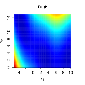
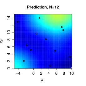
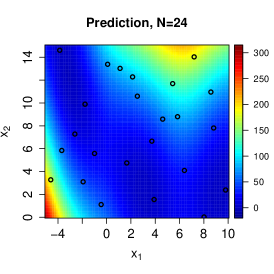
Constructing a GP emulator to approximate computer simulation typically starts with a “space-filling” design, such as the Latin hypercube sampling (LHS), to fill the input space. Numerical solutions of computer models were then obtained at these design points, and the set is used for training a GP emulator. For any observed input , the predictive mean in (4) is often used for predictions, and the uncertainty of observations can be obtained through the predictive distribution. in Figure 1, we plot the predictive mean of a GP emulator to approximate the Branin function [56] with N training inputs sampled from LHS, using the default setting of the RobustGaSP package [18]. When the number of observations increases from (middle panel) to (right panel), the predictive error becomes smaller.
|
The computational complexity of GP models increases at the order of , which prohibits applications on emulating complex computer simulations, when a relatively large number of simulation runs are required. In the next section, we will introduce the state space representation of GP with Matérn covariance and one-dimensional input, where the computational order scales as without approximation. This method can be applied to problems with high dimensional input space discussed in Section 4.
3 Marginalization in Kalman filter
3.1 State space representation of GP with the Matérn kernel
Suppose we model the observations by Equation (8) where the latent process is assumed to follow a GP on 1D input. For simplicity, here we assume a zero mean parameter (), and a mean function can be easily included in the analysis. It has been realized that a GP defined in 1D input space using a Matérn covariance with a half-integer roughness parameter input can be written as stochastic differential equations (SDEs) [63, 22], which can reduce the operations of computing the likelihood and making predictions from to operations, with the use of Kalman filter. Here we first review SDE representation and then we discuss marginalization of latent variables in the Kalman filter algorithm for scalable computation.
When the roughness parameter is , for instance, the Matérn kernel has the expression below
| (9) |
where is the distance between any and is a range parameter typically estimated by data. The output and two derivatives of the GP with the Matérn kernel in (9) can be written as the SDE below,
| (10) |
or in the matrix form,
where , with , and is the th derivative of the process . Denote and . Assume the 1D input is ordered, i.e. . The solution of SDE in (10) can be expressed as a continuous-time dynamic linear model [61],
| (11) | ||||
where for , and Gaussian noise follows . Here and from , and stationary distribution , with Both and have closed-form expressions given in the Appendix 5.1. The joint distribution of the states follows , where the inverse covariance is a block tri-diagonal matrix discussed in Appendix 5.1.
3.2 Kalman filter as a scalable marginalization technique
For dynamic linear models in (11), Kalman filter and Rauch–Tung–Striebel (RTS) smoother can be used as an exact and scalable approach to compute the likelihood, and predictive distributions. The Kalman filter and RTS smoother are sometimes called the forward filtering and backward smoothing/sampling algorithm, widely used in dynamic linear models of time series. We refer the readers to [61, 41] for discussion of dynamic linear models.
Write , , and for . In Lemma 1, we summarize Kalman filter and RTS smoother for the dynamic linear model in (11). Compared with computational operations and storage cost from GPs, the outcomes of Kalman filter and RTS smoother can be used for computing the likelihood and predictive distribution with operations and storage cost, summarized in Lemma 1. All the distributions in Lemma 1 and Lemma 2 are conditional distributions given parameters , which are omitted for simplicity.
Lemma 1 (Kalman Filter and RTS Smoother [26, 45]).
1. (Kalman Filter.) Let . For , iteratively we have,
-
(i)
the one-step-ahead predictive distribution of given ,
(12) with and ,
-
(ii)
the one-step-ahead predictive distribution of given ,
(13) with and ,
-
(iii)
the filtering distribution of given ,
(14) with and .
2. (RTS Smoother.) Denote , then recursively for ,
| (15) |
where and .
Lemma 2 (Likelihood and predictive distribution).
1. (Likelihood.) The likelihood follows
where and are given in Kalman filter. The likelihood can be used to obtain the MLE of the parameters .
2. (Predictive distribution.)
-
(i)
By the last step of Kalman filter, one has and recursively by the RTS smoother, the predictive distribution of for follows
(16) - (ii)
Although we introduce the Matérn kernel with as an example, the likelihood and predictive distribution of GPs with the Matérn kernel of a small half-integer roughness parameter can be computed efficiently, for both equally spaced and not equally spaced 1D inputs. For the Matérn kernel with a very large roughness parameter, the dimension of the latent states becomes large, which makes efficient computation prohibitive. In practice, the Matérn kernel with a relatively large roughness parameter (e.g. with ) is found to be accurate for estimating a smooth latent function in computer experiments [20, 2]. Because of this reason, the Matérn kernel with is the default choice of the kernel function in some packages of GP emulators [47, 18].
For a model containing latent variables, one may proceed with two usual approaches:
-
(i)
sampling the latent variables from the posterior distribution by the MCMC algorithm,
-
(ii)
optimizing the latent variables to minimize a loss function.
For approach (i), the MCMC algorithm is usually much slower than the Kalman filter, as the number of the latent states is high, requiring a large number of posterior samples [17]. On the other hand, the prior correlation between states may not be taken into account directly in approach (ii), making the estimation less efficient than the Kalman filter, if data contain correlation across latent states. In comparison, the latent states in the dynamic linear model in (11) are iteratively marginalized out in Kalman filter, and the closed-form expression is derived in each step, which only takes operations and storage cost, with being the number of observations.
In practice, when a sensible probability model or a prior of latent variables is considered, the principle is to integrate out the latent variables when making predictions. Posterior samples and optimization algorithms, on the other hand, can be very useful for approximating the marginal likelihood when closed-form expressions are not available. As an example, we will introduce applications that integrate the sparse covariance structure along with conjugate gradient optimization into estimating particle interaction kernels, and forecasting particle trajectories in Section 4, which integrates both marginalization and optimization to tackle a computationally challenging scenario.
|
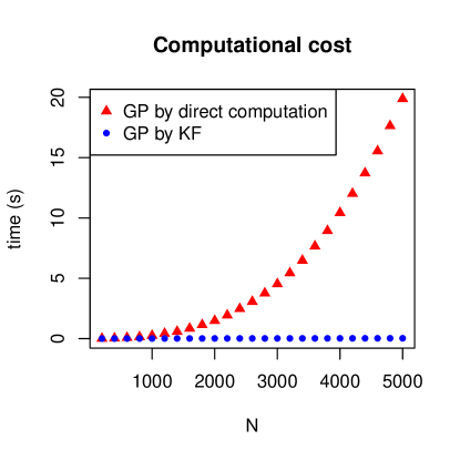
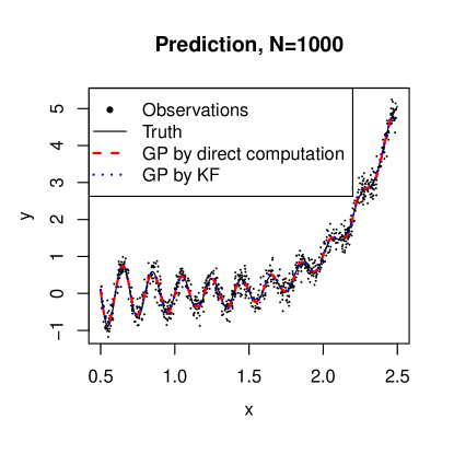
In Figure 2, we compare the cost for computing the predictive mean for a nonlinear function with 1D inputs [16]. The input is uniformly sampled from , and an independent Gaussian white noise with a standard deviation of is added in simulating the observations. We compare two ways of computing the predictive mean. The first approach implements direct computation of the predictive mean by Equation (5). The second approach is computed by the likelihood function and predictive distribution from Lemma 2 based on the Kalman filter and RTS smoother. The range and nugget parameters are fixed to be and for demonstration purposes, respectively. The computational time of this simulated experiment is shown in the left panel in Figure 2. The approach based on Kalman filter and RTS smoother is much faster, as computing the likelihood and making predictions by Kalman filter and RTS smoother only require operations, whereas the direct computation cost operations. The right panel gives the predictive mean, latent truth, and observations, when . The difference between the two approaches is very small, as both methods are exact.
3.3 Marginalization of correlated matrix observations with multi-dimensional inputs
The Kalman filter is widely applied in signal processing, system control, and modeling time series. Here we introduce a few recent studies that apply Kalman filter to GP models with Matérn covariance to model spatial, spatio-temporal, and functional observations.
Let be an -dimensional real-valued output vector at a -dimensional input vector . For simplicity, assume the mean is zero. Consider the latent factor model:
| (17) |
where is an factor loading matrix and is a -dimensional factor processes, with . The noise process follows . Each factor is modeled by a zero-mean Gaussian process (GP), meaning that follows a multivariate normal distribution , where the entry of is parameterized by a covariance function for . The model (17) is often known as the semiparametric latent factor model in the machine learning community [53], and it belongs to a class of linear models of coregionalization [3]. It has a wide range of applications in modeling multivariate spatially correlated data and functional observations from computer experiments [14, 25, 40].
We have the following two assumptions for model (17).
Assumption 1.
The prior of latent processes and are independent, for any .
Assumption 2.
The factor loadings are orthogonal, i.e. .
The first assumption is typically assumed for modeling multivariate spatially correlated data or computer experiments [3, 25]. Secondly, note that the model in (17) is unchanged if we replace by for an invertible matrix , meaning that the linear subspace of can be identified if no further constraint is imposed. Furthermore, as the variance of each latent process is estimated by the data, imposing the unity constraint on each column of can reduce identifiability issues. The second assumption was also assumed in other recent studies [31, 30].
Given Assumption 1 and Assumption 2, we review recent results that alleviates the computational cost. Let us first assume the observations are an matrix .
Lemma 3 (Posterior independence and orthogonal projection [17]).
1. (Posterior Independence.) For any
and for each ,
where , and with .
2. (Orthogonal projection.) After integrating , the marginal likelihood is a product of multivariate normal densities at projected observations:
| (18) |
where with being the th column of , the orthogonal component of , and denotes the density for a multivariate normal distribution.
The properties in Lemma 17 lead to computationally scalable expressions of the maximum marginal likelihood estimator (MMLE) of factor loadings.
Theorem 1 (Generalized probabilistic principal component analysis [19]).
Assume , after marginalizing out for , we have the results below.
-
•
If , the marginal likelihood is maximized when
(19) where is an matrix of the first principal eigenvectors of and is a orthogonal rotation matrix;
-
•
If the covariances of the factor processes are different, denoting , the MMLE of factor loadings is
(20)
The estimator in Theorem 1 is called the generalized probabilistic principal component analysis (GPPCA). The optimization algorithm that preserves the orthogonal constraints in (20) is available in [60].
In [58], the latent factor is assumed to follow independent standard normal distributions, and the authors derived the MMLE of the factor loading matrix , which was termed the probabilistic principal component analysis (PPCA). The GPPCA extends the PPCA to correlated latent factors modeled by GPs, which incorporates the prior correlation information between outputs as a function of inputs, and the latent factor processes were marginalized out when estimating the factor loading matrix and other parameters. When the input is 1D and the Matérn covariance is used for modeling latent factors, the computational order of GPPCA is , which is the same as the PCA. For correlated data, such as spatio-temporal observations and multivariate functional data, GPPCA provides a flexible and scalable approach to estimate factor loading by marginalizing out the latent factors [19].
Spatial and spatio-temporal models with a separable covariance can be written as a special case of the model in (17). For instance, suppose and the latent factor matrix follows where and are and subcovariances, respectively. Denote the eigen decomposition with being a diagonal matrix with the eigenvalues , for . Then this separable model can be written as the model in (17), with , . The connection suggests that the latent factor loading matrix can be specified as the eigenvector matrix of a covariance matrix, parameterized by a kernel function. This approach is studied in [17] for modeling incomplete lattice with irregular missing patterns, and the Kalman filter is integrated for accelerating computation on massive spatial and spatio-temporal observations.
4 Scalable marginalization for learning particle interaction kernels from trajectory data
Collective motions with particle interactions are very common in both microscopic and macroscopic systems [35, 36]. Learning interaction kernels between particles is important for two purposes. First, physical laws are less understood for many complex systems, such as cell migration or non-equilibrium thermodynamic processes. Estimating the interaction kernels between particles from fields or experimental data is essential for learning these processes. Second, simulation of particle interactions, such as ab initio molecular dynamics simulation, can be very computationally expensive. Statistical learning approaches can be used for reducing the computational cost of simulations.
For demonstration purposes, we consider a simple first-order system. In [34], for a system with interacting particles, the velocity of the th particle at time , , is modeled by positions between all particles,
| (21) |
where is a latent interaction kernel function between particle and all other particles, with being the Euclidean distance, and is a vector of differences between positions of particles and , for . Here is a two-body interaction function. In molecular dynamics simulation, for instance, the Lennard-Jones potential can be related to molecular forces and the acceleration of molecules in a second-order system. The statistical learning approach can be extended to a second-order system that involves acceleration and external force terms. The first-order system as (21) can be considered as an approximation of the second-order system. Furthermore, the interaction between particles is global, as any particle is affected by all other particles. Learning global interactions is more computationally challenging than local interactions [51], and approximating the global interaction by the local interaction is of interest in future studies.
One important goal is to efficiently estimate the unobservable interaction functions from the particle trajectory data, without specifying a parametric form. This goal is key for estimating the behaviors of dynamic systems in experiments and in observational studies, as the physics law in a new system may be unknown. In [13], is modeled by a zero-mean Gaussian process with a Matérn covariance:
| (22) |
Computing estimation of interactions of large-scale systems or more simulation runs, however, is prohibitive, as the direct inversion of the covariance matrix of observations of velocities requires operations, where is the number of simulations or experiments, is the number of particles, is the dimension of each particle, denotes the number of time points for each trial. Furthermore, constructing such covariance contains computing an matrix of for a -dimensional input space, which takes operations. Thus, directly estimating interaction kernel with a GP model in (22) is only applicable to systems with a small number of observations [34, 13].
This work makes contributions from two different aspects for estimating dynamic systems of interacting particles. We first show the covariance of velocity observations can be obtained by operations on a few sparse matrices, after marginalizing out the latent interaction function. The sparsity of the inverse covariance of the latent interaction kernel allows us to modify the Kalman filter to efficiently compute the matrix product in this problem, and then apply a conjugate gradient (CG) algorithm [24, 21, 49] to solve this system iteratively. The computational complexity of computing the predictive mean and variance of a test point is at the order of , for a system of particles, observations, and is the number of iterations required in the CG algorithm. We found that typically around a few hundred CG iterations can achieve high predictive accuracy for a moderately large number of observations. The algorithm leads substantial reduction of computational cost, compared to direct computation.
Second, we study the effect of experimental designs on estimating the interaction kernel function. In previous studies, it is unclear how initial positions, time steps of trajectory and the number of particles affect the accuracy in estimating interaction kernels. Compared to other conventional problems in computer model emulation, where a “space-filling” design is often used, here we cannot directly observe the realizations of the latent function. Instead, the output velocity is a weighted average of the interaction kernel functions between particles. Besides, we cannot directly control distances between the particles moving away from the initial positions, in both simulation and experimental studies. When the distance between two particles and is small, the contribution can be small, if the repulsive force by does not increase as fast as the distance decreases. Thus we found that the estimation of interaction kernel function can be less accurate in the input domain of small distances. This problem can be alleviated by placing initial positions of more particles close to each other, providing more data with small distance pairs that improve the accuracy in estimation.
4.1 Scalable computation based on sparse representation of inverse covariance
For illustration purposes, let us first consider a simple scenario where we have simulation and time point of a system of interacting particles at a dimensional space. Since we only have 1 time point, we omit the notation when there is no confusion. The algorithm for the general scenario with and is discussed in Appendix 5.2. In practice, the experimental observations of velocity from multiple particle tracking algorithms or particle image velocimetry typically contain noises [1]. Even for simulation data, the numerical error could be non-negligible for large and complex systems. In these scenarios, the observed velocity is a noisy realization: , where denotes a vector of Gaussian noise with variance .
Assume the observations of velocity are . After integrating out the latent function modeled in Equation (22), the marginal distribution of observations follows
| (23) |
where is an block diagonal matrix, with the th block in the diagonals being , and is an matrix, where the term in the th block is with and for . Direct computation of the likelihood involves computing the inverse of an covariance matrix and constructing an matrix , which costs operations. This is computationally expensive even for small systems.
Here we use an exponential kernel function, with range parameter , of modeling any nonnegative distance input for illustration, where this method can be extended to include Matérn kernels with half-integer roughness parameters. Denote distance pairs , and there are unique positive distance pairs. Denote the distance pairs in an increasing order with the subscript meaning ‘sorted’. Here we do not need to consider the case when , as , leading to zero contribution to the velocity. Thus the model in (21) can be reduced to exclude the interaction between particle at zero distance. In reality, two particles at the same position are impractical, as there typically exists a repulsive force when two particles get very close. Hence, we can reduce the distance pairs for and , to unique positive terms in an increasing order, for .
Denote the correlation matrix of the kernel outputs by and is sparse matrix with nonzero terms on each row, where the nonzero entries of the th particle correspond to the distance pairs in the . Denote the nugget parameter . After marginalizing out , the covariance of velocity observations follows
| (24) |
with
| (25) |
The conditional distribution of the interaction kernel at any distance follows
| (26) |
where the predictive mean and variance follow
| (27) | ||||
| (28) |
with . After obtaining the estimated interaction kernel, one can use it to forecast trajectories of particles and understand the physical mechanism of flocking behaviors.
Our primary task is to efficiently compute the predictive distribution of interaction kernel in (26), where the most computationally expensive terms in the predictive mean and variance is and . Note that the is a sparse matrix with nonzero terms and the inverse covariance matrix is a tri-diagonal matrix. However, directly applying the CG algorithm is still computationally challenging, as neither nor is sparse. To solve this problem, we extend a step in the Kalman filter to efficiently compute the matrix-vector multiplication with the use of sparsity induced by the choice of covariance matrix. Each step of the CG iteration in the new algorithm only costs operations for computing a system of particles and dimensions with CG iteration steps. For most systems we explored, we found a few hundred iterations in the CG algorithm achieve high accuracy. The substantial reduction of the computational cost allows us to use more observations to improve the predictive accuracy. We term this approach the sparse conjugate gradient algorithm for Gaussian processes (sparse CG-GP). The algorithm for the scenario with simulations, each containing time frames of particles in a dimensional space, is discussed in Appendix 5.2.
|
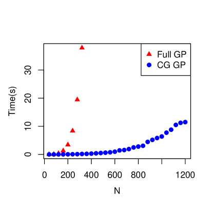
The comparison of the computational cost between the full GP model and the proposed sparse CG-GP method is shown in the right panel in Figure 3. The most computational expensive part of the full GP model is on constructing the correlation matrix of for distance pairs. The sparse CG-GP algorithm is much faster as we do not need to construct this covariance matrix; instead we only need to efficiently compute matrix multiplication by utilizing the sparse structure of the inverse of (Appendix 5.2). Note the GP model with an exponential covariance naturally induces a sparse inverse covariance matrix that can be used for faster computation, which is different from imposing a sparse covariance structure for approximation.
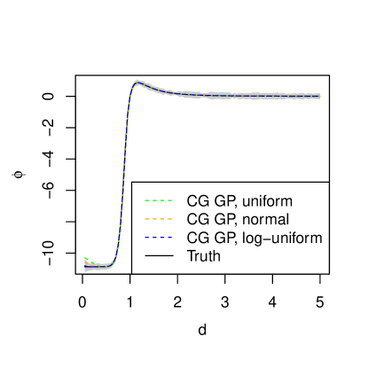
In the left panel in Figure 3, we show the predictive mean and uncertainty assessment by the sparse CG-GP method for three different designs for sampling the initial positions of particles. From the first to the third designs, the initial value of each coordinate of the particle is sampled independently from a uniform distribution , normal distribution , and log uniform (reciprocal) distribution , respectively.
For experiments with the interaction kernel being the truncated Lennard-Jones potential given in Appendix 5.2, we use , , , , and for three designs of initial positions. Compared with the first design, the second design of initial positions, which was assumed in [34], has a larger probability mass of distributions near 0. In the third design, the distributions of the distance between particle pairs are monotonically decreasing, with more probability mass near 0 than those in the first two designs. In all cases shown in Figure 3, we assume , and the noise variance is set to be in the simulation. For demonstration purposes, the range and nugget parameters are fixed to be and respectively, when computing the predictive distribution of . The estimation of the interaction kernel on large distances is accurate for all different designs, whereas the estimation of the interaction kernel at small distances is not satisfying for the first two designs. When particles are initialized from the third design (log-uniform), the accuracy is better, as there are more particles near each other, providing more information about the particles at small values. This result is intuitive, as the small distance pairs have relatively small contributions to the velocity based on Equation (21), and we need more particles close to each other to estimate the interaction kernel function at small distances.
The numerical comparison between different designs allows us to better understand the learning efficiency in different scenarios, which can be used to design experiments. Because of the large improvement of computational scalability compared to previous studies [13, 34], we can accurately estimate interaction kernels based on more particles and longer trajectories.
4.2 Numerical results
Here we discuss two scenarios, where the interaction between particles follow the truncated Lennard-Jones (LJ) and opinion dynamics (OD) kernel functions. The LJ potential is widely used in MD simulations of interacting molecules [43]. First-order systems of form (21) have also been successfully applied in modeling opinion dynamics in social networks (see the survey [36] and references therein). The interaction function models how the opinions of pairs of people influence each other. In our numerical example, we consider heterophilious opinion interactions: each agent is more influenced by its neighbors slightly further away from its closest neighbors. As time evolves, the opinions of agents merge into clusters, with the number of clusters significantly smaller than the number of agents. This phenomenon was studied in [36] that heterophilious dynamics enhances consensus, contradicting the intuition that would suggest that the tendency to bond more with those who are different rather than with those who are similar would break connections and prevent clusters of consensus.
The details of the interaction functions are given in Appendix 5.3. For each interaction, we test our method based on 12 configurations of 2 particle sizes ( and ), 2 time lengths ( and ), and 3 designs of initial positions (uniform, normal and log-uniform). The computational scalability of the sparse CG algorithm allows us to efficiently compute the predictions in most of these experimental settings within a few seconds. For each configuration, we repeat the experiments 10 times to average the effects of randomness in the initial positions of particles. The root of the mean squared error in predicting the interaction kernels by averaging these 10 experiments of each configuration is given in Appendix 5.4.
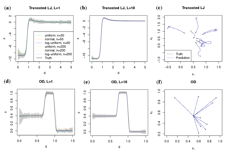
In Figure 4, we show the estimation of interactions kernels and forecasts of particle trajectories with different designs, particle sizes and time points. The sparse CG-GP method is relatively accurate for almost all scenarios. Among different initial positions, the estimation of trajectories for LJ interaction is the most accurate when the initial positions of the particles are sampled by the log-uniform distribution. This is because there are more small distances between particles when the initial positions follow a log-uniform distribution, providing more data to estimate the interaction kernel at small distances. Furthermore, when we have more particles or observations at larger time intervals, the estimation of the interaction kernel from all designs becomes more accurate in terms of the normalized root mean squared error with the detailed comparison given in Appendix 5.4.
In panel (c) and panel (f) of Figure 4, we plot the trajectory forecast of particles over time points for the truncated LJ kernel and OD kernel, respectively. In both simulation scenarios, interaction kernels are estimated based on trajectories of particles across time steps with initial positions sampled from the log-uniform design. The trajectories of only particles out of particles are shown for better visualization. For trajectories simulated by the truncated LJ, some particles can move very close, since the repulsive force between two particles becomes smaller as the force is proportional to the distance from Equation (21), and the truncation of kernel substantially reduces the repulsive force when particles move close. For the OD simulation, the particles move toward a cluster, as expected, since the particles always have attractive forces between each other. The forecast trajectories are close to the hold-out truth, indicating the high accuracy of our approach.
Compared with the results shown in previous studies [34, 13], estimating the interaction kernels and forecasting trajectories both look more accurate. The large computational reduction by the sparse CG-GP algorithm shown in Figure 3 permits the use of longer trajectories from more particles to estimate the interaction kernel, which improves the predictive accuracy. Here particle has interactions with all other particles in our simulation, making the number of distance pairs large. Yet we are able to estimate the interaction kernel and forecast the trajectories of particles within only tens of seconds in a desktop for the most time consuming scenario we considered. Since the particles typically have very small or no interaction when the distances between them are large, approximation can be made by enforcing interactions between particles within the specified radius, for further reducing the computational cost.
5 Concluding remarks
We have introduced scalable marginalization of latent variables for correlated data. We first introduce GP models and reviewed the SDE representation of GPs with Matérn covariance and one-dimensional input. Kalman filter and RTS smoother were introduced as a scalable marginalization way to compute the likelihood function and predictive distribution, which reduces the computational complexity of GP with Matérn covariance for 1D input from to operations without approximation, where is the number of observations. Recent efforts on extending scalable computation from 1D input to multi-dimensional input are discussed. In particular, we developed a new scalable algorithm for predicting particle interaction kernel and forecast trajectories of particles. The achievement is through the sparse representation of GPs in modeling interaction kernel, and then efficient computation for matrix multiplication by modifying the Kalman filter algorithm. An iterative algorithm based on CG can then be applied, which reduces the computational complexity.
There are a wide range of future topics relevant to this study. First, various models of spatio-temporal data can be written as random factor models in (17) with latent factors modeled as Gaussian processes for temporal inputs. It is of interest to utilize the computational advantage of the dynamic linear models of factor processes, extending the computational tools by relaxing the independence between prior factor processes in Assumption 1 or incorporating the Toeplitz covariance structure for stationary temporal processes. Second, for estimating systems of particle interactions, we can further reduce computation by only considering interactions within a radius between particles. Third, a comprehensively study the experimental design, initialization, and parameter estimation in will be helpful for estimating latent interaction functions that can be unidentifiable or weakly identifiable in certain scenarios. Furthermore, velocity directions and angle order parameters are essential for understanding the mechanism of active nematics and cell migration, which can motivate more complex models of interactions. Finally, the sparse CG algorithm developed in this work is of interest to reducing the computational complexity of GP models with multi-dimensional input and general designs.
Acknowledgement
The work is partially supported by the National Institutes of Health under Award No. R01DK130067. Gu and Liu acknowledge the partial support from National Science Foundation (NSF) under Award No. DMS-2053423. Fang acknowledges the support from the UCSB academic senate faculty research grants program. Tang is partially supported by Regents Junior Faculty fellowship, Faculty Early Career Acceleration grant, Hellman Family Faculty Fellowship sponsored by UCSB and the NSF under Award No. DMS-2111303. The authors thank the editor and two referees for their comments that substantially improved the article.
Appendix
5.1 Closed-form expressions of state space representation of GP having Matérn covariance with
Denote , and . For , and in (11) have the expressions below:
with
and the stationary covariance of , , is
The joint distribution of latent states follows , where the is a symmetric block tri-diagonal matrix with the th diagonal block being for , and the th diagonal block being . The primary off-diagonal block of is , for .
Suppose . Let and . The “*” terms and can be computed by replacing in and by , whereas the “*” terms and can be computed by replacing the in and by . Furthermore, .
5.2 The sparse CG-GP algorithm for estimating interaction kernels
Here we discuss the details of computing the predictive mean and variance in (26). The -vector of velocity observations is denoted as , where the total number of observations is defined by . To compute the predictive mean and variance, the most computational challenging part is to compute -vector . Here and are and , respectively, where is the number of non-zero unique distance pairs. Note that both and are sparse. Instead of directly computing the matrix inversion and the matrix-vector multiplication, we utilize the sparsity structure to accelerate the computation in the sparse CG-GP algorithm. In the iteration, we need to efficiently compute
| (29) |
for any real-valued N-vector .
We have four steps to compute the quantity in (29) efficiently. Denote the th spatial coordinate of particle at time , in the th simulation, for , , and . In the following, we use to denote a vector of all positions in the th simulation and vice versa. Furthermore, we use to mean the th entry of any vector , and to mean the th row vector and th column vector of any matrix , respectively. The rank of a particle with position is defined to be .
First, we reduce the sparse matrix of distance difference pairs to an matrix , where ‘re’ means reduced, with the th entry of being , for any , and . Furthermore, we create a matrix in which the th row records the rank of a distance pair is the th largest in the zero-excluded sorted distance pairs , where and are the rank of rows of these distances in the matrix , where the th column records the unordered distance pairs of the th particle for . We further assume .
For any -vector , the th entry of can be written as
| (30) |
where for , if the th largest entry of distance pair is from time frame in the th simulation. The output is denoted as an vector , i.e. .
Second, since the exponential kernel is used, is a tri-diagonal matrix [20]. We modify a Kalman filter step to efficiently compute the product of an upper bi-diagonal , where is the factor of the Cholesky decomposition . Denote the Cholesky decomposition of the inverse covariance the factor , where can be written as the lower bi-diagonal matrix below:
| (31) |
where for . We modify the Thomas algorithm [57] to solve from equation . Here is an upper bi-diagonal matrix with explicit form
| (32) |
Here only up to 2 entries in each row of are nonzero. Using a backward solver, the can be obtained by the iteration below:
| (33) | ||||
| (34) |
for . Note that the Thomas algorithm is not stable in general, but here the stability issue is greatly improved, as the matrix in the system is bi-diagonal instead of tri-diagonal.
Third, we compute by solving :
| (35) | ||||
| (36) |
for .
Finally, we denote a matrix . is initialized as a zero matrix. And then for , row of stores the ranks of distances between the th particle and other particles in . For instance, at the th time step in the th simulation, particle has non-zero distances with ranks in . Then the th row of is filled with .
Given any -vector , the th entry of can be written as
| (37) |
assuming that satisfies and for some and , and . The output of this step is an vector , with the th entry being , for .
We summarize the sparse CG-GP algorithm using the following steps to compute in (29) below.
5.3 Interaction kernels in simulated studies
Here we give the expressions of the truncated L-J and OD kernels of particle interaction in [34, 13]. The truncated LJ kernel is given by
where
with and .
The interaction kernel of OD is defined as
where and .
5.4 Further numerical results on estimating interaction kernels
We outline the numerical results of estimating the interaction functions at equally spaced distance pairs at and for the truncated LJ and OD, respectively. For each configuration, we repeat the simulation times and compute the predictive error in each simulation. The total number of test points is . For demonstration purposes, we do not add a noise into the simulated data (i.e. ). The range and nugget parameters are fixed to be and . We compute the normalized root of mean squared error (NRMSE) in estimating the interaction kernel function:
where is the estimated interaction kernel from the velocities and positions of the particles; is the standard deviation of the interaction function at test points.
| Truncated LJ | n=50 | n=200 | n=50 | n=200 |
|---|---|---|---|---|
| L=1 | L=1 | L=10 | L=10 | |
| Uniform | ||||
| Normal | ||||
| Log-uniform | ||||
| OD | n=50 | n=200 | n=50 | n=200 |
| L=1 | L=1 | L=10 | L=10 | |
| Uniform | ||||
| Normal | ||||
| Log-uniform |
Table 1 gives the NRMSE of the sparse CG-GP method for the truncated LJ and OD kernels at 12 configurations. Typically the estimation is the most accurate when the initial positions of the particles are sampled from the log-uniform design for a given number of observations and an interaction kernel. This is because the contributions to the velocities from the kernel function are proportional to the distance of particle in (21), and small contributions from the interaction kernel at small distance values make the kernel hard to estimate from the trajectory data in general. When the initial positions of the particles are sampled from the log-uniform design, more particles are close to each other, which provides more information to estimate the interaction kernel at a small distance.
Furthermore, the predictive error of the interaction kernel is smaller, when the trajectories with a larger number of particle sizes or at longer time points are used in estimation, as more observations typically improve predictive accuracy. The sparse CG-GP algorithm reduces the computational cost substantially, which allows more observations to be used for making predictions.
References
- [1] Ronald J Adrian and Jerry Westerweel. Particle image velocimetry. Number 30. Cambridge university press, 2011.
- [2] Kyle R Anderson, Ingrid A Johanson, Matthew R Patrick, Mengyang Gu, Paul Segall, Michael P Poland, Emily K Montgomery-Brown, and Asta Miklius. Magma reservoir failure and the onset of caldera collapse at Kīlauea volcano in 2018. Science, 366(6470), 2019.
- [3] Sudipto Banerjee, Bradley P Carlin, and Alan E Gelfand. Hierarchical modeling and analysis for spatial data. Crc Press, 2014.
- [4] Maria Maddalena Barbieri and James O Berger. Optimal predictive model selection. The annals of statistics, 32(3):870–897, 2004.
- [5] Maria J Bayarri, James O Berger, Rui Paulo, Jerry Sacks, John A Cafeo, James Cavendish, Chin-Hsu Lin, and Jian Tu. A framework for validation of computer models. Technometrics, 49(2):138–154, 2007.
- [6] James O Berger, Victor De Oliveira, and Bruno Sansó. Objective Bayesian analysis of spatially correlated data. Journal of the American Statistical Association, 96(456):1361–1374, 2001.
- [7] James O Berger, Brunero Liseo, and Robert L Wolpert. Integrated likelihood methods for eliminating nuisance parameters. Statistical science, 14(1):1–28, 1999.
- [8] James O Berger and Luis R Pericchi. The intrinsic bayes factor for model selection and prediction. Journal of the American Statistical Association, 91(433):109–122, 1996.
- [9] Iain D Couzin, Jens Krause, Nigel R Franks, and Simon A Levin. Effective leadership and decision-making in animal groups on the move. Nature, 433(7025):513–516, 2005.
- [10] Noel Cressie and Gardar Johannesson. Fixed rank kriging for very large spatial data sets. Journal of the Royal Statistical Society: Series B (Statistical Methodology), 70(1):209–226, 2008.
- [11] Abhirup Datta, Sudipto Banerjee, Andrew O Finley, and Alan E Gelfand. Hierarchical nearest-neighbor gaussian process models for large geostatistical datasets. Journal of the American Statistical Association, 111(514):800–812, 2016.
- [12] Bruno De Finetti. La prévision: ses lois logiques, ses sources subjectives. In Annales de l’institut Henri Poincaré, volume 7, pages 1–68, 1937.
- [13] Jinchao Feng, Yunxiang Ren, and Sui Tang. Data-driven discovery of interacting particle systems using gaussian processes. arXiv preprint arXiv:2106.02735, 2021.
- [14] Alan E Gelfand, Sudipto Banerjee, and Dani Gamerman. Spatial process modelling for univariate and multivariate dynamic spatial data. Environmetrics: The official journal of the International Environmetrics Society, 16(5):465–479, 2005.
- [15] Robert B Gramacy and Daniel W Apley. Local Gaussian process approximation for large computer experiments. Journal of Computational and Graphical Statistics, 24(2):561–578, 2015.
- [16] Robert B Gramacy and Herbert KH Lee. Cases for the nugget in modeling computer experiments. Statistics and Computing, 22(3):713–722, 2012.
- [17] Mengyang Gu and Hanmo Li. Gaussian Orthogonal Latent Factor Processes for Large Incomplete Matrices of Correlated Data. Bayesian Analysis, pages 1 – 26, 2022.
- [18] Mengyang Gu, Jesus Palomo, and James O. Berger. RobustGaSP: Robust Gaussian Stochastic Process Emulation in R. The R Journal, 11(1):112–136, 2019.
- [19] Mengyang Gu and Weining Shen. Generalized probabilistic principal component analysis of correlated data. Journal of Machine Learning Research, 21(13), 2020.
- [20] Mengyang Gu, Xiaojing Wang, and James O Berger. Robust Gaussian stochastic process emulation. Annals of Statistics, 46(6A):3038–3066, 2018.
- [21] Wolfgang Hackbusch. Iterative solution of large sparse systems of equations, volume 95. Springer, 1994.
- [22] Jouni Hartikainen and Simo Sarkka. Kalman filtering and smoothing solutions to temporal gaussian process regression models. In Machine Learning for Signal Processing (MLSP), 2010 IEEE International Workshop on, pages 379–384. IEEE, 2010.
- [23] Silke Henkes, Yaouen Fily, and M Cristina Marchetti. Active jamming: Self-propelled soft particles at high density. Physical Review E, 84(4):040301, 2011.
- [24] Magnus R Hestenes and Eduard Stiefel. Methods of conjugate gradients for solving. Journal of research of the National Bureau of Standards, 49(6):409, 1952.
- [25] Dave Higdon, James Gattiker, Brian Williams, and Maria Rightley. Computer model calibration using high-dimensional output. Journal of the American Statistical Association, 103(482):570–583, 2008.
- [26] Rudolph Emil Kalman. A new approach to linear filtering and prediction problems. Journal of basic Engineering, 82(1):35–45, 1960.
- [27] Matthias Katzfuss and Joseph Guinness. A general framework for vecchia approximations of gaussian processes. Statistical Science, 36(1):124–141, 2021.
- [28] Hannes Kazianka and Jürgen Pilz. Objective Bayesian analysis of spatial data with uncertain nugget and range parameters. Canadian Journal of Statistics, 40(2):304–327, 2012.
- [29] Balaji Lakshminarayanan, Alexander Pritzel, and Charles Blundell. Simple and scalable predictive uncertainty estimation using deep ensembles. Advances in neural information processing systems, 30, 2017.
- [30] Clifford Lam and Qiwei Yao. Factor modeling for high-dimensional time series: inference for the number of factors. The Annals of Statistics, 40(2):694–726, 2012.
- [31] Clifford Lam, Qiwei Yao, and Neil Bathia. Estimation of latent factors for high-dimensional time series. Biometrika, 98(4):901–918, 2011.
- [32] Jaehoon Lee, Yasaman Bahri, Roman Novak, Samuel S Schoenholz, Jeffrey Pennington, and Jascha Sohl-Dickstein. Deep neural networks as gaussian processes. arXiv preprint arXiv:1711.00165, 2017.
- [33] Finn Lindgren, Håvard Rue, and Johan Lindström. An explicit link between gaussian fields and gaussian markov random fields: the stochastic partial differential equation approach. Journal of the Royal Statistical Society: Series B (Statistical Methodology), 73(4):423–498, 2011.
- [34] Fei Lu, Ming Zhong, Sui Tang, and Mauro Maggioni. Nonparametric inference of interaction laws in systems of agents from trajectory data. Proc. Natl. Acad. Sci. U.S.A., 116(29):14424–14433, 2019.
- [35] M Cristina Marchetti, Jean-François Joanny, Sriram Ramaswamy, Tanniemola B Liverpool, Jacques Prost, Madan Rao, and R Aditi Simha. Hydrodynamics of soft active matter. Reviews of modern physics, 85(3):1143, 2013.
- [36] Sebastien Motsch and Eitan Tadmor. Heterophilious dynamics enhances consensus. SIAM review, 56(4):577–621, 2014.
- [37] Joseph Muré. Propriety of the reference posterior distribution in gaussian process modeling. The Annals of Statistics, 49(4):2356–2377, 2021.
- [38] Radford M Neal. Bayesian learning for neural networks, volume 118. Springer Science & Business Media, 2012.
- [39] Rui Paulo. Default priors for Gaussian processes. Annals of statistics, 33(2):556–582, 2005.
- [40] Rui Paulo, Gonzalo García-Donato, and Jesús Palomo. Calibration of computer models with multivariate output. Computational Statistics and Data Analysis, 56(12):3959–3974, 2012.
- [41] Giovanni Petris, Sonia Petrone, and Patrizia Campagnoli. Dynamic linear models with R. Springer, 2009.
- [42] Adrian E Raftery, David Madigan, and Jennifer A Hoeting. Bayesian model averaging for linear regression models. Journal of the American Statistical Association, 92(437):179–191, 1997.
- [43] Dennis C Rapaport and Dennis C Rapaport Rapaport. The art of molecular dynamics simulation. Cambridge university press, 2004.
- [44] Carl Edward Rasmussen. Gaussian processes for machine learning. MIT Press, 2006.
- [45] Herbert E Rauch, F Tung, and Charlotte T Striebel. Maximum likelihood estimates of linear dynamic systems. AIAA journal, 3(8):1445–1450, 1965.
- [46] Cuirong Ren, Dongchu Sun, and Chong He. Objective bayesian analysis for a spatial model with nugget effects. Journal of Statistical Planning and Inference, 142(7):1933–1946, 2012.
- [47] Olivier Roustant, David Ginsbourger, and Yves Deville. Dicekriging, diceoptim: Two r packages for the analysis of computer experiments by kriging-based metamodeling and optimization. Journal of Statistical Software, 51(1):1–55, 2012.
- [48] Håvard Rue, Sara Martino, and Nicolas Chopin. Approximate bayesian inference for latent gaussian models by using integrated nested laplace approximations. Journal of the royal statistical society: Series B (statistical methodology), 71(2):319–392, 2009.
- [49] Yousef Saad. Iterative methods for sparse linear systems. SIAM, 2003.
- [50] Jerome Sacks, William J Welch, Toby J Mitchell, and Henry P Wynn. Design and analysis of computer experiments. Statistical science, 4(4):409–423, 1989.
- [51] Alvaro Sanchez-Gonzalez, Jonathan Godwin, Tobias Pfaff, Rex Ying, Jure Leskovec, and Peter Battaglia. Learning to simulate complex physics with graph networks. In International Conference on Machine Learning, pages 8459–8468. PMLR, 2020.
- [52] Thomas J Santner, Brian J Williams, and William I Notz. The design and analysis of computer experiments. Springer Science & Business Media, 2003.
- [53] Matthias Seeger, Yee-Whye Teh, and Michael Jordan. Semiparametric latent factor models. Technical report, 2005.
- [54] Edward Snelson and Zoubin Ghahramani. Sparse gaussian processes using pseudo-inputs. Advances in neural information processing systems, 18:1257, 2006.
- [55] Jonathan R Stroud, Michael L Stein, and Shaun Lysen. Bayesian and maximum likelihood estimation for gaussian processes on an incomplete lattice. Journal of computational and Graphical Statistics, 26(1):108–120, 2017.
- [56] S. Surjanovic and D. Bingham. Virtual library of simulation experiments: Test functions and datasets. http://www.sfu.ca/~ssurjano, 2017.
- [57] Llewellyn Hilleth Thomas. Elliptic problems in linear difference equations over a network. Watson Sci. Comput. Lab. Rept., Columbia University, New York, 1:71, 1949.
- [58] Michael E Tipping and Christopher M Bishop. Probabilistic principal component analysis. Journal of the Royal Statistical Society: Series B (Statistical Methodology), 61(3):611–622, 1999.
- [59] Aldo V Vecchia. Estimation and model identification for continuous spatial processes. Journal of the Royal Statistical Society: Series B (Methodological), 50(2):297–312, 1988.
- [60] Zaiwen Wen and Wotao Yin. A feasible method for optimization with orthogonality constraints. Mathematical Programming, 142(1-2):397–434, 2013.
- [61] M. West and P. J. Harrison. Bayesian Forecasting & Dynamic Models. Springer Verlag, 2nd edition, 1997.
- [62] Mike West and Jeff Harrison. Bayesian forecasting and dynamic models. Springer Science & Business Media, 2006.
- [63] Peter Whittle. Stochastic process in several dimensions. Bulletin of the International Statistical Institute, 40(2):974–994, 1963.
- [64] Andrew G Wilson and Pavel Izmailov. Bayesian deep learning and a probabilistic perspective of generalization. Advances in neural information processing systems, 33:4697–4708, 2020.