Scalar-tensor theories at different scales: averaging the scalar sector

We restrict our analysis to models in which

The effective potential has a minimum in

that depends on the local matter density. At the minimum of its potential, the field has a mass

and we define the Compton wavelength of the field as ${\lambda\equiv m^{-1}}$. This parameterization contains the two cases of a Yukawa fifth force and a chameleon model, respectively for

In order to simplify the numerical integration, let us introduce a length scale $L_{0}$, the density and field scales, $\rho_{0}$ and $\phi_{0}$, all left unspecified for now. Then, we use the new space coordinates $\tilde{\bf x}\equiv{\bf x}/L_{0}$ and splits the density and scalar field as $\rho({\bf x})=\rho_{0}\tilde{\rho}(\tilde{\bf x})$ and $\phi({\bf x})=\phi_{0}\tilde{\phi}(\tilde{\bf x})$ with $(\tilde{\bf x},\tilde{\rho},\tilde{\phi})$ dimensionless quantities. Since Eq. (1) rewrites as

it is convenient to choose $\phi_{0}$ so that the bracket on the r.h.s. reduces to $\rm{sgn}$$(p)$, which from Eq. (4) means

Note that $\phi_{\rm min}$ is not necessarily positive but has the sign of $-\hbox{sgn}(p)$. For the models considered here, Eq. (4) implies

with $\phi_{0}$ positive. It follows that the KG equation takes the generic form

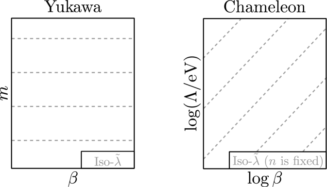
with $\tilde{\lambda}^{2}=\tilde{\lambda}^{2}_{\mathrm{Y}}=1/m^{2}L_{0}^{2}=(\lambda/L_{0})^{2}$ for the Yukawa model and $\tilde{\lambda}^{2}=\tilde{\lambda}^{2}_{\mathrm{C}}=(n+1)/m^{2}(\rho_{0})L_{0}^{2}$ for the chameleon model. Figure 1 depicts the dependence of $\tilde{\lambda}$ on the model parameters.

Hence $\phi_{0}$ is a function of the model parameters $(C,p,\beta)$ and of the properties of the system at hand through the free parameter $\rho_{0}$, but it does not depend on $L_{0}$. This non-dimensionalization procedure allows for a more efficient numerical exploration of these parameter spaces and lets us study a large variety of physical systems — in particular those of Table 1.

Our goal is to evaluate the effect of the smoothing of the matter distribution on a typical scale $L_{0}$ on the field distribution as well as its energy and pressure. To that purpose, we define the average of any scalar quantity $X({\bf x})$ on the scale $s$ as

with $W_{\!s}$ a window function of typical width $s$.

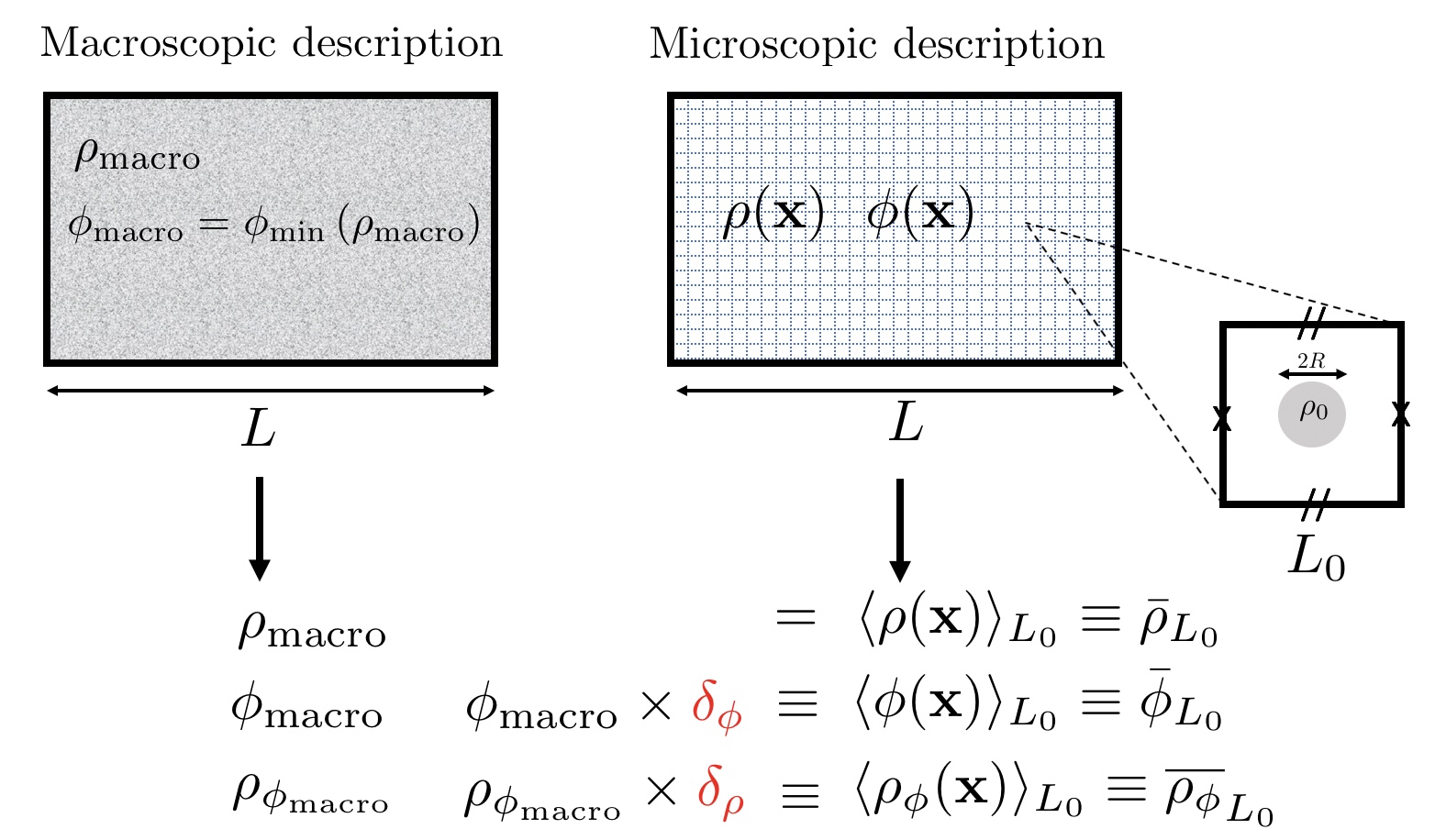
Now, we make the simplifying assumptions summarized on Fig. 2 following the formalism by Refs. Sanghai:2015wia ; Sanghai:2016ucv ; Sanghai:2017yyn ; Sikora:2018imr ; Briddon:2024ftz . We consider a medium that is modeled with two descriptions:

1. 1.

   Macroscopic. On a large scales, the medium is homogeneous and continuous so that it can be described as a fluid with constant density $\rho_{\rm macro}$. For a static configuration the scalar field has thus the constant value

   $$\phi_{\rm macro}\equiv\phi_{\min}(\rho_{\rm macro})\,,$$

   (9)

   that is indeed not necessarily strictly positive; see Eq. (6).

2. 2.

   Microscopic. On the local scale, the fluid is described by spherical particles of radius $R$ with constant mass density $\rho_{0}$ in vacuum. For simplicity, we assume that these particles occupy the centers of a regular lattice of size $L_{0}$. For each representative elementary volume, the local matter distribution is thus given by $\rho(\mathbf{x})\equiv 0$ if $\mathbf{x}\notin\mathcal{B}(R)$ and $\rho(\mathbf{x})=\rho_{0}$ otherwise, with $\mathcal{B}(R)$ the ball of radius $R$ centered on $\mathbf{0}$. The field distribution $\phi(\bf x)$ is then solution of the KG equation with this source term and periodic boundary conditions. To be more specific, we consider the domain of integration to $\Omega$ a cube of side length $L_{0}$ and boundary $\Gamma$. We also define $\tilde{\Omega}$ the cube of unit side length with boundary $\tilde{\Gamma}$ .

The descriptions on these two scales are related by the fact that we shall impose ${\rho_{\rm macro}=\langle\rho({\bf x})\rangle_{L_{0}}\equiv\bar{\rho}_{L_{0}}}$, hence for homogeneous distribution on ${\cal B}$

which for a sphere imposes

This expresses the fact that the fluid mass density $\rho_{\rm macro}$ is related to the mass density and size of the particles that compose it and their mean separation.

Hence, the microscopic description of matter fixes $\rho_{0}$ and $R$ while the macroscopic description fixes $L_{0}$. Then, $\phi_{0}$ is algebraically determined by Eq. (6) while $\phi_{\rm macro}$ is given by Eq. (9). The typical values of the physical parameters for the systems of interest are gathered in Table 1.

In order to discuss the effect of the coarse graining, we shall compare the averages of the field distribution and energy density to the ones of the large-scale homogeneous description with $\rho_{\rm macro}$. We thus define the two quantities $\delta_{\phi}$ and $\delta_{\rho}$ by

with $\phi_{\rm macro}$ given by Eq. (9) and $\rho_{\phi_{\rm macro}}=V(\phi_{\rm macro})$ the energy density of the smooth field distribution. We use the similar quantity $\delta_{P}$ for the isotropic pressure.

In a quadratic scalar field theory such as the Yukawa theory, i.e. with a linear KG equation, one expects $\delta_{\phi}=1$ while $\delta_{\rho}\not=1$ and $\delta_{P}\not=1$ whatever the theory since the energy density is a quadratic function of the field. Indeed non-linear scalar field theories such as the chameleon model will lead to $\delta_{\phi}\not=1$. The goal of the two following sections is to estimate the magnitude of these three quantities.

First, before even having to solve the KG equation, it is clear that one expects from linearity that the averaging procedure shall commute with the equation. Indeed, from the divergence theorem, the l.h.s. of Eq. (7) gives

the last equality following from the periodic boundary conditions [see Eq. (37)]. It follows that

i.e., $\langle\tilde{\phi}\rangle_{1}=-\langle\tilde{\rho}\rangle_{1}$, a relation that interestingly does not depend on the parameter $\tilde{\lambda}^{2}$. The average of the field distribution is thus given by $\bar{\phi}_{L_{0}}\equiv\langle\phi\rangle_{L_{0}}=$ $\phi_{0}\langle\tilde{\phi}\rangle_{1}=$ $-\phi_{0}\langle\tilde{\rho}\rangle_{1}=-\phi_{0}\rho_{\rm macro}/\rho_{0}$, so that, from Eqs. (4) and (9),

as anticipated.

To be more quantitative and compare to our numerical integration of the KG equation, let us remind that in the Yukawa theory, the linear differential operator ${(\Delta-1/\lambda^{2})}$ has a free-space Green function

Hence the field generated by a point particle source, i.e. with $\rho({\bf x})=M\delta_{\rm D}({\bf x})$ is

As detailed in Appendix D, the field distribution generated by a sphere of radius $R$ and constant density $\rho_{0}$ is

respectively oustside and inside the sphere, with ${M=4\pi\rho_{0}R^{3}/3}$ and

It is easily checked that this expression is indeed smooth in $r=R$ and that the usual Newtonian expressions are obtained in the limit $\lambda\rightarrow+\infty$.

These expressions allow us to qualitatively discuss the effect of the mass distribution, i.e. the choice of $(R,\rho_{0})$ while $M$ is kept identical. First, inside the sphere, Eq. (14) can be rewritten as

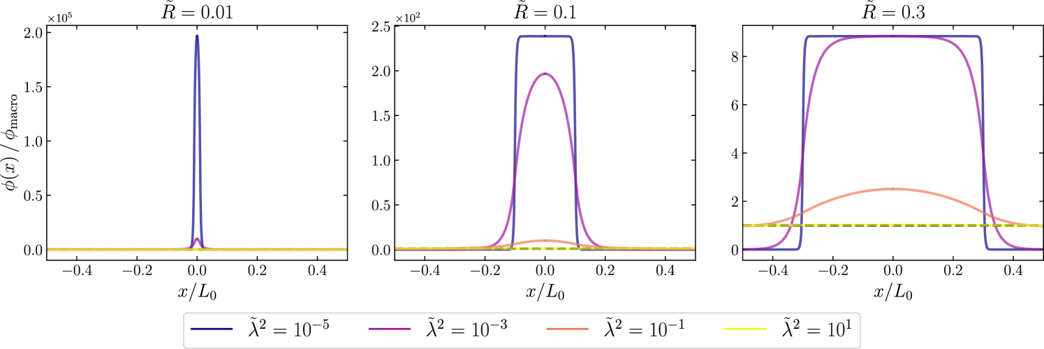
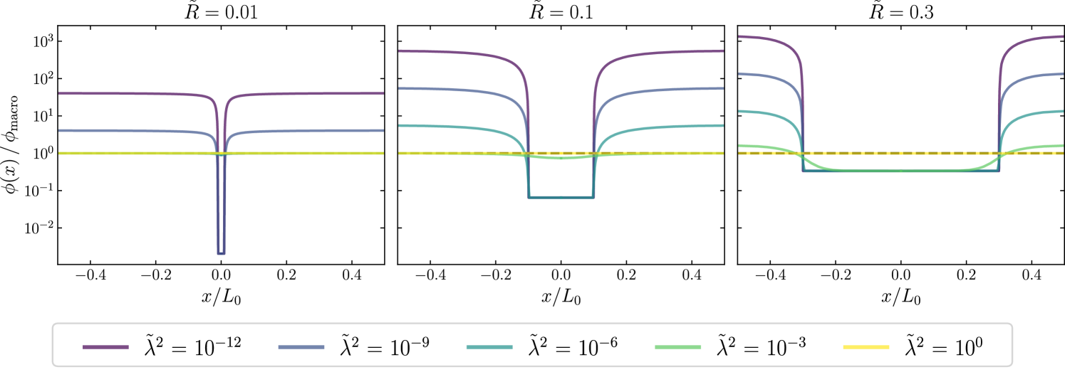
showing that the field is driven exponentially close to $\phi_{\rm min}$ if $R/\lambda$ is large enough, i.e., if the field’s Compton wavelength to be much smaller than $R$. Typically $|\phi(0)/\phi_{\rm min}-1|<1\%$ for $R/\lambda\gtrsim 6.6$. Then, outside the the sphere, the field relaxes to $0$ but its amplitude is rescaled by the factor $\Phi(R/\lambda)$ compared to a point particle with same mass. All these features are numerically illustrated on Fig. 3 even though they take into account the periodic boundary conditions necessary to represent the infinite lattice. All the field profiles depicted on Fig. 3 have different $(R,\rho_{0})$ with same total mass, i.e. same $\rho_{\rm macro}$. It is easily checked that while the field distributions $\phi({\bf x})$ depend on both $(R,\rho_{0})$ and the parameter $(\lambda,\beta)$, they all share the same mean value $\bar{\phi}_{L_{0}}$, i.e. $\delta_{\phi}=1$ for all models and all parameters enjoying the same $\bar{\rho}_{L_{0}}$.

Since the stress energy tensor (29) is quadratic in the scalar field, all these field profiles sharing the same mean value (see Fig. 3) have different energy densities. Let us evaluate how the coarse grained energy depend on the small-scale distribution of matter, i.e., on the parameters $(R,\rho_{0})$ with same $\rho_{0}R^{3}$. The general expression (33) of the mean energy density of the scalar field, $\overline{\rho_{\phi}}_{L_{0}}$ reduces to

for a Yukawa model (since $p=2$). This expression has been interpreted as a binding energy in Ref. Fleury:2016tsz . For a sphere, if one approximates the field by the spherically symmetric solution (14) which indeed neglects the periodic boundary conditions, one can get the approximation

with $\tilde{\phi}(\tilde{r})\simeq-\left[1-\hbox{e}^{-\tilde{R}/\tilde{\lambda}}(\tilde{R}/\tilde{\lambda}+1)\frac{\sinh(\tilde{r}/\tilde{\lambda})}{\tilde{r}/\tilde{\lambda}}\right]$ and $\tilde{\rho}=1$ on ${\cal B}(R)$. The $\simeq$ symbol is used to recall we neglect the boundary conditions imposed by the large-scale structure. Hence,

It follows that in the limit of small $\tilde{\lambda}$,

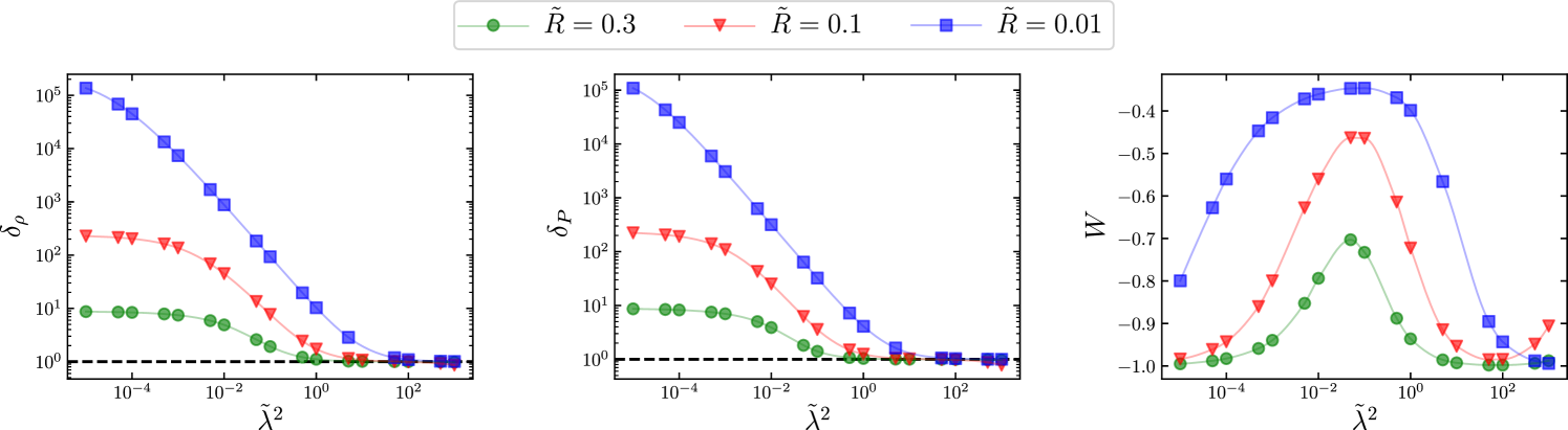
which explains that $\delta_{\rho}$ reaches a plateau with an amplitude that scales as $\tilde{R}^{-3}$, as obtained numerically on Fig. 4. At large $\tilde{\lambda}$, $\delta_{\rho}\simeq 1$, which can be explained by the fact that the field is less screened. The deviation from $\delta_{\rho}=1$ increases with the clumpiness of matter, i.e. when $\tilde{R}$ decreases which is indeed intuitive since when $4\pi\tilde{R}^{3}/3\rightarrow 1$, $\rho_{0}\rightarrow\rho_{\rm macro}$ and the sphere fills the whole domain. This analytic approximation has been checked to give the exact value of the plateau of Fig. 4 in the limit $\tilde{\lambda}\ll 1$.

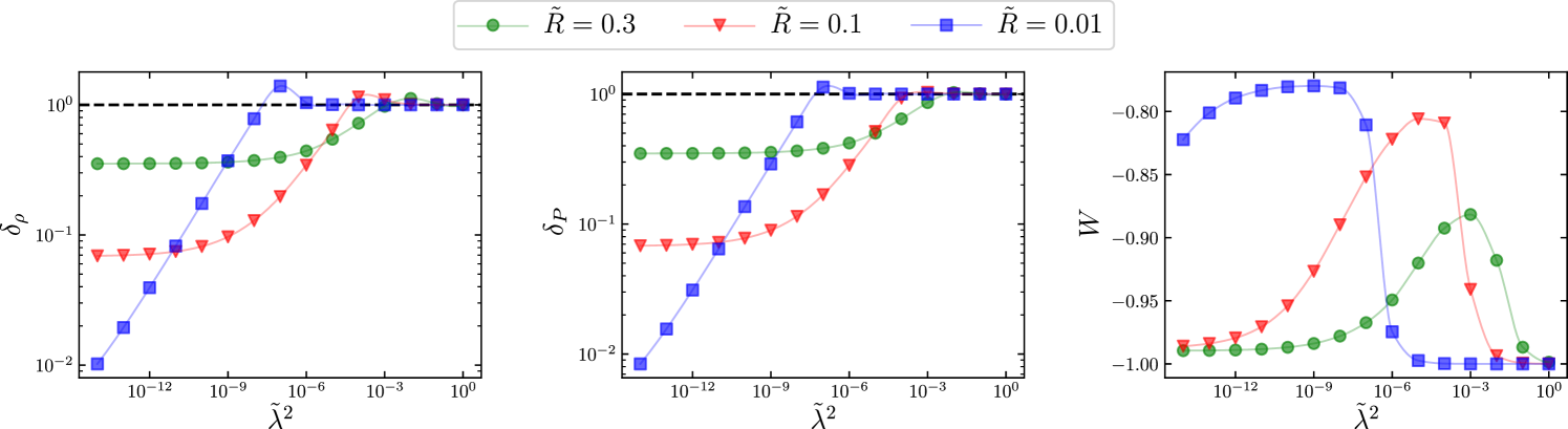
This analysis can be extended to compute the coarse grained isotropic pressure. The results are gathered on Fig. 4 that show a similar behavior for $\delta_{P}$. We also consider the equation of state of the scalar field. On the macroscopic scales $P_{\phi}(\phi_{\rm macro})=-\rho_{\phi}(\phi_{\rm macro})$ so that $w_{\rm macro}=-1$, while the equation of state of the coarse-grained distribution is

In order to interpret these numerical results, notice that for large $\tilde{\lambda}$ the matter source remains unscreened. The field is almost not affected by the matter on the scale $\tilde{R}$ so that it can be treated perturbatively. Hence one concludes that both $\delta_{\rho}$ and $\delta_{P}$ tend toward 1 and hence $W=-1$. For small $\tilde{\lambda}$, the matter sphere are screened so that the field reaches its two minima in the whole sphere and in the inter-sphere space — but in a small layer $\Delta R$. It follows that the contribution of $(\nabla\phi)^{2}$ in the field pressure (32) becomes negligible since $\epsilon\equiv\Delta R/R\ll 1$. Hence the expressions (31-32) lead to the conclusion that $W=-1$, as confirmed by the numerical integrations on Fig. 4.

These results drive a series of remarks.

1. 1.

   In the cosmological context, the energy density and pressure of the scalar field smoothed on cosmological scales shall enter the Friedmann equation. This effect has been investigated in Ref. Briddon:2024ftz in their “post-Newtonian approach to cosmological modeling”, with which we share the same description of the microscopic distribution of matter. They concluded that the Friedmann equation shall take he generic form

   $$H^{2}=\frac{8\pi G}{3}\left[\Big{\langle}\rho({\bf x},t)\Big{\rangle}+\Big{\langle}\frac{1}{2}\dot{\phi}({\bf x},t)+V[\phi({\bf x},t)]\Big{\rangle}\right]$$

   which includes the fluctuations of the field on $\dot{\phi}$ but neglects the $\nabla\phi$ contribution to the scalar field energy density (31). This is indeed a good approximation when the post-Newtonian formalism can be applied, i.e., gravity is described by a metric and that it does not involve any characteristic scale will ; blanchet on the size of the system studied. in the present case, this corresponds to the limit $\tilde{\lambda}\gg 1$, a regime in which we fully recover the conclusions of Ref. Briddon:2024ftz . This is indeed not the case otherwise, as shown on Fig. 4. The $\tilde{\lambda}\leq 1$ regime is indeed much more subtle to model. If we boldly assume that the Friedmann equations take the form – which indeed is probably not the case,

   	$\displaystyle H^{2}$	$\displaystyle=$	$\displaystyle\frac{8\pi G}{3}\left(\overline{\rho}+{\overline{\rho_{\phi}}}\right)$
   	$\displaystyle\frac{\ddot{a}}{a}$	$\displaystyle=$	$\displaystyle-\frac{4\pi G}{3}\left(\overline{\rho}+3\overline{P}+{\overline{\rho_{\phi}}}+3{\overline{P_{\phi}}}\right)$

   as long as it is described in the Einstein frame, which is indeed not the observational frame — see point 2 below – then the computation of the full energy density is required, with the gradient terms included.

   As already emphasized ${\overline{\rho_{\phi}}}\not=\rho_{\phi}(\phi_{\rm macro})$ and Fig. 4 let us expect that they can significantly differ. Indeed, in our numerics are restricted to a static configuration and we not solve the KG equation on a FL background spacetime. Still, we can speculate that (1) in perturbation theory this is a lower order effect and the cosmological dynamics is well described by the usual approach relying on a FL solution as already concluded in Ref. Briddon:2024ftz ; (2) in the regime $\tilde{\lambda}\gg 1$, studied in Ref. Briddon:2024ftz , it is a good approximation to consider the smooth value of the field to infer the cosmological dynamics and (3) in the regime $\tilde{\lambda}\ll 1$ while, $\delta_{\rho}$ and $\delta_{P}$ become large, we expect the cosmological dynamics to significantly differ from the one inferred under the approximation of a smooth scalar field, even if, quite surprizingly, the equation of state seems not to be modified deep in this regime.

   Our present analysis does not allow us to draw definite conclusions, but it signals that the cosmological conclusions for dark energy models coupled to matter shall be revisited with care, maybe by extending the analysis of Ref. Briddon:2024ftz or our present work.

2. 2.

   An additional point is worth emphasizing. So far, we have used the Einstein-frame description but observations shall be analyzed in the Jordan frame Esposito-Farese:2000pbo ; Uzan:2006mf . It follows that

   $$a_{\rm JF}=A(\phi)a_{\rm EF}\,$$

   and

   $$\rho_{\rm JF}=A^{4}(\phi)\rho_{\rm EF},\,P_{\rm JF}=A^{4}(\phi)P_{\rm EF}$$

   respectively for the scale factor, energy density and pressure in both frames. Since the coupling $A(\phi)$ is not linear, it is then obvious that

   $$\langle A(\phi)\rangle a_{\rm EF}\not=A(\phi_{\rm macro})a_{\rm EF}$$

   and similarly

   $$\langle\rho_{\rm JF}\rangle=\langle A^{4}(\phi)\rho_{\rm EF}\rangle\not=A^{4}(\phi_{\rm macro})\langle\rho_{\rm EF}\rangle\,.$$

   Indeed, these effects are usually taken into account at linear order in cosmological perturbations but can become large when the clumpiness of matter becomes important.

3. 3.

   As seen on Fig. 4, the equation of state remains larger than $-1$, $W\geq-1$, and is still driving an acceleration since $W<-1/3$. Hence, one shall expect the effect of the clustering to lead to a milder acceleration. Even in the case of a Yukawa model with a large mass compared to the Hubble parameter, so that the macroscopic dynamics leads to a pure cosmological constant since the field is stuck at the minimum of its potential, one expects $W>-1$. Indeed our analysis is restricted to a static distribution so that it has to be extended to derived the proper cosmological effects. But it shows the effect is present.

4. 4.

   It follows that extra-care is needed for the interpretation of extended quintessence models even if the KG equation is linear and $\bar{\phi}=\phi_{\rm macro}$ since the clumpiness of matter will be more important at small redshifts and hence modify the late time prediction of the observables. This also the case in models Pitrou:2023swx ; Uzan:2023dsk in which the scalar field coupled simply to a dark matter component to avoid variations of fundamental constants Uzan:2024ded .

Hence, this example, even if not realistic and restricted to a static matter distribution, shows that the averaging of the scalar can bias the interpretation of scalar field model when coupled to matter.

Let us now consider a non-linear KG equation as arises in chameleon models. Unfortunately, such a scenario cannot be fully addressed analytically. Still, repeating step by step the argument of § III.1, one easily shows that

from which one concludes that, thanks to Eqs. (4) and (6)

This shows that the field distribution with different microscopic geometries with constant $\bar{\rho}_{L_{0}}$ will still share some common averaged quantities, but they will indeed have different mean values of $\phi$ so that $\delta_{\phi}\not=1$. This generically implies, a fortiori, that the field energy density will have very different mean values.

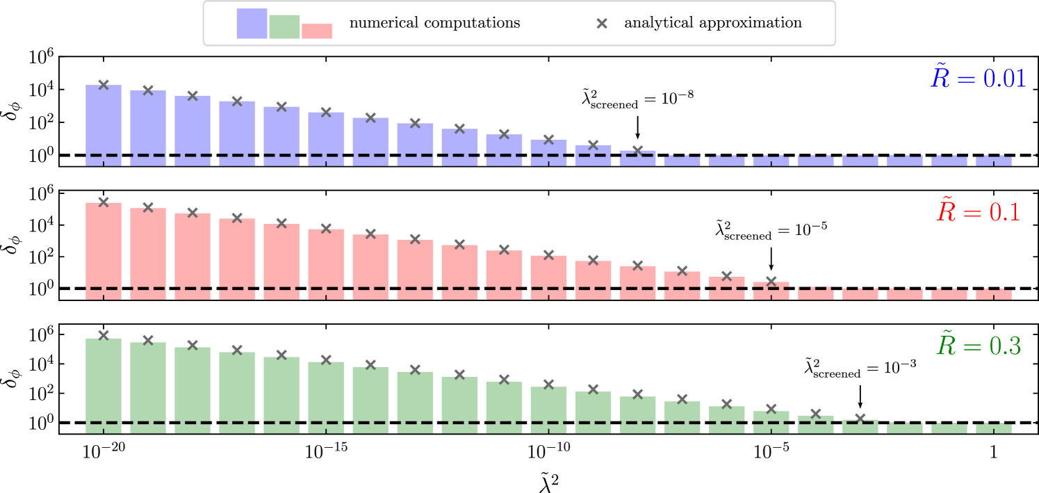
Figure 5 depicts several chameleon field profiles normalized by $\phi_{\mathrm{macro}}$ evaluated along one of the principal axis of the cube. Some of the comments made on the Yukawa field profiles (see Fig. 3) still apply to the present case. In particular, the limits $\tilde{\lambda}\to 0^{+}$ and $\tilde{\lambda}\to+\infty$ have similar effects on the chameleon field dynamics: in the former limit, the field reaches the minimum of its effective potential inside the sphere; whereas in the latter limit, the field relaxes to the constant $\phi_{\mathrm{macro}}$ everywhere. The main difference with respect to the Yukawa model — as already emphasized  — is that $\delta_{\phi}\neq 1$ in the so-called screened regime. This point is not necessarily obvious from Fig. 5, which is why we compute $\delta_{\phi}$ for three distinct geometries and for a wide range of parameters $\tilde{\lambda}$ in Fig. 6. Two comments are in order from theses numerical results:

1. 1.

   When the system is unscreened on the smoothing scale $L_{0}$, which is typically the case when $\tilde{\lambda}\gtrsim 1$, one recovers $\delta_{\phi}=1$ despite the non-linerarities.

2. 2.

   In the screened regime however, i.e. for sufficiently small values of $\tilde{\lambda}$, $\delta_{\phi}$ departs from unity, reaching values larger than $10^{5}$.

In the latter case, i.e. when the matter sphere is screened, we can even derive an analytical approximation of $\delta_{\phi}$. Following the steps detailed in Appendix E, we get

with

This analytical approximation is depicted by gray crosses and compared against the numerical computations in Fig. 6. The two approaches — analytical and numerical — agree remarkably well. Consequently, it seems legitimate to make use of Eqs. (21) and (22) to extrapolate values of $\delta_{\phi}$ for even smaller parameters $\tilde{\lambda}$. Moreover, Eq. (21) also turns out to be also useful for approximating $\tilde{\lambda}_{\mathrm{screened}}$, by checking when Eq. (21) produces $\delta_{\phi}\simeq 1$ (see gray crosses on Fig. 6). Here, $\tilde{\lambda}_{\mathrm{screened}}$ refers to the specific value of $\tilde{\lambda}$ where the transition between the two regimes occurs.

Note that a similar analysis has been performed in Ref. Briddon:2024ftz and that our field profiles from Fig. 5 have the same generic form that those presented in their Fig. 5 even though we do not use the same boundary conditions. Still, deep in the screened regime, the two computation led to consistent conclusions since the parameter $\alpha$ in Eqs. (48-29) of Ref. Briddon:2024ftz introduced in the averaged Friedmann equations (neglecting the gradient term in the energy density since it differs from 0 only in a thin shell) coincides with our ${\rm Vol}(\tilde{\Omega})=4\pi\tilde{R}^{3}/3$. The present work gives however a precise, numerical and analytical, value on $\delta_{\phi}$, i.e., on how the small scale structure affects the mean value of the scalar field.

Figure 7 gives the consequences of the fluid quantities and the equation of state. As for the field distribution, the consequences depend strongly on the screening.

In the unscreened regime, both $\delta_{\rho}$ and $\delta_{P}$ tend to unity so that $W=-1$. Interestingly this is also the case in the screened regime, for the same reason as for the Yukawa case: the field has strong variations between the inside and outside of the sphere but it is almost constant everywhere but on a thin shell of relative width $\epsilon$. Hence its gradient is almost zero everywhere and the local equation of state is equal to $-1$ almost everywhere.

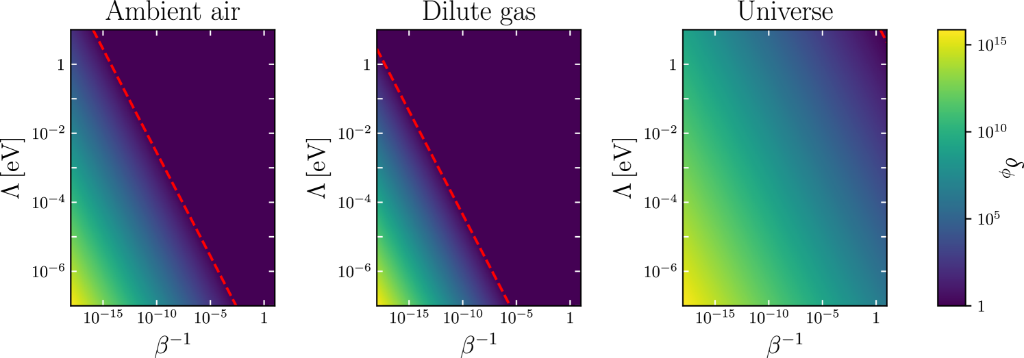
Then, from Fig. 8, we see that for typical values found in Table 1, galaxies are not screened, i.e. at late time the homogenous approximation used to draw cosmological consequences may not be a good. Hence, the field may not be following the minimum of its effective potential $V_{\rm eff}$ with $\rho=\rho_{\rm macro}$, and the effects on the cosmological dynamics may be strongly modified. Still the equation of state is reduced but less sharply than for the Yukawa case.

References

- (1) G. F. R. Ellis “Relativistic cosmology” in General Relativity and Cosmology, Enrico Fermi Summer School Course XLVII ed R. K. Sachs (New York:Academic, 1971) p. 104-182.
- (2) G. F. R. Ellis, “Relativistic Cosmology: Its Nature, Aims and Problems”, Fundam. Theor. Phys. 9, 215-288 (1984)
- (3) G. F. R. Ellis and W. Stoeger, “The ’fitting problem’ in cosmology”, Class. Quant. Grav. 4, 1697-1729 (1987)
- (4) G. F. R. Ellis and T. Buchert, “The Universe seen at different scales”, Phys. Lett. A 347, 38-46 (2005) [arXiv:gr-qc/0506106 [gr-qc]].
- (5) C. Clarkson, G. Ellis, J. Larena and O. Umeh, “Does the growth of structure affect our dynamical models of the universe? The averaging, backreaction and fitting problems in cosmology”, Rept. Prog. Phys. 74, 112901 (2011) [arXiv:1109.2314 [astro-ph.CO]].
- (6) T. Buchert, “On average properties of inhomogeneous fluids in general relativity. 1. Dust cosmologies”, Gen. Rel. Grav. 32, 105-125 (2000) [arXiv:gr-qc/9906015 [gr-qc]].
- (7) T. Buchert, “On average properties of inhomogeneous fluids in general relativity: Perfect fluid cosmologies”, Gen. Rel. Grav. 33, 1381-1405 (2001) [arXiv:gr-qc/0102049 [gr-qc]].
- (8) R. M. Zalaletdinov, “Averaging problem in general relativity, macroscopic gravity and using Einstein’s equations in cosmology”, Bull. Astron. Soc. India 25, 401-416 (1997) [arXiv:gr-qc/9703016 [gr-qc]].
- (9) R. Zalaletdinov, “The Averaging Problem in Cosmology and Macroscopic Gravity”, Int. J. Mod. Phys. A 23, 1173-1181 (2008) [arXiv:0801.3256 [gr-qc]].
- (10) A. Paranjape and T. P. Singh, “Structure Formation, Backreaction and Weak Gravitational Fields”, JCAP 03, 023 (2008) [arXiv:0801.1546 [astro-ph]].
- (11) T. Buchert and M. Carfora, “Regional averaging and scaling in relativistic cosmology”, Class. Quant. Grav. 19, 6109-6145 (2002) [arXiv:gr-qc/0210037 [gr-qc]].
- (12) E. A. Calzetta, B. L. Hu and F. D. Mazzitelli, “Coarse grained effective action and renormalization group theory in semiclassical gravity and cosmology”, Phys. Rept. 352, 459-520 (2001) [arXiv:hep-th/0102199 [hep-th]].
- (13) M. Carfora and K. Piotrkowska, “A Renormalization group approach to relativistic cosmology”, Phys. Rev. D 52, 4393-4424 (1995) [arXiv:gr-qc/9502021 [gr-qc]].
- (14) T. Futamase, “Averaging of a locally inhomogeneous realistic universe”, Phys. Rev. D 53, 681-689 (1996)
- (15) J. P. Boersma, “Averaging in cosmology”, Phys. Rev. D 57, 798-810 (1998) [arXiv:gr-qc/9711057 [gr-qc]].
- (16) W. R. Stoeger, S.J., A. Helmi and D. F. Torres, “Averaging Einstein’s equations: The Linearized case”, Int. J. Mod. Phys. D 16, 1001-1026 (2007) [arXiv:gr-qc/9904020 [gr-qc]].
- (17) P. Fleury, H. Dupuy and J. P. Uzan, “Interpretation of the Hubble diagram in a nonhomogeneous universe”, Phys. Rev. D 87, no.12, 123526 (2013) [arXiv:1302.5308 [astro-ph.CO]].
- (18) P. Fleury, H. Dupuy and J. P. Uzan, “Can all cosmological observations be accurately interpreted with a unique geometry?”, Phys. Rev. Lett. 111, 091302 (2013) [arXiv:1304.7791 [astro-ph.CO]].
- (19) I. Ben-Dayan, M. Gasperini, G. Marozzi, F. Nugier and G. Veneziano, “Do stochastic inhomogeneities affect dark-energy precision measurements?”, Phys. Rev. Lett. 110, no.2, 021301 (2013) [arXiv:1207.1286 [astro-ph.CO]].
- (20) Y. B. Zel’dovich, Sov. Astron. Lett. 8, 13 (1964); V. M. Dashevskii and Y. B. Zel’dovich, Sov. Astronom. 8, 854 (1965); J. E. Gunn, Astrophys. J. 150, 737 (1967); R. Kantowski, Astrophys. J. 155, 89 (1969); C. Dyer and R. Roeder, Astrophys. J. 174, L115 (1972); S. Weinberg, Astrophys. J. Lett. 208, L1 (1976); D. E. Holz and R. M. Wald, Phys. Rev. D 58, 063501 (1998); K. Bolejko and P. G. Ferreira, JCAP 5, 003 (2012).
- (21) C. Clarkson, G. F. R. Ellis, A. Faltenbacher, R. Maartens, O. Umeh and J. P. Uzan, “(Mis-)Interpreting supernovae observations in a lumpy universe”, Mon. Not. Roy. Astron. Soc. 426, 1121-1136 (2012) [arXiv:1109.2484 [astro-ph.CO]].
- (22) P. Fleury, J. Larena and J. P. Uzan, “The theory of stochastic cosmological lensing”, JCAP 11, 022 (2015) [arXiv:1508.07903 [gr-qc]].
- (23) P. Fleury, J. Larena and J. P. Uzan, “Weak gravitational lensing of finite beams”, Phys. Rev. Lett. 119, no.19, 191101 (2017) [arXiv:1706.09383 [gr-qc]].
- (24) P. Fleury, J. Larena and J. P. Uzan, “Cosmic convergence and shear with extended sources”, Phys. Rev. D 99, no.2, 023525 (2019) [arXiv:1809.03919 [astro-ph.CO]].
- (25) P. G. Ferreira and M. Joyce, “Structure formation with a selftuning scalar field”, Phys. Rev. Lett. 79, 4740-4743 (1997) [arXiv:astro-ph/9707286 [astro-ph]].
- (26) P. Creminelli, G. D’Amico, J. Norena and F. Vernizzi, “The Effective Theory of Quintessence: the w-1 Side Unveiled”, JCAP 02, 018 (2009) [arXiv:0811.0827 [astro-ph]].
- (27) P. Creminelli, G. D’Amico, J. Norena, L. Senatore and F. Vernizzi, “Spherical collapse in quintessence models with zero speed of sound”, JCAP 03, 027 (2010) [arXiv:0911.2701 [astro-ph.CO]].
- (28) J. P. Uzan, “Cosmological scaling solutions of nonminimally coupled scalar fields”, Phys. Rev. D 59, 123510 (1999) [arXiv:gr-qc/9903004 [gr-qc]].
- (29) H. Lévy and J. P. Uzan, “Testing screened scalar-tensor theories of gravity with atomic clocks”, Phys. Rev. D 111, no.6, 064012 (2025) [arXiv:2410.17292 [gr-qc]].
- (30) P. Brax, C. van de Bruck, A. C. Davis, J. Khoury and A. Weltman, “Detecting dark energy in orbit: The cosmological chameleon”, Phys. Rev. D 70, 123518 (2004) [arXiv:astro-ph/0408415 [astro-ph]].
- (31) P. Brax, C. van de Bruck, A. C. Davis, J. Khoury and A. Weltman, “Chameleon dark energy”, AIP Conf. Proc. 736, no.1, 105-110 (2004) [arXiv:astro-ph/0410103 [astro-ph]].
- (32) D. F. Mota and D. J. Shaw, “Evading Equivalence Principle Violations, Cosmological and other Experimental Constraints in Scalar Field Theories with a Strong Coupling to Matter,” Phys. Rev. D 75 (2007), 063501 [arXiv:hep-ph/0608078 [hep-ph]].
- (33) D. F. Mota and D. J. Shaw, “Strongly coupled chameleon fields: New horizons in scalar field theory,” Phys. Rev. Lett. 97 (2006), 151102 [arXiv:hep-ph/0606204 [hep-ph]].
- (34) H. Lévy, J. Bergé and J. P. Uzan, “Solving nonlinear Klein–Gordon equations on unbounded domains via the finite element method”, Phys. Rev. D 106, no.12, 124021 (2022) [arXiv:2209.07226 [gr-qc]].
- (35) H. Lévy, “Towards well-posed and versatile numerical solutions of scalar-tensor theories of gravity with screening mechanisms : applications at sub-Solar system scales”, tel-04789073 (PhD thesis, 2024).
- (36) H. Lévy, J. Bergé and J. P. Uzan, “What to expect from scalar-tensor space geodesy”, Phys. Rev. D 109, no.8, 084009 (2024) [arXiv:2310.03769 [gr-qc]].
- (37) J. Khoury and A. Weltman, “Chameleon cosmology”, Phys. Rev. D 69, 044026 (2004) [arXiv:astro-ph/0309411 [astro-ph]].
- (38) J. Khoury and A. Weltman, “Chameleon fields: Awaiting surprises for tests of gravity in space”, Phys. Rev. Lett. 93, 171104 (2004) [arXiv:astro-ph/0309300 [astro-ph]].
- (39) K. Hinterbichler and J. Khoury, “Symmetron Fields: Screening Long-Range Forces Through Local Symmetry Restoration”, Phys. Rev. Lett. 104, 231301 (2010) [arXiv:1001.4525 [hep-th]].
- (40) V. A. A. Sanghai and T. Clifton, “Post-Newtonian Cosmological Modelling”, Phys. Rev. D 91, 103532 (2015) [erratum: Phys. Rev. D 93, no.8, 089903 (2016)] [arXiv:1503.08747 [gr-qc]].
- (41) V. A. A. Sanghai and T. Clifton, “Cosmological backreaction in the presence of radiation and a cosmological constant”, Phys. Rev. D 94, no.2, 023505 (2016) [arXiv:1604.06345 [gr-qc]].
- (42) V. A. A. Sanghai, P. Fleury and T. Clifton, “Ray tracing and Hubble diagrams in post-Newtonian cosmology”, JCAP 07, 028 (2017) [arXiv:1705.02328 [astro-ph.CO]].
- (43) S. Sikora and K. Głód, “Perturbatively constructed cosmological model with periodically distributed dust inhomogeneities”, Phys. Rev. D 99, no.8, 083521 (2019) [arXiv:1811.06836 [gr-qc]].
- (44) C. Briddon, T. Clifton and P. Fleury, “Emergent cosmological expansion in scalar–tensor theories of gravity”, Class. Quant. Grav. 42, no.1, 015013 (2025) [arXiv:2406.01397 [gr-qc]].
- (45) P. Fleury, “Cosmic backreaction and Gauss’s law”, Phys. Rev. D 95, no.12, 124009 (2017) [arXiv:1609.03724 [gr-qc]].
- (46) C.M. Will, Theory and Experiment in Gravitational Physics (Cambridge University Press, Cambridge; New York, 1993).
- (47) L. Blanchet, “Gravitational radiation from post-Newtonian sources and inspiralling compact binaries”, Living Rev. Relativ 9:4 (2006) [https://doi.org/10.12942/lrr-2006-4. grqc/ 0202016].
- (48) C. Pitrou and J. P. Uzan, “Hubble Tension as a Window on the Gravitation of the Dark Matter Sector”, Phys. Rev. Lett. 132, no.19, 191001 (2024) [arXiv:2312.12493 [astro-ph.CO]].
- (49) J. P. Uzan and C. Pitrou, “Hubble tension as a window on the gravitation of the dark matter sector: Exploration of a family of models”, Phys. Rev. D 109, no.10, 103505 (2024) [arXiv:2312.12408 [astro-ph.CO]].
- (50) G. Esposito-Farese and D. Polarski, “Scalar tensor gravity in an accelerating universe”, Phys. Rev. D 63, 063504 (2001) [arXiv:gr-qc/0009034 [gr-qc]].
- (51) J. P. Uzan, “The acceleration of the universe and the physics behind it”, Gen. Rel. Grav. 39, 307-342 (2007) [arXiv:astro-ph/0605313 [astro-ph]].
- (52) J. P. Uzan, “Fundamental constants: from measurement to the universe, a window on gravitation and cosmology”, [arXiv:2410.07281 [astro-ph.CO]].
- (53) C. Burrage and J. Sakstein, “Tests of Chameleon Gravity”, Living Rev. Rel. 21, no.1, 1 (2018) [arXiv:1709.09071 [astro-ph.CO]].
- (54) M. Pernot-Borràs, J. Bergé, P. Brax and J. P. Uzan, “General study of chameleon fifth force in gravity space experiments”, Phys. Rev. D 100, no.8, 084006 (2019) [arXiv:1907.10546 [gr-qc]].
- (55) M. Pernot-Borràs, J. Bergé, P. Brax and J. P. Uzan, “Fifth force induced by a chameleon field on nested cylinders”, Phys. Rev. D 101, no.12, 124056 (2020) [arXiv:2004.08403 [gr-qc]].
- (56) M. Pernot-Borràs, J. Bergé, P. Brax, J. P. Uzan, G. Métris, M. Rodrigues and P. Touboul, “Constraints on chameleon gravity from the measurement of the electrostatic stiffness of the MICROSCOPE mission accelerometers”, Phys. Rev. D 103, no.6, 064070 (2021) [arXiv:2102.00023 [gr-qc]].
- (57) C. Robert, “Fast evaluation of finite element weak forms using python tensor contraction packages”, Advances in Engineering Software 159, 103033 (2021)
- (58) M. Abramowitz, and I.A. Stegun, Handbook of Mathematical Functions with Formulas, Graphs, and Mathematical ables, (Dover Publications, New York, 1964).