Scattering expansion for localization in one dimension: From disordered wires to quantum walks
Abstract
We present a perturbative approach to disordered systems in one spatial dimension that accesses the full range of phase disorder and clarifies the connection between localization and phase information. We consider a long chain of identically disordered scatterers and expand in the reflection strength of any individual scatterer. We apply this expansion to several examples, including the Anderson model, a general class of periodic-on-average-random potentials, and a two-component discrete-time quantum walk, showing analytically in the latter case that the localization length can depend non-monotonically on the strength of phase disorder (whereas expanding in weak disorder yields monotonic decrease). More generally, we obtain to all orders in the expansion a particular non-separable form for the joint probability distribution of the transmission coefficient logarithm and reflection phase. Furthermore, we show that for weak local reflection strength, a version of the scaling theory of localization holds: the joint distribution is determined by just three parameters.
I Introduction
The localization of waves by disorder (Anderson localization) is a topic of enduring interest due to the wide range of settings in which it occurs, including electron transport, classical optics, acoustics, and Bose-Einstein condensates [1]. Progress in the general theory of localization, independent of model details or of physical realization, can have similarly broad implications. Another setting for localization, of recent interest as a potential quantum computing platform [2, 3, 4], is the quantum walk [5, 6, 7], which is a quantum version of the classical random walk. Localization has been demonstrated in quantum walks both experimentally and theoretically [8, 9, 10, 11, 12, 13, 14, 15, 16, 17, 18, 19] and could impact quantum computing proposals even in the idealized limit of no decoherence [13, 14, 20, 21].
A distinctive feature of localization in quantum walks is the prominent role of phase disorder. Modern experimental platforms allow a high degree of control over a spatially varying phase which can be disordered [8, 9, 10, 11]. Localization in what is perhaps the simplest quantum walk, a discrete-time quantum walk (DTQW) in one spatial dimension, has been experimentally realized both for strong phase disorder [9] and for a controllable range of phase disorder from weak to strong [11]. However, existing analytical approaches seem to apply only in the limiting cases when phase disorder is either weak or strong [18, 19]. Furthermore, there are several phases that can appear in the quantum “coin” (see below) of a DTQW [22, *ChandrashekarErratum2010, 18], and a localization calculation that allows them all to be disordered simultaneously seems to be lacking in the literature.
A pillar of our general understanding of localization is the scaling theory initiated by Abrahams et al. in Ref. [24] in the context of electron transport. While localization may be characterized in several ways, including the absence of diffusion and the exponential decay of eigenstates, the scaling theory focuses on the suppression of the dimensionless conductance through a disordered sample (e.g., a cube of side length ). The conductance has some probability distribution over disorder realizations, and the scaling theory asserts that for sufficiently large , all dependence of the function on and on microscopic details may be absorbed into a small (i.e., at least not growing with ) number of parameters that obey scaling equations of the form (see, e.g, Refs. [25, 26]). The study of these scaling equations, and of the number of parameters needed in various cases, gives insight into disorder-driven phase transitions and has been a significant area of research in disordered systems.
In one spatial dimension, in which case localization is generally strongest, one can use a scattering setup [27] based on the Landauer formula for the conductance: , where is the transmission coefficient (we consider the case of a single scattering channel) of the sample 111To be precise, we are considering here the two-terminal conductance rather than the four-terminal conductance [106], where is the reflection coefficient of the sample; however, the distinction does not matter in the localized regime (in which ) that is our focus throughout. Also, we are ignoring spin degeneracy. In the rest of the paper, we set .. The typical transmission coefficient of a long sample of length decays exponentially: , which defines the localization length . In the transfer matrix approach, theorems for random matrices demonstrate that the probability distribution over disorder realizations [which by the Landauer formula is simply related to ] is Gaussian for large [29]. All dependence of on and on disorder thus reduces to two parameters (the mean and variance). A further reduction called single-parameter scaling (SPS), in which the two parameters reduce to one by an equation relating them, was originally obtained using an assumption of phase uniformity [27], but has since been shown to hold in certain limits even without this assumption [30, 31, 32].
In this paper, we present a perturbative approach to localization in one spatial dimension. Our scattering-based approach accesses the full range of phase disorder, clarifies the connection between localization and phase information more broadly, and applies to a general class of systems that includes DTQWs [33]. A central feature of our approach is the relation between the localization properties and the reflection phase of a disordered sample [27, 34, 35]. (This phase has been measured in a DTQW experiment [36].) We calculate the localization length and the probability distribution of the reflection phase, and we extend the scaling theory to include correlations between the reflection phase and the transmission coefficient. For a Letter version of this paper, see Ref. [37].
We now summarize our approach and results in more detail. We consider a disordered sample consisting of many single-channel scatterers that are independently and identically disordered, and we expand in the magnitude of the reflection amplitude of any individual scatterer 222As we comment on in the main body of this paper and in Appendix B, some of the results of our expansion at leading order were obtained in an equivalent form by Schrader et al. in Ref. [32] (see also Ref. [53]). Also, in the context of light propagation in disordered metamaterials, a similar expansion called the weak scattering approximation (WSA) was done in Refs. [93, 94] (see [95] for a review); however, the WSA has an uncontrolled aspect that is not present in our work (see Appendix C).. Our first main result is the expansion of the inverse localization length. We construct this expansion recursively and show that all orders depend only on local averages (that is, disorder averages over any single site). We obtain a similar expansion of the probability distribution of the reflection phase (finding that it is generally uniform only at the zeroth order), and indeed use this expansion in calculating the localization length.
We proceed to apply our first result to disordered wires and DTQWs. In the former case, we consider both the Anderson model and a broad class of periodic-on-average random systems (PARS), verifying that our results agree with and extend results from the literature. (For general background on PARS, see, e.g., Ref. [39] and references therein.) We then calculate the localization length analytically as a function of arbitrary phase disorder in a two-component DTQW in one dimension. We expect our calculation to apply to scattering setups [33] and beyond, and indeed we verify that our result interpolates between known results for weak and strong disorder that were calculated without reference to scattering [18, 19]. We find that the localization length can depend non-monotonically on the strength of phase disorder (similar to behavior seen numerically in Refs. [11, 18]) 333Non-monotonicity in disorder strength has been found previously, both analytically and numerically, in particular PARS problems [35, 83] (see Sec. III.3.2). Also, it has been shown that transmission through a disordered region can be non-monotonic in disorder strength when the incident wave is in an energy gap of the non-disordered system (see Ref. [107] and references therein); we do not consider this case.. Our expansion applies when the quantum “coin” is highly biased (see below), which is a regime of interest for optimizing quantum search [22, *ChandrashekarErratum2010]. Even if the coin is only moderately biased, we find favorable agreement with numerics using the first two non-vanishing orders of our expansion.
Our second main result concerns the joint probability distribution , where is the reflection phase of the disordered region. We use an ansatz to find that for large and to all orders in the scattering expansion, tends to a Gaussian function (of ) with mean, variance, and overall scale all depending on and all calculable order by order in terms of local averages. We further show that at the leading order in the local reflection strength, a version of the scaling theory applies: the joint distribution is determined by three parameters, which we may take to be the mean of and the mean and variance of . The latter two reach constant values for large system size ( in the notation used above).
Another contribution of this paper is to extend the perturbative derivation of SPS by Schrader et al. [32], while also explicitly connecting their result to a scattering setup. As we review in the main text, Ref. [32] demonstrates SPS in a general setting at the leading order in a small parameter. We point out that in a scattering setup, the local reflection strength is a valid choice for this parameter, which confirms (without assuming phase uniformity) the expectation in the literature that SPS should hold for weak local scattering [26]. We also extend the SPS relation to another order in the local reflection strength. (SPS cannot hold generally at the next order beyond, as Schrader et al. have shown that the Anderson model is a counter-example [32].) Note then that both SPS (for the distribution of ) and the three-parameter scaling that we find for the joint distribution are obtained in the same regime (weak local scattering).
We now make several comments about the scope of this paper. First, we focus throughout on the strongly localized regime (). Second, we confine our attention to static (quenched) disorder that is independently and identically distributed (i.i.d.). Finally, we assume that there is no decoherence. In spite of the above restrictions, our work applies to a variety of problems that can be put into a scattering framework, including classical as well as quantum problems, since Anderson localization is ultimately a phenomenon of wave interference. Also, our approach might extend to the quasi-one-dimensional case (which we discuss more in the Conclusion).
The paper is organized as follows. In Sec. II, we present the basic setup and review the most relevant prior work. In Sec. III, we present our results for the localization length and reflection phase distribution, and we apply them to disordered wires and discrete-time quantum walks. (We also include our results on SPS in this section, though they partially depend on results from the section following it.) In Sec. IV, we present our results for the joint probability distribution. We summarize and discuss possible future work in Sec. V.
II Setup and review of prior work
II.1 Setup
We consider a one-dimensional “sample” consisting of sites labeled by (Fig. 1).
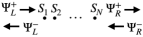
The sample is attached to infinite “leads” and is a scattering region for incoming and outgoing waves in the leads. Each site in the sample is associated with an array of disorder variables. For instance, in the Anderson model with diagonal disorder, would be the onsite potential, i.e., an array of length . The disorder is assumed to be i.i.d. with some normalized probability distribution , and we write disorder averages of any quantity as (any site ) and (the average over all sites).
We assume that each site has a disordered matrix which we parametrize by
| (1a) | ||||
| (1b) | ||||
where and ( and ) are the local transmission (reflection) amplitudes, () are the local transmission (reflection) coefficients, and and ( and ) are the transmission (reflection) phases, which unitarity constrains by and (modulo ). Here and throughout, the subscript indicates dependence on the disorder variables of site . We consider only the single channel case, i.e., the amplitudes are complex numbers and not matrices.
We consider the scattering problem of the -site sample. The matrix for the sample, denoted , relates incoming and outgoing scattering amplitudes in the leads by
| (2) |
The matrix is obtained in the usual way by multiplying the scattering transfer matrices of the sites and converting the resulting scattering transfer matrix back to an matrix (see Appendix A). We write
| (3) |
in which the parameters are constrained by unitarity to satisfy the same equations mentioned below Eq. (1b). No further discussion of the leads is necessary at this point; the problem is to study the sample matrix (3) given the local matrix (1a), which in any particular problem depends on the properties of the sample and leads.
The central object of our study is the joint probability distribution of the minus logarithm of the transmission coefficient (denoted ) and of either one of the reflection phases (we choose the right-to-left phase, ). We focus at first on the localization length and the marginal distributions of and (which indeed are determined by the joint distribution). We write the joint and marginal distributions as
| (4a) | ||||
| (4b) | ||||
| (4c) | ||||
where the subscript on the left-hand side, in departure from our usual convention, indicates dependence on the number rather than on 444Explicitly, we have (e.g.) , where . Due to the disorder being i.i.d., the probability distributions depend only on the number of consecutive sites and not on their location. Also, to make contact with the notation used in the Introduction, we take the spacing between sites to be the unit of distance; then the length of the sample is .. As discussed in the Introduction, for a large sample () the probability distribution of is Gaussian with the mean growing linearly with (although the Gaussian form may not accurately calculate moments of and [42]). The localization length is then determined by
| (5) |
The variance [denoted ] of also grows linearly with , and SPS holds when the mean and variance are related by an equation (see below).
II.2 Review of prior work
In this discussion, we present results from the literature as they apply to our setup, using our notation throughout. We focus on prior work most relevant to our work and do not attempt a comprehensive review. We first review explicit, model-independent results for the localization length and for SPS from the literature, and then we discuss the relation of our work to the literature on the joint distribution.
In Ref. [27], Anderson et al. proposed that there would be a length scale beyond which complete phase randomization would occur. According to this uniform phase hypothesis, for the phase of , which we write as , is distributed uniformly in and independently of . [We will use “uniform” to refer to a phase distribution being uniform over , unless otherwise noted.] This hypothesis yields an explicit formula for the localization length in terms of a local average [27]:
| (6) |
Furthermore, the same hypothesis yields SPS by relating the mean and variance through [27]
| (7) |
However, the uniform phase hypothesis was shown to fail in a number of cases including strong disorder (see [43] and references therein, as well as [44, 45, 46, 47]), multiple scattering channels [48], and anomalies in the Anderson model [49, 50]. In Ref. [34], though, Lambert and Thorpe obtained a more general formula for the localization length that accounts for deviations from phase uniformity:
| (8) |
in which and is any site. Equation (8) recovers the uniform phase result (6) when is uniformly distributed independently of [since ]. In Refs. [34, 35], Lambert and Thorpe furthermore showed that, in a model consisting of randomly spaced delta function scatterers of equal strength, the probability distribution of is generically non-uniform even for an arbitrarily long chain. The second term in (8) makes a substantial correction to the first, particularly for weak disorder. In a more general setting, an expression for the probability distribution of at the zeroth order in disorder strength (with the thermodynamic limit taken before the limit of zero disorder) was derived by Lambert et al. in Ref. [51]; the authors then used this probability distribution in Eq. (8) to find that the localization length is finite in band gaps and infinite outside of band gaps, as expected [51].
The significance of the delta-function model considered by Refs. [34, 35] was challenged by Stone et al. in Ref. [52], in which the authors showed numerically that in the Anderson model with weak, diagonal disorder with vanishing mean onsite energy, the probability distribution of is indeed uniform for large . Stone et al. obtained a formula analogous to (8) for the variance ; using this formula, Eq. (8), and the uniformity of the distribution of , they obtained both the known weak disorder expansion for the inverse localization length and the SPS relation (7). The authors further argued that the delta-function model considered by Lambert and Thorpe is a special case and that any model with the potential being positive as often as negative would yield results similar to those in the Anderson model.
A number of works (including some that we have cited above) have studied the distribution of the reflection phase rather than of . We can understand this as follows. By construction, is distributed uniformly provided that either or both of and are distributed uniformly. The challenging case, then, is what happens when the local phase is non-uniformly distributed: Does the distribution of the sample phase become uniform for large , or not? From here on, we mean by the “uniform phase hypothesis” the assertion that either or both of the sample reflection phases, and , are distributed uniformly for large .
Another approach to the SPS relation was provided by Deych et al. in Refs. [30, 31]. Deych et al. argue that the SPS relation holds in the regime , where is a new length scale that they identify, without appeal to any uniform phase hypothesis. In a setup encompassing both the Anderson model with diagonal disorder and the case of equally spaced delta functions with random strengths [52, 30, 31], Deych et al. provide analytical results in the Lloyd model (i.e., disorder following a Cauchy distribution). They obtain the SPS relation, albeit with an extra prefactor of that they attribute to the peculiarity of the Cauchy distribution; they also present numerical evidence for the SPS relation following from the condition in a more generic model (an array of square well potentials with random widths) [30, 31].
The work with most overlap with ours is that of Schrader et al. in Ref. [32] (see also Ref. [53]), which presents an explicit formula for the inverse localization length and variance and a proof of the SPS relation, all at the leading order in a small parameter. In particular, Schrader et al. proved and , where is given in terms of averages over local quantities [unlike Eq. (8), which includes an average over the whole sample] and where is a small parameter that Schrader et al. identified as “the effective size of the randomness” [32]. The quantity consists of a sum of two terms, one that recovers the uniform phase result (6) at leading order in and a second that contributes due to departures from the uniform phase hypothesis [32]. Schrader et al. point out that although the second term vanishes in the Anderson model (with diagonal disorder and vanishing mean onsite energy), it is in general not a small correction to the first term (for instance, in the random polymer model [54]). Schrader et al. also calculate and to the next non-vanishing order in the Anderson model (), showing that both the uniform phase formula (6) and the SPS relation (7) break down at this order [32].
Let us next review prior work on the joint distribution of and . Given a maximum entropy ansatz, Ref. [55] found that the probability distribution of satisfies a Fokker-Planck equation (which in turn yields a Gaussian distribution for ) 555Reference [55] obtains a Fokker-Planck equation for the probability distribution of . In the localized regime that is our focus, Ref. [55] uses this Fokker-Planck equation to obtain a Gaussian distribution for (there denoted ), as we have stated in the main text. The phase variables in Ref. [55], which are distributed uniformly [c.f. Eq. (2.6) there)], are related to the reflection phases by and [c.f. Eqs. (2.3a) and (2.3b) there].. The maximum entropy ansatz yields a factorization of the joint distribution of and into a product of the two marginal distributions, with the marginal distribution of being uniform. This calculation applies when either or both of the sample reflection phase and local reflection phase are distributed uniformly.
While our work focuses on the case of a single scattering channel (i.e., S matrices), it is useful for further comparison with the literature to consider the case of an arbitrary number of channels ( S matrices). In this more general case, the matrix may be parametrized by transmission coefficients and phases [57, 58]. The generalization of the uniform phase hypothesis to this case is known as the isotropy assumption and is believed to hold when there are many channels () with sufficient coupling between them (see Ref. [59] and references therein). Under this assumption, the joint probability distribution of the transmission coefficients satisfies a version of the Fokker-Planck equation known as the Dorokhov-Mello-Pereyra-Kumar (DMPK) equation [48, 57]. For the case , it has been shown in particular models that the isotropy assumption breaks down and that the transmission coefficients are entangled with the phases in the Fokker-Planck equation [48, 59].
For the case , which is our focus, general and analytical results for the joint distribution of were obtained by Roberts in Ref. [60]; see also Ref. [43]. These works obtained factorization of the joint distribution of into the product of separate distributions for and , apparently in conflict with our result. In Sec. IV, we support our result with analytical calculations and numerical checks, and we provide an explanation for the discrepancy with Refs. [60, 43].
III Scattering expansion of the localization length
III.1 Overview
Our first general result in this paper is a series expansion of the inverse localization length with the local reflection strength as a small parameter. In the course of this calculation, we also present results on SPS and on the marginal distribution of the reflection phase.
Our scattering expansion is defined by rescaling and in the local matrix (1a) (with and also rescaled to maintain unitarity), and, roughly speaking, expanding in the real and positive parameter . (As we discuss below, it is necessary in the calculation to consider the order of limits and in a particular way to maintain the system always in the localized regime. However, this subtlety does not appear in the final results, which may be understood as straightforward expansions in .) For convenience, we let the dependence on be implicit in our notation and refer informally to an expansion in . Thus, the reflection amplitudes and are both first order and the reflection coefficient is second order. While we assume for now that is linear in the small parameter , we explain below the simple modifications to our results in the more general case of starting at linear order but also having higher-order corrections.
Before presenting our calculation, we first note that the result of Schrader et al. [32] mentioned in the previous section has the following corollary: our parameter is a valid choice for their parameter , and their formula for the localization length and variance may be written in terms of local averages at any site as (see Appendix B for the calculation) 666In the case of and , a result related to Eq. (9) has also been obtained in Refs. [93, 94, 95] using the WSA approach developed there. See Appendix C for details.
| (9) |
and
| (10) |
where we have also improved their results from error to error (see next paragraph). The first term on the right-hand side of Eq. (9) is the small expansion of the uniform phase result (6), while the second term is the contribution from deviations from the uniform phase hypothesis. We emphasize again that the second term is not, in general, a small correction to the first; indeed, both terms are of the same order in the small parameter. We also note that unlike the Lambert and Thorpe formula (8), Eq. (9) involves only local averages and no averaging over the whole chain.
In writing Eqs. (9) and (10), we have in fact gone beyond the immediate corollary of the result of Schrader et al., which would yield the leading order contributions as given above but with error instead of 777In the particular case of the Anderson model with onsite disorder with vanishing mean, Ref. [32] calculates the third and fourth order terms and finds that the third order terms indeed vanish.. The third order terms, and indeed all odd orders, vanish due to the following symmetry argument. The localization length and variance must be invariant under phase redefinitions of the incoming and outgoing scattering amplitudes; in particular, we can redefine (), which sends and . It follows that and must appear in equal numbers in each term (hence there are no terms of the order of an odd power of ). This argument relies on the existence of series expressions for and with coefficients involving only local averages of integer powers of , , , and (note that the latter two are invariant under the phase re-definition). In this section we show that such a series exists for , and in Sec. IV we show it for .
We have thus explicitly connected SPS to the weakness of the local reflection strength, and we have extended the SPS relation to one more order [Eq. (10)]. Our next task is to apply the scattering expansion to the inverse localization length, recovering Eq. (9) and providing a recursive calculation of higher orders. We show that all orders of the series depend, as in Eq. (9), only on averages involving the local reflection amplitudes and . We explicitly verify the vanishing of the third order and present the next non-vanishing order ().
A key ingredient in our calculation is the limiting form as of the probability distribution of the reflection phase, which we write as
| (11) |
(In Appendix D, we show that this limit exists given the assumption that localization occurs.) Our approach is based on the following series formula, which we derive below, that expresses the inverse localization length in terms of the Fourier coefficients and the moments of :
| (12) |
Equation (12) is related to the Lambert and Thorpe formula (8), with the essential difference being that we focus on the distribution of rather than and work in frequency space. Note that the uniform phase formula (6) is recovered from Eq. (12) in two non-exclusive special cases: (i) the local reflection phase is uniformly distributed independently of the local reflection coefficient (then for ), or (ii) the reflection phase distribution of the sample is uniform. Case (i) is an example of strong phase disorder. The difficulty of applying Eq. (12), in the case that (i) does not hold, is that it has been shown in many examples that the reflection phase distribution can be non-uniform (see references cited in Sec. II.2) and in general the distribution is only known numerically (although Schrader et al. [32] calculated in an equivalent form).
In order to use Eq. (12), we calculate the probability distribution of the reflection phase order by order in the scattering expansion. We show that the zeroth-order contribution is (generically) the uniform distribution, and that at any fixed order of the expansion, only finitely many of the Fourier coefficients are non-vanishing. We further show that the expansion coefficients are local averages that can be calculated recursively. Together with Eq. (12), this recursive expansion of the Fourier coefficients yields our scattering expansion of the inverse localization length.
In the remainder of this section, we derive the above results (Sec. III.2), then apply them to disordered wires (Sec. III.3) and to quantum walks (Sec. III.4). We note here that our calculation in this section only concerns the localization length and not the variance; however, we do obtain Eq. (10) by a different approach in Sec. IV, and it is convenient to apply this result in this section to comment on SPS in a broad class of PARS.
III.2 General calculation
We compare a sample of size with a sample of size using the following exact relations between the transmission coefficients and reflection phases (for completeness we derive them in Appendix A):
| (13a) | ||||
| (13b) | ||||
A basic assumption of our calculation is that localization occurs: that is, for large the sample reflection coefficient in all disorder realizations 888Whenever we require a property to hold for all disorder realizations, we expect that it would also suffice for that property to hold for almost all realizations (i.e., all except a set of measure zero).. We can then replace in the logarithm of Eq. (13a) and in Eq. (13b); in other words, we keep and constant terms, but neglect terms linear or higher in . We thus obtain
| (14a) | ||||
| (14b) | ||||
where
| (15a) | ||||
| (15b) | ||||
Let us pause to present an intuitive picture, in which we temporarily think of the increasing sample size as representing time. Then, Eq. (14b) indicates that the reflection phase performs a random walk on the circle; furthermore, the probability distribution of the step size depends on the current position that the walk has reached. From this point of view, it is clear that the long-time distribution of the phase should generally be non-uniform, since the walk will spend more time in regions where the step size is smaller. From Eq. (14a), we see that the variable performs a random walk on the half-line with a step size that depends on the current position of the phase walk, though not on the current position of . While the average position reached by after a long time may be obtained by treating the phase as simply another disorder variable in the step size (i.e., sampling the phase from its long-time distribution), the variance of and the correlations between and the phase seem to require a more careful treatment (Sec. IV).
To clarify a technical point about our expansion, we temporarily restore the true small parameter . While we are interested in the regime of small , we cannot simply expand in for fixed , since the point corresponds to a sample transmission coefficient of unity, inconsistent with our replacing . Instead, we must suppose that for any fixed , there is some sufficiently large for which the sample transmission coefficient is negligible for any in every disorder realization [63]. [ is of order of the localization length, so in view of our results below, it will turn out that .] All expansions in powers of in our calculations below must be understood as occurring in the regime of with 999A similar point is mentioned in Ref. [26] (footnote 24).. This subtlety need not be considered in our final answer for , and we have there a simple expansion in .
We make a few comments now about our conventions. Here and throughout we use a superscript to indicate the order in (i.e., for any quantity ). Also, since the disorder is i.i.d., we frequently replace the disorder average over site by an average over any site . Finally, all phases are constrained to be in , and any equations between non-exponentiated phases are to be understood as holding modulo .
Next, we develop the scattering expansion for the Fourier coefficients . A recursion relation for is determined by , from which Eq. (14b) then yields
| (16) |
We then send and take the Fourier transform of both sides to obtain [noting Eq. (15b)]
| (17) |
where we have defined
| (18a) | ||||
| (18b) | ||||
Eq. (17) can be solved order by order in the scattering expansion, as we now show.
We write the expansions of and as and , with corresponding expansions for the Fourier coefficients. Note that by the normalization condition, , we have for all .
We now equate terms of the same order on both sides of Eq. (17). Since , the quantity appears on both sides of the order equation (for any ). This has two immediate consequences. First, the zeroth-order part of Eq. (17) is
| (19) |
and second, for any , the order part of Eq. (17) for can be re-arranged to
| (20) |
where [and where we have written as a sum over Fourier coefficients].
Equation (19) implies (see next paragraph) that for all . The Fourier coefficient is fixed by the normalization of the probability distribution, so we find that the zeroth-order distribution is uniform:
| (21) |
Equations (20) and (21) rely on assumptions of “reasonable” disorder and “generic” model parameters, as we now explain. For instance, the limit of no disorder at all technically meets our definitions so far, but must be excluded. Also, in applying our approach to any particular model, we must consider the model as part of some family of models (e.g., with parameters taking a continuous range of values), since our results are expected to hold generically but may break down at some special values of parameters (the anomalous momenta of the Anderson model are an example). A precise statement of these assumptions is (a) that localization occurs (an assumption that we have used already), and (b) that the following inequality holds for all integers :
| (22) |
where is any site. We expect that any choice of disorder distribution and model parameters that violates (22) is “non-generic” (since a particular alignment of reflection phases across disorder realizations is required). [In Appendix F, we consider the case that (22) is only assumed for for some finite .] Noting that , we see then that for , we have , so indeed Eq. (19) implies and the denominator in Eq. (20) is non-vanishing.
Equation (20) is almost in a form in which we can calculate the reflection phase distribution to many orders. The point is that the right-hand side involves only the reflection phase distribution at lower orders than the order on the left-hand side; thus, in principle we can start with Eq. (21) and iterate Eq. (20) to calculate higher orders. To make this process more efficient, we show next that only finitely many Fourier coefficients are non-vanishing at any given order. In particular, we show that for any ,
| (23) |
and we show that the sum over on the right-hand side of Eq. (20) can be truncated to a finite sum:
| (24) |
The Fourier coefficients that we need are easily calculated to many orders from the definition (18b), and the positive frequency coefficients () can be obtained from .
To derive Eqs. (23) and (24), we use some simple properties of the function . We start by noting that for . Suppose now that for some , when and [this holds for by Eq. (21)]. Then the only terms on the right-hand side of Eq. (20) that can be non-zero are those with and , which implies for these terms. Thus, Eq. (23) holds by induction. The sum over in Eq. (20) can therefore be truncated to to . Fixing , we can see that the negative terms can be dropped since for ; thus we obtain Eq. (24). Further improvement (dropping terms in the sum that must be zero) is possible, but Eq. (24) suffices for our purposes.
We can now calculate higher orders of the reflection phase distribution in a completely mechanical, recursive fashion using Eq. (24), starting from . To present compactly the first few terms of these expansions, we use the following notation:
| (25a) | ||||
| (25b) | ||||
| (25c) | ||||
| (25d) | ||||
| (25e) | ||||
Then we obtain, transforming back from frequency space (see Appendix F for further detail)
| (26) |
which shows explicitly the corrections to the uniform distribution that is obtained at zeroth order. Let us also note that interchanging in Eqs. (25b)–(25e) yields the corresponding expression for the limiting distribution of the left-to-right reflection phase ().
We proceed to use the reflection phase distribution to calculate the inverse localization length in the scattering expansion. We start by deriving the relation (12) between the localization length and the Fourier coefficients . From the recursion relation (14a) for , it follows that for sufficiently large , increases by the same constant amount (which by definition is ) each time is increased by one:
| (27) |
The site on the right-hand side can be replaced by any site , since the disorder is by assumption distributed identically across the sites. We thus obtain an expression for the inverse localization length in terms of the reflection phase distribution:
| (28a) | ||||
| (28b) | ||||
Equation (28b) can also be obtained directly from the Lambert and Thorpe expression [Eq. (8)], or (using the correspondence discussed in Appendix B) from the Furstenberg formula quoted in Ref. [32]. Expressing the second term in frequency space is straightforward [65] (see Appendix E) and yields Eq. (12).
Since the odd orders vanish due to the symmetry argument presented below Eq. (10), we may write
| (29) |
where the superscript indicates the order in the expansion. Furthermore, for any , Eq. (12) yields
| (30) |
where we noted that Eq. (23) allows us to drop the terms to in the sum. Reading off the Fourier coefficients from Eq. (26), we then calculate the first two non-vanishing orders of the scattering expansion for the inverse localization length (the main result of this section):
| (31) |
On the right-hand side, the first two terms are second order and recover Eq. (9). The remaining terms are fourth order. We have explicitly checked [using Eq. (12)] that the third- and fifth-order contributions vanish, consistent with the general symmetry argument. Our recursive formula (24) can straightforwardly generate still higher orders of Fourier coefficients , and thus of .
A final technical point is that we have so far assumed that is strictly linear in the small parameter . However, it may be the case in a particular problem that starts at linear order in some parameter but also has higher-order corrections in (for instance, this occurs in the Anderson model, where is essentially the disorder strength). There are two straightforward steps to adapt the results of this section to this more general case. First, the condition (22) is required to hold at the zeroth order in as . Second, the series for is to be truncated to a fixed order in , which implies in particular that each term at a given order in the expansion contributes generally at all orders in .
III.3 Application to disordered wires
In this section, we apply our general results to the Anderson model and to a broad class of PARS. In the Anderson model, we consider the case of diagonal disorder (i.e., disorder in the onsite energies but not the tunneling) and show that our next-to-leading order result (31) agrees with and extends a known formula for the weak disorder expansion of the inverse localization length. We also verify our result for the probability distribution of the reflection phase with the literature, and we discuss the “anomalous” values of the momentum. In the PARS case, we use the Born series to show that Eqs. (9) and (10) demonstrate the SPS relation to the first two orders in the potential strength. As a special case, we obtain the SPS relation in the same square well array model considered by Deych et al. (see Sec. II). We also verify our higher-order formula (31) for the inverse localization length by comparing to another special case in the literature.
III.3.1 Anderson model with diagonal disorder
As a first application and check of our general results, we consider the Anderson model: a one-dimensional tight-binding chain with disordered onsite energies. The well-known scattering setup for this problem is the following:
| (32) |
where the onsite potentials are i.i.d. for inside the “sample” region (defined as the sites ) and zero otherwise ( and ). We take . The Schrödinger equation for an eigenstate with energy can be written in transfer matrix form:
| (33) |
where
| (34) |
The clean Hamiltonian has spectrum , and given a fixed we can write a scattering state with energy as
| (35) |
The phase convention for the amplitudes on the right (i.e., the factors of [66]) is chosen so that the local reflection phase takes the same form at every site (i.e., it depends on but not on the integer value of the site index ), which in turn results in the existence of a limiting distribution of the reflection phase as . Were we to omit the factors of , the distribution would instead tend to a fixed function evaluated with an -dependent shift of its argument and hence would not strictly have any limit.
To convert position-space amplitudes to scattering amplitudes, define a matrix as
| (36) |
Then,
| (37) |
Chaining transfer matrices then yields the desired product form of the scattering transfer matrix of the sample:
| (38) |
where
| (39a) | ||||
| (39b) | ||||
where we have defined a dimensionless onsite energy:
| (40) |
The corresponding matrix at site is
| (41) |
from which we read off the reflection amplitudes
| (42) |
Thus, our scattering expansion applies in the regime of weak onsite energies. We assume that almost all disorder realizations have , where is a fixed constant independent of the realization. Note in particular that we are not considering any long-range probability distribution (such as the Cauchy distribution considered by Deych et al. in Refs. [30, 31]). The parameter that controls the reflection strength can be taken to be , and we refer informally to an expansion in .
Our main result for the Anderson model is obtained by substituting the reflection amplitudes (42) into Eq. (31). With no loss of generality (see below), we take the mean onsite energy to be zero (), yielding
| (43) |
The terms in the first line of (43) recover the known expansion to fourth order 101010See, e.g., the second unnumbered equation below Eq. (36) in Ref. [32] (which cites earlier work). Our Appendix B provides some details for converting the notation of Ref. [32] into our notation.. The fifth-order term in the second line is the leading dependence on the asymmetry of the probability distribution of the onsite energy, in particular its skewness (i.e., third moment). We are able to calculate the fifth order term here because there is no term of fifth order in the reflection strength in Eq. (31).
We note that Eq. (43) is consistent with the work of Ref. [68], which considers an asymmetric distribution with (in our notation) , , and a small . Reference [68] finds that the non-vanishing skewness has no effect at leading order on the inverse localization length.
The result (43) might be expected to hold more generally, in particular with periodic or open boundary conditions instead of the scattering setup that we used. As a consistency check of this expectation, we consider the localization length as a function of the eigenstate energy and the average onsite energy: , where . With periodic or open boundary conditions, the average onsite energy is just an additive constant in the Hamiltonian, so we must have the symmetry property . We have verified that our scattering calculation also has this symmetry property [by evaluating Eq. (31) with general and comparing to Eq. (43)] up to error . Note that here.
We emphasize that the equivalence of across different boundary conditions must break down if we allow to be sufficiently large in sufficiently many disorder realizations (e.g., by taking to be large or by having large variations about ), for then the scattering setup has an attenuation effect (see next paragraph) that is not present in the problems with periodic or open boundary conditions. This regime is outside the scope of our calculation, since the reflection strength approaches unity. We do not know if the difference between boundary conditions can be detected at sufficiently high order in the scattering expansion, but due to the symmetry property mentioned in the previous paragraph, we expect that Eq. (43) holds also for periodic or open boundary conditions.
To explain this point in more detail, we consider first the clean limit with strong onsite energy (all ). In the case of periodic or open boundary conditions, is of no significance and the localization length is infinite. However, with scattering boundary conditions, the transmission coefficient decays exponentially in purely because of attenuation. More generally, in the course of a strong disorder calculation, Ref. [69] shows that the transmission coefficient (with any disorder such that all are large) is simply proportional to the product of over all sites , from which it follows that in the scattering setup; however, this cannot be the answer in the periodic or open setups because setting all to be equal yields a non-zero .
Next, we calculate the probability distribution of the reflection phase up to errors of third order in , verifying our answer with the literature in the special case of . Here we do not see any obvious symmetry relation between the problem with and the problem with small, non-zero .
For convenience, we define
| (44) |
We then obtain
| (45a) | ||||
| (45b) | ||||
which we substitute into Eq. (26) to obtain the probability distribution of the reflection phase up to second order (the third-order term may be obtained similarly). In particular, the leading correction to phase uniformity is
| (46) |
For , the first-order term vanishes, and the leading correction is second order:
| (47) |
in agreement with Ref. [70], where a symmetric exponential distribution for is considered. Equation (47) also agrees with Ref. [60], which considers an arbitrary disorder distribution symmetric about zero, except for the sign of the term (and our sign agrees with Refs. [70] and with numerical checks) 111111Here we explain the comparison with Refs. [70] and [60] in more detail. From Eq. (4.21) of Ref. [70], we see that the coefficients there are related to our notation by . We specialize to the symmetric exponential distribution with width by setting , yielding agreement with Eq. (4.23) there. To compare with Ref. [60], we note from Eq. (54) there that in our notation, and we integrate over in Eq. (55) there to obtain , i.e., the distribution of . By Eq. (42), we have , resulting in the sign discrepancy mentioned in the main text.. Since Eq. (46) contains a term linear in , it cannot be recovered from Eq. (47) by a simple shift of energy.
We conclude this section by discussing the special case of anomalous momenta. So far, we have assumed that the momentum takes a “generic” value within (recall that the lattice spacing is the unit of distance). In particular, the condition (22) at the zeroth order in [see the discussion below (22)] is
| (48) |
which excludes for some integers . These special points are known in the literature as anomalous (see Ref. [50] and references therein).
Let us consider with reduced to simplest form and with . Then (48) holds for , but not for . The calculation in Appendix F then shows that Eq. (43) holds provided that . More generally, our approach can be used to calculate the inverse localization length up to and including order in . (The increase, with , in the expansion order affected by the anomaly has already been discussed in Refs. [72, 73, 74].) As a check, we note that at the band center anomaly [75] ( and hence ), the scattering expansion does not yield even the leading order (); this is consistent with the known result that the leading order formula is modified at the band center [75]. Furthermore, Ref. [50] finds that the leading order formula holds at all of the anomalies except the band center and band edge, which is consistent with what we find above (since except at the band center and edge).
III.3.2 Periodic-on-average random potential
Setup.
We consider the problem of a free particle scattering off identically and independently disordered potentials with disorder also in the separations between the potentials. Since the separations are not necessarily constant (though we may choose them to be as a special case), the scattering region is in general periodic-on-average rather than periodic.
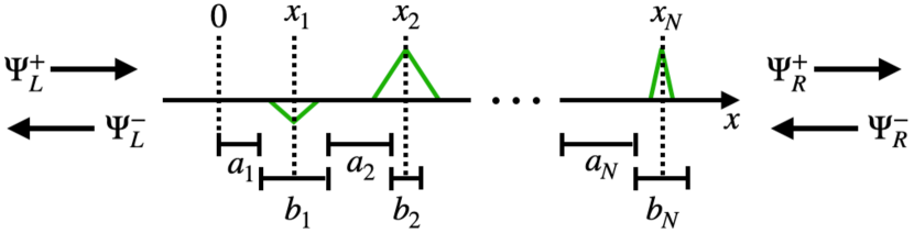
To define the problem, we consider a family of potentials , where is an array of parameters characterizing the potential, and where all potentials in the family have a fixed range independent of [that is, for ] 121212We can expect our results to hold also if the potentials are sufficiently small (e.g., exponentially decaying) for .. We form a chain of such potentials, with “promoted” to a site-dependent array and with the th potential centered at some position :
| (49) |
where . We set the centers to be at , where and may be disordered arbitrarily as long as the potentials never overlap (). Thus, we have a sequence of regions of varying widths which are separated by spacings (see Fig. 2).
We collect the parameters of site into a single array and assume that are i.i.d. (allowing correlations between the individual elements of ).
In any particular disorder realization, we consider a scattering eigenstate with energy , writing the wavefunction outside the sample as
| (50) |
where . With this choice of phase convention, we may bring the scattering problem into the required form for applying our general results. Indeed, we show in Appendix G.1 that if the single-site scattering problem of the potential [i.e., Eqs. (49) and (50) with , , and ] has reflection amplitudes and , then the scattering transfer matrix of the chain may be written as
| (51) |
where the local scattering transfer matrix is equivalent to an matrix which has reflection amplitudes and given by
| (52a) | ||||
| (52b) | ||||
Thus, given the reflection amplitudes of the single-site problem, we can apply our general results to the general PARS problem defined above. We note here that throughout this section, the localization length is expressed in units of the average lattice spacing (and thus should be multiplied by to restore physical dimensions).
From Eqs. (52a) and (52b), we see that and may be understood as phase disorder, at least in the case when they are distributed independently of the parameters characterizing the potential. If or is strongly disordered, the uniform phase result (6) is obtained; for we can see this from Eq. (12), while for we can use Eq. (12) with the roles of and interchanged.
A comparison with the literature.
We verify our fourth-order result for the inverse localization length with the literature in the following special case. Consider the case of identical potentials with disorder only in the separations between the centers of the potentials; that is, set all and , so that all , all , and all (where we recall that the hat indicates the variable for the single-site scattering problem). For notational convenience, define (for )
| (53) |
Then Eq. (31) yields
| (54) |
in agreement with a result by Lambert and Thorpe [35] (see Appendix G.2 for details).
SPS relation.
Returning to the general case, we use the usual Born series to obtain the single-site scattering amplitudes in terms of the Fourier transform of the potential []:
| (55a) | ||||
| (55b) | ||||
Here and in the following we are really expanding in some site-independent potential strength that all are proportional to. The dimensionless small parameter is of order , but for short we continue to refer to an expansion in .
Note that the reflection strength starts at linear order in but also has quadratic and higher corrections from higher terms in the Born series. Equations (9) and (10) then show that the inverse localization length and variance each start at second order () and have third-order () corrections that must be equal, due to the absence of terms in (9) and (10). Thus, even without calculating the term explicitly, we have obtained
| (56) |
Equation (56) thus demonstrates the SPS relation (7) for a broad class of periodic-on-average random systems up to the first two (generally non-vanishing) orders of the potential strength, and . Let us note that Eq. (56) at the leading order [i.e., with the error term as ] follows straightforwardly from the result of Schrader et al. [32]; our work rules out terms in Eqs. (9) and (10), which in turn rules out any term in Eq. (56).
As a special case, we may apply Eq. (56) to a model used by Deych et al. in Refs. [30, 31] to provide numerical support for their approach to the SPS relation. The model, which is defined in more detail in Ref. [39], has classical light passing through alternating regions with dielectric constants and ; the regions have fixed widths and the regions have i.i.d. disordered widths. This problem maps exactly to a quantum problem with square-well potentials, as we now explain. While Refs. [30, 31, 39] used a position-space transfer matrix setup, we instead use a scattering setup in which the “leads” to the left and right of the sample are regions. We recall that the indices of refraction in the two regions are (), and we set without loss of generality. Then this classical problem is equivalent to a quantum scattering problem of the form (49) with all , 131313This model provides an example of correlations between the parameters of , which are allowed in our setup. In particular, the parameters of the square well potential are first promoted to site-dependent parameters . We then set all and ; in , the potential width is thus correlated with the width ., and (the mass is arbitrary). Thus, Eq. (56) yields the SPS relation in the regime of the two dielectric constants and being close to each other, with arbitrary disorder strength in the widths .
Inverse localization length at leading order.
At the leading order in the potential strength, Eq. (9) yields
| (57) |
In the case of equal spacings between the centers of the potentials, Eq. (57) simplifies to yield the variance of . [A similar result is known for continuous random potentials; see, e.g., Eq. (2.84) of Ref. [78].] Indeed, setting all and yields
| (58) |
The first term is the only one present when the uniform phase hypothesis holds. Thus, we disagree with the expectation in Ref. [52] that the uniform phase hypothesis [and thus Eq. (6)] should hold for any potential that is positive as often as it is negative 141414For a definite counterexample, consider , i.e., an array of delta function potentials with random strengths. If , then Eq. (6) is not correct at leading order in weak disorder, even if ..
The next three orders in in the inverse localization length may be obtained from Eq. (31) and from the next order in the Born series for the single-site reflection amplitudes, but we have not done this calculation.
Transparent mirror effect.
As a particular application of our results, we consider an array of square-well potentials with equal strengths and with spacings and widths that are disordered independently (Fig. 2b). This model is equivalent to a classical optics problem in which light scatters on a disordered Bragg grating (i.e., a chain of dielectric slabs); the strong reflection that occurs due to localization, even if the individual dielectrics have weak reflection coefficients, is known in that context as the transparent mirror effect [80]. This Kronig-Penney–type model has been studied by a number of approaches (e.g., Refs. [81, 39, 82, 83, 84]), and the model used by Deych et al. is a particular case. The transparent mirror effect has recently been studied in twist-angle-disordered bilayer graphene in Ref. [85], although it seems that our results do not apply to the model considered there because the disorder couples neighboring S matrices.
We thus consider the scattering problem for the quantum Hamiltonian (49) with . Let us recall the correspondence to the classical optics problem. A free quantum particle with momentum has its momentum change to in a region of constant potential , while for light passing through a region with constant index of refraction (we use a tilde to avoid confusion with the site index ) we instead have the free momentum changing to . We thus read off the correspondence . We cover both cases by defining
| (59a) | ||||
| (59b) | ||||
and we assume throughout (which corresponds to real momentum ).
Our results apply to the more general case in which (in addition to and ) is also disordered; the only requirement is that the disorder parameters are i.i.d. For simplicity, we are focusing on the case of and independent disorder in and .
To use our general results, we first recall the reflection amplitudes for scattering on a rectangular potential of strength (or, equivalently, an index of refraction ) from to . The reflection amplitudes and reflection coefficient are
| (60a) | ||||
| (60b) | ||||
and
| (61) |
When we expand these terms in small using Eq. (59b), we do not expand the term that appears in and for two reasons: (a) this makes a symmetry property (that we discuss below) more manifest, and (b) this expansion can fail to commute with the strong disorder limit in some cases (e.g., a flat disorder distribution for ).
Equations (9), (52a), and (52b) then yield our main result for the transparent mirror problem:
| (62) |
The distinctive feature of this result compared to prior work is that the spacings and widths can be disordered arbitrarily. While the term has the same dependence on disorder as the term, the and terms [which may be obtained from the higher-order result (31)] have different dependence on disorder; we omit these lengthy expressions.
Equation (62) satisfies a consistency check based on symmetry, as we now summarize (see Appendix G.3.1 for details). By considering an alternate scattering problem in which the leads are regions and the scatterers are regions, we show that each order in of must be symmetric under the exchange
| (63) |
which indeed is true for Eq. (62). We have verified that the and corrections also satisfy this symmetry. Another consistency check is that we obtain in the case of no disorder.
We have also compared with some analytical results from the literature, as we now summarize (see Appendix G.3.2 for details). Reference [80] obtains the uniform phase result (6) in the case of strong disorder in [c.f. Eq. (52a) and the discussion below there for how we obtain the same result]. Reference [82] treats exactly, with weak disorder in and no disorder , and we find that their result agrees with Eq. (62) in the regime of overlap. Finally, in Ref. [81], and are considered to follow exponential distributions, with arbitrary disorder strength, and is treated at the leading order. The result is of the same form as what we obtain from Eq. (62), but seems to have different numerical factors.
Using Eq. (62), we can show analytically that the inverse localization length can have non-monotonic dependence on disorder strength for some choices of disorder, e.g., both and uniformly distributed in an interval with varying disorder strength . The special case of all can alternatively be treated using Eq. (54) (note that one must replace there to account for the finite width of the scatterers). Then, a uniform distribution in (for example) exhibits non-monotonicity, as is also clear from the numerical results of Ref. [83].
III.4 Application to discrete-time quantum walks
We consider a general two-component, single-step quantum walk in one dimension. We explore the effect of phase disorder on the localization length using Eq. (31), showing in particular that the dependence on disorder strength can be non-monotonic. We verify our results with the literature in the limits of weak and strong phase disorder and also with numerics.
The setup is an infinite chain with site index and an internal “spin” degree of freedom ( or ). The “shift” operator moves the two spins one step in opposite directions:
| (64) |
The unitary operator that implements a single time step is , where the “coin” operator acts as a unitary matrix on the spin degrees of freedom at each site. We focus on the case of a coin operator that acts on each site independently:
| (65) |
where is a unitary matrix. Following Vakulchyk et al. [18], we parametrize the general coin matrix as
| (66) |
where the site-dependent (and possibly disordered) phases , , may be interpreted as potential energy, external and internal synthetic fluxes, and kinetic energy, respectively [18].
The stationary state equation may be brought to a transfer matrix form even though a transfer matrix would be expected (for a bipartite lattice with nearest-neighbor coupling) [18]. Indeed, writing a general state as and defining a two-component wavefunction (note that the component is offset by unit), one finds that the stationary state equation is equivalent to
| (67) |
where
| (68) |
is the transfer matrix [18].
To bring the problem into a scattering framework, we define a disordered “sample” occupying sites of the chain by taking to have i.i.d. disorder, possibly including correlations between the phases , , , and at a given site . We will see below that in order to be in the weak reflection regime captured by our general calculation, we must take to be small, which corresponds to a highly biased coin. The remaining phases , , and are arbitrary, and in particular we can explore the crossover between weak and strong disorder in these phases.
Given the disordered sample as we have defined it above, there are many possible scattering problems corresponding to different choices for a site-independent array to be assigned to in the “leads” (i.e., for and for ). We find it convenient to set , and we refer to this setup as “Tarasinski leads,” since the same is done by Tarasinski et al. in Ref. [33]. We show in Appendix H that for samples long enough to be in the localized regime, other choices of leads result in the same probability distribution of (in particular the localization length is independent of the choice of leads).
We proceed to set up the scattering problem with Tarasinski leads, which have a linear quasienergy spectrum. A scattering solution to the stationary state equation may be written outside the sample as (see Appendix H for details)
| (69) |
where . With this choice of phase convention, we have
| (70) |
and so,
| (71) |
We thus obtain the scattering transfer matrix of the sample as with . It may be verified that satisfies the psuedo-unitarity condition (which confirms that is a valid scattering transfer matrix). The corresponding matrix is , i.e.,
| (72) |
We can thus apply our results to the problem of scatterers with the single-site matrix given by (72). [Indeed, since any unitary matrix can be parametrized as in Eq. (72), the DTQW we are considering in fact represents the most general problem that our results apply to.]
From Eq. (72), we read off the single-site reflection amplitudes and reflection coefficient. The expansion parameter in our formalism is thus . The generic condition (22) reads
| (73) |
which indeed holds for all non-zero integers except in the special case that is non-disordered and is a rational multiple of . Although we ignore this special case from now on, our explicit results below are still valid there unless the rational multiple is of a particular form (see Appendix F).
Up to second order, Eqs. (9) and (10) yield the inverse localization length and variance:
| (74a) | |||
| (74b) | |||
To present the inverse localization length to fourth order in a compact form, we use the notation
| (75) |
and we note that . Then Eq. (31) yields our main result for the DTQW:
| (76) |
in which the first two terms recapitulate Eq. (74a). Note that the external synthetic flux does not appear (as noted by Ref. [18]).
Next, we specialize Eq. (76) to various choices of disorder, checking our results with the literature and pointing out cases in which the localization length depends non-monotonically on disorder strength. For each choice of disorder, we only need to calculate the coefficients defined in Eq. (75). Throughout, we present only the localization length, bearing in mind that the variance may be obtained at the leading order from Eq. (74b).
III.4.1 Disorder in individual phases.
Here, we follow Ref. [18], introducing disorder in one phase variable at a time.
Consider first the case of disorder in only, with and . We obtain
| (77a) | ||||
| (77b) | ||||
where the second line specializes to a flat disorder distribution of width (i.e., uniform in ), and where .
We now check our result (76) with the literature in the limits of weak and strong disorder. For weak disorder with , we obtain , which agrees with the small expansion of a result from Ref. [18] [see their Eq. (26), recall the dispersion relation , and note that for the flat disorder distribution] except for an overall constant factor of 151515In the special case of weak disorder in , Ref. [18] mentions a factor of discrepancy between their analytical and numerical results for [see below their Eq. (29)], and it is in the right direction to agree with our result. We believe that this factor of is also present in their analytical calculations for weak disorder in or in , as removing it restores agreement with our results in those cases as well. The factor of that appears in our convention of presenting the localization length in the form has been accounted for in this discussion and is not the source of the discrepancy.. In the strong disorder limit (i.e., the flat distribution with ), we get , in agreement with the small expansion of another result from Ref. [18], namely [their Eq. (48)]
| (78) |
Equation (78) (for any ) may also be obtained from our Eqs. (12) and (72); in our setup, this is a case in which the uniform phase result (6) holds because the local reflection phase is uniformly distributed independently of the local reflection coefficient. In passing, we note that if there is disorder in as well (independent of the strong disorder in ), then Eq. (78) generalizes to (and indeed the same result is obtained if the strong disorder is in instead of ).
At the band center () anomaly noted by Ref. [18], we obtain , whereas the expansion of the result of Ref. [18] for small yields the same answer with prefactor [or if the factor of [86] is corrected]. Unlike the Anderson model anomalies mentioned above, in this case we expect our result to apply, since our assumptions are met [i.e., localization occurs and the inequality (73) holds].
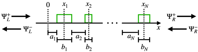
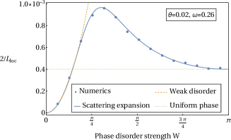
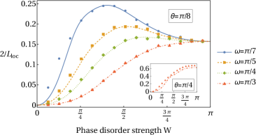
Equation (76) thus interpolates, in the regime of strong coin bias, between the known limits of weak and strong disorder (see Fig. 3a). In certain ranges of quasienergy , the dependence on the disorder strength is non-monotonic. Although strictly speaking we have assumed to be a small parameter, we find favorable agreement with numerics even for only a moderate amount of coin bias (e.g., ); see Fig. 3b.
For definiteness, we present the inverse localization length at second order [Eq. (74a)] with the flat distribution:
| (79) |
which seems to qualitatively capture the non-monotonicity in [although including the terms in Eq. (76) improves the agreement with numerics].
In the case of disorder in only, with and , we obtain
| (80a) | ||||
| (80b) | ||||
where the second line specializes to uniform in . In this case, the inverse localization length (76) depends on disorder monotonically, with a simple leading order expression . We again agree with Ref. [18] in the limits of weak and strong disorder once their results are expanded in . Indeed, for weak disorder with , we find , in agreement with their Eq. (29) [86]. For strong disorder, Ref. [18] again obtains Eq. (78), which we recover in the same sense as mentioned above.
Finally, we consider disorder in the coin parameter , with . In this case we can only access the weak disorder regime, since our expansion is in small . We write , where is, e.g., uniformly distributed in . We obtain and , in agreement with Ref. [18] [see their Eq. (31) [86]].
III.4.2 Alternate form of phase disorder
We now specialize to a case studied experimentally in Ref. [9] and theoretically in Ref. [19]. Again we verify our results with the literature in the limits of weak and strong phase disorder, and then we explore the full range of disorder and find that the localization length in certain ranges of quasienergy is non-monotonic as a function of disorder strength.
The coin matrix in Ref. [19] is, in our notation,
| (81) |
where , are constant phases and , are disordered phases. The coin matrix of Ref. [9] is obtained by shifting and .
We specialize to the case (81) by setting , , , and . Then the inverse localization length up to error of sixth order in is given by Eqs. (75) and (76) with the above substitutions.
Our result agrees with Ref. [19] in the regimes of overlap, as we now explain. In the case of weak disorder with vanishing mean and no up-down correlation ( and ), we obtain , in agreement with the small expansion of a result 161616See Eq. (11) of Ref. [19], where is our and is our . from Ref. [19]. In the case of strong disorder, i.e., and independently and uniformly distributed in , we obtain , in agreement with the small expansion of another result from Ref. [19], namely Eq. (78) [Eq. (10) there]. Eq. (78) may also be obtained directly just as in the cases mentioned above of strong disorder in or (and has the same generalization to the case of independent disorder in ).
We thus interpolate, in the regime of small coin parameter, between the known limits of weak and strong phase disorder. For definiteness, we present now the leading order result, first for general phase disorder and then for the case of being independently and uniformly distributed in . Equation (74a) yields
| (82a) | ||||
| (82b) | ||||
Note that in the regime of or , there is a value of phase disorder strength beyond which any further increase in disorder strength (up to the maximum ) increases the localization length.
IV Joint probability distribution
We proceed to apply the same scattering expansion approach to the joint probability distribution . We present and discuss the results first, then the analytical calculation and numerical checks.
IV.1 Overview of results
Our main result is the following general form for sufficiently large sample length : there is a constant and two functions , for which we have
| (83) |
where the phase-dependent variance grows linearly with and has a sub-leading, phase-dependent correction:
| (84) |
For large , the marginal distribution determined by Eq. (83) takes the known Gaussian form:
| (85) |
where the slope of the variance is determined by the same constant :
| (86) |
Equation (83) may be understood as the statement that the conditional distribution of given is Gaussian for large . Furthermore, the leading behavior of the mean and variance is linear in with slope independent of the phase.
We obtain Eq. (83) to all orders in the scattering expansion by a calculation described in the following section. This calculation, which relies on some assumptions (that we discuss below), provides a procedure for calculating all parameters and functions that appear in Eq. (83) order by order in the scattering expansion (with coefficients only involving local averages), except that the functions and each have a -independent additive constant that is not determined. [These constants appear in the error terms in Eqs. (85) and (86).] The expansions for and have already been presented in Sec. III; here we develop similar recursive expansions for , , and .
A notable feature that we demonstrate for the function is that it coincides, at leading order and up to a factor of , with the first order correction to uniformity in the phase distribution . In particular, we recall from (26) that the phase distribution is given at first order by , where
| (87) |
This same function describes the leading-order correlations between the transmission coefficient and reflection phase, that is,
| (88) |
where the constant is independent of .
In the framework of the scaling theory mentioned in the Introduction, our result for the joint distribution may be regarded as demonstrating three-parameter scaling in the limit of weak local scattering. To see this, consider Eq. (83) with , , , and each expanded to the first non-vanishing order and with the contribution from the function dropped. [Note that is a correction relative to , which itself is already a correction relative to the mean. We find below that we must take the function into account in the derivation of Eq. (83), but it seems to be highly suppressed for large in the final answer.] The joint probability distribution is then entirely determined by three real parameters: the mean [which determines since the SPS relation holds at leading order] and the real and imaginary parts of the complex parameter that determines the function . These last two parameters may alternatively be taken to be the mean and variance of , since they are given at leading order by and , and thus they determine .
The correlation between and in (83) is a finite-size effect, as we now explain. We write the average of as , and we consider how accurate is as an estimate of the conditional average of with fixed in (83). The phase-dependent variation of the mean introduces a relative error of order , while the finite standard deviation introduces a relative error of , where the term contains the contribution of the function . Prior work has found the joint probability distribution to factorize into a transmission coefficient part times a phase part [60, 43], in apparent contradiction to our Eq. (83); this suggests that the prior work only accounted for the term in the above discussion and neglected the and terms that contain the correlations between and .
IV.2 Analytical calculation
IV.2.1 Setup
We arrive at our result (83) by verifying that it satisfies the recursion relation for the joint probability distribution (taking large and neglecting a small error term). We do not address the question of the uniqueness of the solution. Although our approach is partially heuristic, we note that (a) the results can be checked numerically (see Fig. 4), (b) the result we get for the constant yields Eq. (10), and (c) we obtain the correct probability distribution when we apply the same approach to a soluble toy model (Appendix I).
Our task is to determine the joint probability distribution as defined by Eq. (4a). From this definition (with and with ) and the recursion relations (14a) and (14b), we obtain the following recursion in the localized regime:
| (89) |
where is a linear functional in its last argument and is defined by (here we replace the disorder average over site by any site )
| (90) |
Before going into further details, we first give an overview of what our calculation will show and what assumptions we make. We start by emphasizing that Eq. (89) holds in the localized regime, i.e., it holds for , where is of the order of [recall the discussion below Eq. (15b)]. There is also an exact recursion relation that holds for all and that coincides with Eq. (89) for . This exact relation can be obtained in a similar way from the exact recursion relations (13a) and (13b).
The given onsite disorder distribution (of the matrix elements of ) determines both the initial condition (the function ) and the exact recursion relation. Iterating the exact recursion relation, one obtains , which can then be regarded as the initial condition for (89). However, due to the complexity of the exact recursion relation, we do not have any precise characterization of . Conceptually, we regard the problem as consisting of the recursion relation (89) with some unknown initial condition .
Let us call any family of functions , parametrized by , a “trajectory.” Our approach is to define a family of trajectories that satisfy Eq. (89) when is large (up to an error term that we expect to be negligible), in the hope that a “generic” initial condition will “flow” to being arbitrarily close to one of these trajectories after sufficiently many iterations of (89).
Below, we make an ansatz for this family of trajectories. In particular, we define a function which is proportional to and normalized to . The ansatz is parametrized by two undetermined constants. [These constants are the -independent additive constants referred to below Eq. (86), and they have no effect on the large- behavior.] The main content of our calculation is the demonstration that, for large and to all orders in the scattering expansion,
| (91) |
We then make two assumptions: (1) that Eq. (91) implies that gets arbitrarily close, as , to a trajectory that satisfies the recursion relation exactly; and (2) that all trajectories that satisfy the recursion relation exactly (or at least, all such trajectories that start from a “generic” initial condition) can be approximated in this way. We then conclude that there are some values for the two undetermined constants for which is a good approximation of the true solution when is large.
Although we do not have direct evidence for these assumptions, we can clarify (1) as follows. The basic point is that the error terms in Eq. (91) must not accumulate to any significant amount over many iterations. Let us write Eq. (91) to one more order in : for some function . To cancel up to error, we take the joint distribution to be , where satisfies
| (92) |
which we regard as an “inhomogeneous” version of the “homogeneous” equation (89). Our assumption is that Eq. (92) has a particular solution that is of order of the integral in of the forcing term (i.e., of order ) or smaller. We set to be this particular solution. Higher orders proceed similarly, so that, granting the assumption just mentioned, Eq. (91) does indeed show that is the leading term in of the solution to the homogeneous equation (89). We do not study the inhomogeneous equation (92) further.
We turn next to the demonstration of Eq. (91).
IV.2.2 Ansatz
It is convenient to work in a set of variables in which the joint probability distribution turns out to be separable. Thus, we change variables from to , where is defined below. The tilde will be used throughout to indicate quantities defined with reference to rather than .
We define a shifted and rescaled variable as
| (93) |
where and are functions to be determined later. To reduce clutter in our calculation below, we temporarily re-define , restoring the factor of at the end. From Eqs. (14a) and (14b), we read off the recursion relation for in the localized regime:
| (94) |
where we have defined
| (95) |
Naively, it would seem that for large we could drop the terms in Eq. (94); however, we will see that they sometimes contribute in the recursion relation for the probability distribution due to being multiplied by a factor of .
It is convenient for calculations below that the variable should have, on average and for large , no change as is increased. (In Appendix I, we provide a simple example to show that using a variable without this property can lead to an incorrect answer for the variance unless the approximation of the discrete variable as a continuous variable is treated with particular care.) To verify this property, we first note that by taking in the recursion relation (16) for the phase distribution and integrating, we obtain the identity
| (96) |
for any function . Then from Eqs. (94) and (95) and the normalization of the phase distribution, we find that the average increase of in one step is (for large )
| (97a) | |||
| (97b) | |||
where the function only contributes a negligible error term. Thus, the requirement that does not increase on average with becomes , which is indeed the same equation as found earlier for the localization length [Eq. (28a)].
The joint probability distribution of and is, by definition,
| (98) |
and is related to by a change of variables. The recursion relation in the localized regime is readily found to be
| (99) |
where is a linear functional in its last argument and is given by
| (100) |
These relations are just Eqs. (89) and (90) in the new variables. Our goal is to make an ansatz that satisfies Eq. (91) in the new variables, i.e.,
| (101) |
Our ansatz is
| (102) |
where the phase distribution is as calculated in Sec. III (alternatively, we may leave it as an undetermined function for now and recover the same series by our calculation below) and where is a Gaussian with variance (with a constant to be determined later):
| (103) |
Changing variables from back to yields
| (104) |
where we have taken large enough that the Jacobian determinant is positive. This indeed produces the claimed general form of Eq. (83).
We show below that the constant and the functions and are uniquely determined (up to -independent additive constants in the two functions), order by order in the scattering expansion, by the requirement that the ansatz must satisfy Eq. (101). Thus, each choice of the two additive constants determines a trajectory that satisfies Eq. (91).
Let us note that Eq. (101) can also be obtained starting from a more general ansatz. In particular, one can replace in Eq. (103) (for some constants . However, one finds that for large , the constants and only affect by additive shifts of and , respectively, and these have already been accounted for. Thus, this particular modification does not introduce any additional generality (although we cannot rule out the possibility of other, non-Gaussian solutions).
We proceed to show that Eq. (91) reduces to certain integral equations constraining and . Then, we show that these integral equations can be solved order by order in the scattering expansion, which in turn provides a scattering expansion also of the constant .
IV.2.3 Reduction to integral equations
It is convenient to Fourier transform in ; we write the transformed function with the same symbol [e.g., ]. Note in particular that
| (105) |
We proceed to evaluate with the goal of imposing Eq. (91) in space. From Eq. (100), we obtain the functional in Fourier space:
| (106) |
Evaluating this functional on an ansatz of the form (102), we find
| (107) |
Next, we expand in small , using the specific form (105) to write Eq. (107) as
| (108) |
where is a power series in :
| (109) |
with some coefficients .
The essential point that simplifies the calculation is that the order in of a given term differs between space and space. We have
| (110) |
In particular: for the purpose of imposing the condition (91), any term with is negligible because its contribution in space is . Thus, provided that we establish that each is finite as , it follows that we can drop all but the terms in Eq. (109).
To show that each is finite as , we inspect the two terms in the integrand in (107) that need to be expanded in : the term and the exponential. The latter clearly only produces terms that are finite as . The term is of the form , so it suffices to note that .
Next, we need the specific form of the term. From Eq. (107), we read off
| (111a) | ||||
| (111b) | ||||
where we have noted that the first line is just the right-hand side of the recursion relation (16) (with ) for the probability distribution of the reflection phase. We also note
| (112) |
which may be obtained by treating the discrete variable in Eq. (105) as continuous. From Eqs. (102), (108), and (109), we then obtain
| (113) |
where the omitted terms are in space due to (110).
Again using (110), we then see that imposing (91) yields the following two requirements:
| (114a) | ||||
| (114b) | ||||
To put these requirements into a more explicit form, we calculate and for large as follows: first, if we temporarily set the function to be identically zero, then we may read off . To then include the function , we expand in Eq. (107) about the point and use Eq. (105) to write in terms of . The only contribution from the function that survives for large comes from the following expansion:
| (115a) | ||||
| (115b) | ||||
where we have used . We thus obtain
| (116a) | ||||
| (116b) | ||||
Thus, the two requirements (114a) and (114b) yield two integral equations involving the constant and the functions and . We show in the next section that these integral equations uniquely determine , , and (except for the addition of -independent constants to the functions) order by order in the scattering expansion.
IV.2.4 Series solution of integral equations
It is convenient to take the Fourier transform in . We write , where . Taking the Fourier transform of Eq. (116a) yields
| (117) |
where we have recalled Eqs. (15b) and (18b). Thus, recalling Eq. (95), we see that the requirement (114a) is equivalent to the following equation holding for all integers :
| (118) |
We now show that Eq. (118) determines, to all orders in the scattering expansion, all Fourier coefficients except for (which is one of the undetermined constants we have discussed above). The fact that is unconstrained follows immediately from the invariance of the equation under shifting by an additive constant. To determine the coefficients, we start by noting that since and start at first and second order (respectively) in the scattering expansion, must in general start at first order. Noting that , we re-arrange the first-order part of Eq. (118) to yield
| (119) |
which demonstrates Eq. (88).
Consider next the order part of Eq. (118) for some . By a similar calculation as above, the quantity only appears in the combination , which means that we can solve for in terms of with . This completes the demonstration that Eq. (118) determines the function to all orders in the scattering expansion.
Although we do not present the explicit expressions in this case, it may be shown that is non-vanishing for only finitely many and may be expressed as a finite sum over Fourier coefficients of the other quantities appearing in Eq. (118). We have calculated the second-order correction as well, with the result (in space)
| (120) |
Thus, we see that the correspondence with the non-uniform part of the marginal distribution of the reflection phase [Eq. (88)] does not generally extend beyond the first order.
We proceed to the second constraint, (114b). Equation (116b) yields [rescaling to return to our original definition of ]
| (121) |
so that (114b) is equivalent to the following equation holding for all integers :
| (122) |
We now show that the component of Eq. (122) determines the constant to all orders, while the coefficients determine the function to all orders aside from a -independent additive constant. Using Eqs. (28a) and (96), we simplify the component of Eq. (122) to
| (123) |
which thus yields a series expansion , since we have already established series expansions of , , and . We readily obtain and [all odd orders indeed vanish by the symmetry argument presented below Eq. (10)], which thus yields the SPS relation up to errors of the fourth order [Eq. (10)]. We have not calculated the next coefficient () explicitly, but it could be done in our formalism. As commented earlier, Schrader et al. have already shown in a specific model [32] that need not coincide with the fourth-order part of , as would be expected if the SPS relation were exactly true.
Note that Eq. (122) is invariant under an additive shift of the function by any -independent constant, i.e., the component is unconstrained. However, all coefficients are fixed by Eq. (122), and we can then calculate order by order in the scattering expansion [since all other quantities in Eq. (122) can be calculated order by order]. A straightforward calculation shows that the series starts at second order with
| (124) |
In our discussion above of three-parameter scaling, we ignored the function for reasons discussed there. If is included at the leading order, then an additional two real parameters (the real and imaginary parts of ) must be taken into account for a total of five parameters to determine the joint probability distribution in the regime of weak local reflection.
We check Eqs. (120) and (124) numerically in the following way. For a fixed and large system size (in a given model), we calculate the tuple in many disorder realizations. We then bin the tuples based on the value of into bins of some width . Within each bin we do a Gaussian fit to the PDF of the values of in the bin. We thus obtain an estimate of the mean and variance of conditional on a certain value of . According to our result (83), the conditional mean and variance should be given by and , respectively, up to the addition of constants that are independent of and of .
Figure 4 shows the results for the DTQW considered in Sec. III.4, and also illustrates the leading-order correspondence (88) between the marginal distribution of the reflection phase and the phase-dependent mean.
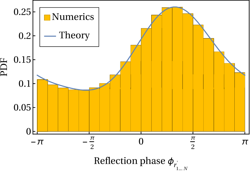
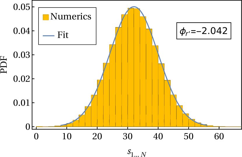
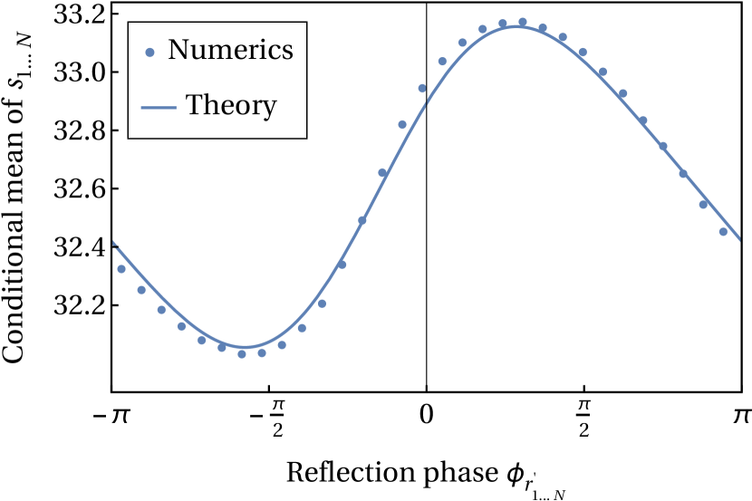
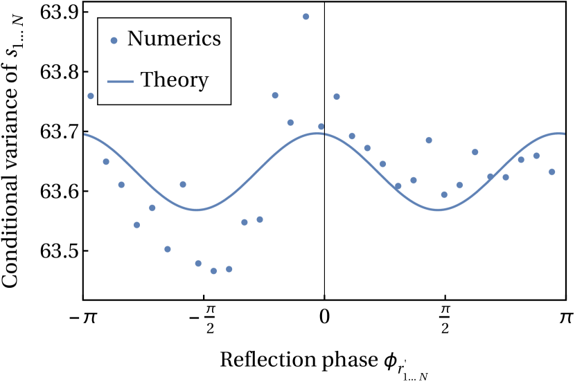
Equation (120) for the phase-dependent mean agrees well with numerics (Fig. 4c). Equation (124) for the phase-dependent variance is in rough agreement (Fig. 4d); we believe that the discrepancies could be due to a combination of (a) Eq. (124) being a leading order expression only (with the expansion parameter being ), and (b) statistical error due to having insufficiently many data points. We note that the explicit expression (124) for the phase-dependent variance is not a central part of our work, and that the numerical check of the phase-dependent mean suffices to confirm that the joint probability distribution is in general non-separable.
V Conclusion
In this paper, we developed a scattering expansion for the general problem of single-channel scattering through a disordered region with i.i.d. disorder. We found a systematic expansion of the inverse localization length and reflection phase distribution in terms of averages over the local reflection amplitudes, with the local reflection strength being the small parameter. The leading order of this expansion was shown to be equivalent to an earlier result by Schrader et al. [32], and the next order was checked in special cases from the literature. Using these first two orders, we explored the effect of phase disorder on DTQWs, interpolating between known results in the limits of weak and strong disorder and showing analytically that the localization length can vary non-monotonically in between.
In the scattering framework, we further developed the general understanding of SPS without the uniform phase hypothesis, as demonstrated by Schrader et al. [32]. In particular, we showed that their small parameter can be interpreted as the local reflection strength, and we showed that the SPS relation holds to another order beyond what they showed. We also explicitly showed that the SPS relation holds for weak potential strength in a broad class of PARS. The picture of SPS that emerges, primarily from Ref. [32] but extended by our work, is that instead of there being a length scale for complete phase randomization, there is instead a phase convergence length at which the probability distribution of the reflection phase reaches its limiting form (which in general is non-uniform). When the local reflection strength is weak and the scattering region is larger than both the localization length and the phase convergence length, SPS holds.
We proceeded to apply the scattering expansion to the joint probability distribution of the minus logarithm of the transmission coefficient () and the reflection phase (). In the limit of large system size, we obtained a general form for this distribution to all orders in the scattering expansion. This calculation relied on an ansatz and some plausible, though unproven, assumptions (and we checked our final result numerically). We showed that all quantities that appear in this general form may be expressed order by order in terms of local averages, and we explicitly evaluated some of the leading-order terms. We found that at the leading order in the local reflection strength, the same function describes both the deviations from uniformity in the marginal distribution of and the correlations between and . This showed that the joint distribution satisfies, at the leading order, a three-parameter scaling theory, with one parameter being the usual one for the SPS description of the marginal distribution of and the remaining two parameters describing both the marginal distribution of the reflection phase and the phase-transmission correlations.
It would be interesting to explore implications that our scattering-based approach might have for the more usual DTQW setup, in which a walker starts in a spatially confined initial state and evolves in time. Ballistic spread (i.e., variance increasing quadratically with time) is an important property of DTQWs and is known to be suppressed by localization. However, if the localization length is sufficiently large, then this suppression would be unimportant, since the walker can be expected to travel ballistically until reaching a distance of order . (It has indeed been found in a particular model that the maximum distance reached by the walker has the same scaling with disorder strength as the localization length [13].) Our scattering-based results for might yield a lower bound (after appropriate minimization over quasienergy) on the that appears in the time-dependent problem. Also, our technique for calculating the reflection phase distribution might extend to the distribution of the Wigner delay time (), which would characterize the time that a walker spends in being reflected from a disordered region in an otherwise non-disordered environment.
Another direction to explore would be applications of our approach to other problems involving products of random matrices, even outside the setting of scattering theory. For instance, in the study of randomly driven conformal field theories, Ref. [88] encounters a problem that seems to fit our framework [a product of random SU matrices]; each matrix represents a time step, and the Lyapunov exponent (inverse localization length) is shown to be the rate of entanglement entropy growth (and to be a lower bound on the heating rate).
Finally, this work could be a step towards an analytical treatment of the quasi-one-dimensional case (i.e., many scattering channels rather than one). This would be significant because the quasi-one-dimensional case can be used to study delocalization transitions in dimensions higher than one; in particular, one studies (usually numerically) the scaling, as the number of transverse modes goes to infinity, of the largest localization length [89]. If we can carry out the approach with multiple scattering channels, then the possibility could arise of taking this limit analytically. We note that Ref. [90] takes a similar approach in a particular model and finds that departure from the isotropy assumption (c.f. Sec. II) is necessary in order to obtain a metal-insulator transition. Ultimately, we would like to use the scattering expansion as an analytical handle on critical exponents in higher-dimensional localization-delocalization transitions, such as the plateau transition in the integer quantum Hall effect [91].
Acknowledgements.
We thank Albert Brown and Fenner Harper for collaboration on related work, and we thank Victor Gurarie, Daniel Lidar, and Abhinav Prem for discussion. A.B.C., P.S., and R.R. acknowledge financial support from the University of California Laboratory Fees Research Program funded by the UC Office of the President (UCOP), grant number LFR-20-653926. A.B.C acknowledges financial support from the Joseph P. Rudnick Prize Postdoctoral Fellowship (UCLA). P.S. acknowledges financial support from the Center for Quantum Science and Engineering Fellowship (UCLA) and the Bhaumik Graduate Fellowship (UCLA). This work used computational and storage services associated with the Hoffman2 Shared Cluster provided by UCLA Institute for Digital Research and Education’s Research Technology Group.Appendix A S matrices and scattering transfer matrices
We recall some basic facts about single-channel scattering in one dimension. A generic matrix relates incoming to outgoing scattering amplitudes by
| (125) |
and may be parametrized as
| (126) |
where and ( and ) are the transmission (reflection) amplitudes. It is straightforward to show that the unitarity condition () yields , , , and . We can thus write
| (127) |
with , , , , and (unless or ) (modulo ).
Provided that the transmission coefficient is non-zero, one can relate left to right amplitudes using a scattering transfer matrix as follows:
| (128) |
where
| (129) |
Two scatterers in sequence ( to the left of ) are described by an matrix denoted . Let us parametrize , , as in Eq. (126). may be obtained from its corresponding scattering transfer matrix . Using unitarity, it is straightforward to obtain from this matrix equation the following exact relations:
| (130a) | ||||
| (130b) | ||||
| (130c) | ||||
| (130d) | ||||
We can now derive the recursion relations for the transmission coefficient and reflection phase. Identifying , , and , we obtain Eq. (13a) from the main text by taking the modulus-squared of either Eq. (130a) or Eq. (130b). Also, we can write Eq. (130d) as
| (131) |
and taking the argument of both sides yields Eq. (13b) from the main text.
Appendix B The Schrader et al. formula
First we state the main results of Schrader et al. (Ref. [32]) with some adjustments of notation to match our conventions. Then we show that Eqs. (9) and (10) in the main text follow straightforwardly from their result.
B.1 Statement of their result
Schrader et al. consider a product of matrices , where, as in the main text, we are using the convention that the subscript stands for dependence on some disorder variables that are i.i.d. Each also depends on a global (i.e., site-independent and disorder-independent) real parameter . By assumption, each satisfies three conditions. The first is a pseudo-unitarity condition:
| (132) |
The second condition is that all commute at :
| (133) |
and the third is a trace inequality at :
| (134) |
Note that the pseudo-unitarity condition (132) with instead of is the defining condition for a scattering transfer matrix (as it is equivalent to the unitarity of the corresponding matrix). Schrader et al. point out that the two types of matrices are isomorphic, being related by a unitary transformation:
| (135) |
They write the matrix that rotates by an angle as
| (136) |
They show that any may be written as
| (137) |
where , and are real, traceless matrices, and , , , and are all independent of (while may depend on ). The phases and are explicitly found as follows. From [which follows from Eq. (132)] we have for some . The phase is defined by .
They further define a -independent constant in terms of the matrix elements of :
| (138) |
Their results for the localization length and variance [see their Eqs. (6), (7), and (22)] are given in our conventions by
| (139) |
and
| (140) |
B.2 Corollary to the Schrader et al. result
We now use the isomorphism (135) to apply Eqs. (139) and (140) to a scattering transfer matrix , which in general may be parametrized as
| (141) |
Note that by unitarity (or, equivalently, the pseudo-unitarity condition ), we have , , and . We write and . We assume that the matrix elements depend on the global parameter , and in particular that and are each proportional to . Then by unitarity, , and so
| (142) |
We expand the transmission phases as and , where the superscript indicates the order in . The scattering transfer matrix at simplifies to
| (143) |
It is then clear that all commute at . Furthermore, , which has absolute value that we can assume to be less than in almost all disorder realizations. In this last step we are appealing to “typical” disorder, since even if is enforced by symmetry, the point is a set of measure zero. The isomorphism (135) then shows that Eq. (133) and inequality (134) hold, while Eq. (132) also follows from the isomorphism. Thus, the conditions for the Schrader et al. formula are met.
We proceed to identify the various terms in the decomposition (137). From Eq. (135), we readily obtain
| (144) |
and thus
| (145) |
We then obtain .
We then define a real, traceless, -independent matrix by
| (146) |
Then it is straightforward to verify
| (147) |
which confirms the decomposition (137) with (and will not be needed).
From Eq. (138), we then read off the constant :
| (148) |
Also note
| (149a) | ||||
| (149b) | ||||
where we used the unitarity constraint . Substituting into their results (139) and (140) then yields Eqs. (9) and (10) from the main text with error terms instead of . The vanishing of the third-order contributions is discussed in the main text.
B.3 Correspondence of the phase variables
As we have mentioned in the main text, Schrader et al. [32] emphasize the importance of a non-uniform phase distribution in obtaining the correct answer for the inverse localization length and variance at leading order. To further clarify the connection between their work and ours, we show in this section that the phase variable they consider (in a calculation that does not explicitly refer to scattering) is, in the localized regime, related by a factor of to the reflection phase in our setup. We then confirm that our calculation yields the same result for the first Fourier coefficient of the phase distribution () as their calculation.
Their phase variable is (not to be confused with the coin parameter in the DTQW in our main text). Note from the paragraph above their Sec. 3 that they set ( in our notation). The recursion relation they obtain is [their Eqs. (12) and (13)]
| (150) |
where [see their Eqs. (9) and (10)]
| (151a) | ||||
| (151b) | ||||
From Eq. (145) and we see that , i.e., . Using Eq. (135) and unitarity, we then find that their recursion relation (150) becomes
| (152) |
Identifying and taking the logarithm of both sides yields exactly the recursion relation (14b) for the reflection phase in the localized regime (which we recall consists of large enough that ). This suffices to show that the probability distribution coincides with the probability distribution of for large ; while and need not coincide for small , this has no effect in the limit of many sites. Note in particular that the “invariant measure” discussed by Schrader et al. (and also in the prior mathematics literature [92, 29, 54]) is the same, up to trivial rescaling, as .
Taking in their Lemma 1 should thus yield, in our notation, the first Fourier component explicitly up to error and also the error estimate for the second Fourier component. Recall that we obtained and [see Eq. (26)], where the constants and are given by Eqs. (25b) and (25c). Recalling Eqs. (148) and (149b), we see that in the unnumbered equation above their Eq. (20) agrees with what we found for the first Fourier component (though we find a stronger error estimate). Furthermore, our explicit result for the second Fourier component is consistent with (and stronger than) their error estimate because .
Appendix C Comparison with the weak scattering approximation
Here we expand on our comments in footnotes [38, 61], providing a detailed comparison of our approach with the WSA developed in Refs. [93, 94] and reviewed in Ref. [95].
We note first that Refs. [93, 94, 95] use the convention that new scatterers are added to the left edge of the sample, rather than our convention of adding them to the right edge. The two conventions are related by exchanging and , i.e.,
| (153) |
We also note that Ref. [95] considers the special case and (see below). [Note that in this case, Eqs. (130a)–(130d) show that , but may differ from .]
With , , and , the exact recursion relations (130a)and (130d) become
| (154a) | ||||
| (154b) | ||||
where we have used a relation that follows from the unitarity constraints and :
| (155) |
Setting and and making the change of conventions given by (153), we see that Eqs. (154a) and (154b) recover the complex conjugates of the exact recursion relations as presented in Ref. [95] [Eqs. (2.16) and (2.17) there], in a slightly different notation.
We proceed next to review the WSA calculation of the inverse localization length [94]. We generalize the calculation slightly by not assuming or . We confirm that the WSA result agrees with Eq. (31) at the leading order () but disagrees at the next non-vanishing order (). Throughout, we follow the same convention as used in our main text of adding new sites to the right.
The WSA makes the following expansions of Eqs. (154a) and (154b) [95]:
| (156a) | ||||
| (156b) | ||||
[Recalling (153), we see that Eqs. (156a) and (156b) are equivalent to Eqs. (2.16) and (2.17) of Ref. [95] once we specialize to and .]. Equation (156a) is the expansion of Eq. (154a) to first order (in ). As noted below Eq. 2.19 in Ref. [95], Eq. (156b) is an uncontrolled approximation to Eq. (154b) because the first-order term is omitted (while is kept).
In the WSA approach, the inverse localization length is calculated by taking Eqs. (156a) and (156b) to be the exact recursion relations. In this way it is straightforward to obtain, by induction,
| (157) |
and
| (158) |
the latter of which recovers Eq. (13) of Ref. [94] if we set and [also recall (153)]. Then, relabeling some summation variables and using the assumption that the disorder is i.i.d., we obtain
| (159) |
The geometric sums may be carried out explicitly. Recalling that
| (160) |
and , we thus obtain
| (161) |
which indeed recovers Eq. (43) of Ref. [94] in the case and [note that the change of conventions (153) has no effect here]. Noting that and recalling Eq. (155), we then expand Eq. (161) to obtain
| (162) |
Comparing to Eq. (31) from the main text, we see that the WSA calculation yields the correct answer for at the leading order, but misses several terms that appear at the next non-vanishing order.
To compare the WSA with our work in further detail, we examine the WSA recursion relations (156a) and (156b) in the localized regime. We show that if these relations are treated consistently as first-order approximations (rather than following the WSA approach of treating them as exact), then a factor of is missing from one of the terms in the leading-order expression for the inverse localization length.
In the localized regime, becomes a pure phase (), and Eqs. (156a) and (156b) yield the following recursion relations. For the minus logarithm of the transmission coefficient, the WSA yields
| (163) |
which is indeed the leading-order expansion of Eq. (14a) from the main text. For the reflection phase, the WSA yields
| (164) |
with ; this agrees with Eq. (14b) at the zeroth order but disagrees at the first order by a constant factor ( is obtained if all first order terms are accounted for).
It is straightforward to repeat the calculation of Sec. III.2 to obtain the limiting distribution of the reflection phase at first order under the assumption of the recursion relation (164) (with as a free parameter). The result is
| (165) |
From Eq. (12), we then read off the inverse localization length at leading order:
| (166) |
which indeed agrees with Eq. (9) for (but not for ).
Appendix D Existence of the limiting distribution of the reflection phase
Given the assumption that localization occurs, we show that the probability distribution of the reflection phase, , has a limit as . The calculation here is a slight generalization of that of Lambert and Thorpe [34] with some further comments on its implications. In view of the phase correspondence discussed in Appendix B, the existence of may also be viewed as a consequence of theorems for the invariant measure [92, 29].
In the main text, we subdivided an -site sample into an -site sample plus an additional site to the right. This yielded a relation between and for large [Eq. (16)]. We now show that subdividing the -site sample in another way (an -site sample plus an additional site to the left) yields another relation between and for large , namely, the simple relation that the probability distribution stops changing as increases:
| (167) |
Equation (167) shows that exists, which in turn allows us to solve Eq. (16) (for large ) order by order in the scattering expansion, as we have done in the main text.
To obtain Eq. (167) we start by noting that, since the disorder is i.i.d., we are free to label the sites as ; in particular, we have 171717One can confirm that Eq. (168) agrees with the expression in the main text by writing the integrals over the disorder variables explicitly and then re-labeling the variables; see footnote [41].
| (168) |
With , , and , Eq. (130d) becomes
| (169) |
Assuming localization occurs, and become pure phases for large : , . Then Eq. (169) simplifies to
| (170) |
which implies that the recursion relation for the reflection phase simplifies to for large . From Eq. (168) we then read off Eq. (167).
Next, we show the connection between the calculation above and that of Lambert and Thorpe [34]. To make the precise comparison, we repeat the calculation considering the left-to-right reflection phase () instead of right-to-left reflection phase (). We write the probability distribution of as , where the superscript is only a label, and we subdivide an -site sample in the same way as in the main text (i.e., the “additional” site is on the right). From Eq. (130c) with , , and , we then obtain the analogs of Eqs. (169) and (170):
| (171a) | ||||
| (171b) | ||||
where the second equation takes to be large and uses the assumption of localization (, ). From here we can demonstrate in the same way as before [and then Eq. (167) follows by symmetry].
In a slightly more restricted setting, Eqs. (171a) and (171b) have been obtained previously in an equivalent form by Lambert and Thorpe [34], as we now explain. The restriction is the assumption that the transmission amplitudes of the local matrix are equal: . [Note that Eqs. (130a) and (130b) then imply that the sample matrix has the same property, i.e., .] Equation (171a) is then equivalent to Eq. (5c) of Ref. [34]. (To see this, we note the following correspondence between their notation and ours: , , , , , , , , and , where their quantities appear on the left-hand side and ours on the right.) Also, Eq. (171b) is stated in an equivalent form (regarding the quantity ) in the paragraph below Eq. (6) of Ref. [34].
The above calculation has a consequence for numerics, and possibly experiment, which we now explain. Sampling the reflection phase distribution could be done by finding the reflection phase in a number of different disorder realizations of a chain of fixed length; however, it may be advantageous to instead find the reflection phase for chains over a range of lengths, with no change in the disorder realization of the existing sites as new sites are added. According to the above calculation, the latter procedure will not work for sampling if the chain is increased to the right, since only a constant value of will be obtained (although our numerics indicate that can be sampled this way). Similarly, cannot be sampled by increasing the chain to the left (but we expect that can).
Appendix E Evaluation of a Fourier integral
Our series for the inverse localization length is based on Eq. (12), which we arrive at by writing the integral in Eq. (28b) as a sum over Fourier coefficients. Here we present this calculation explicitly.
Define . Since and are both real, Eq. (28b) may be written in terms of Fourier coefficients [] as
| (172) |
Thus, Eq. (12) follows from for and for , which we now show. The same Fourier integral has been done in Ref. [65] [Eq. (52) there)].
Writing , we shift to obtain
| (173) |
To show , we note that the integrand may be written as , so the integral vanishes. For , we define and (the disorder parameters represented by the site index are spectators); then we get
| (174) |
Next, we expand the logarithm to all orders in to calculate the coefficient of , which is what is the integral over yields. We get
| (175) |
from which we calculate the coefficient of to be
| (176a) | ||||
| (176b) | ||||
| (176c) | ||||
This sum evaluates to , which completes the calculation.
Appendix F Partial extension of our results to anomalies
We consider the case that the inequality (22) is only assumed for with some finite value , thus generalizing the calculation of the main text (in which ). The main conclusion of this calculation is that if is finite, then the scattering expansion that we find for in the main text is valid up to an error term . (We do not know if the odd powers are guaranteed to vanish in the case that is finite.) For instance, the leading order expression (9) is valid provided that , and the next-to-leading order expression (31) is valid provided that . We also discuss how our results for the reflection phase distribution are modified, and we present more detail for the calculation of the first few Fourier coefficients.
One motivation for doing this calculation is simply to confirm that having be large but finite, as opposed to infinite, makes no practical difference to our final results (as only very high orders are affected). A second motivation is that the case of finite arises naturally in the Anderson model for anomalous values of the momenta, as we discuss in Sec. III.3.1. (More generally, we refer to any cases in which is finite 181818To avoid cluttering the notation, we sometimes use the same symbol to refer to the maximum value of for which (22) holds for all . as “anomalies.”)
For any , we write the order- part of Eq. (17) in Fourier space:
| (177) |
Note that Eq. (19) is just Eq. (177) for . If then by assumption, so we can divide this quantity on both sides of Eq. (177) [yielding Eq. (20)].
We first prove the following statement: For any and any , the Fourier coefficients for are exactly the same as they are in the case (which is treated in the main text). Roughly speaking, this means that for large but finite , corrections to the calculation of the main text can only occur either in large frequencies or in large orders of the expansion. For example, if , then Eq. (26) is valid up to the addition of th order terms of the form (where and ).
The proof by induction is as follows. For , Eq. (177) shows that for , and also we still have by normalization; thus, agrees with the calculation for [both yielding ]. We then assume that for some , the Fourier coefficients are the same as in the case when , , and .
We consider . By normalization, . Thus, it is enough to consider with . For these , we can divide the quantity on both sides of Eq. (177). Taking without loss of generality, we then use the properties of the function that are mentioned below Eq. (24) to truncate the sum, yielding:
| (178) |
In the sum on the right-hand side, we have , , and , so each is as in the case. We can then use Eq. (23) to replace the upper limit of the sum by . We have thus arrived at an equation equivalent to Eq. (24) (since the sum there can be truncated to the same form using a property of the function ). Thus, we have shown that is as in the case, which completes the proof.
We proceed to consider the order- part (for some ) of the formula (12) for the inverse localization length. We have
| (179) |
We assume . Then in the sum on the right-hand side, which implies that each is as in the case. Thus, the inverse localization length is given by the calculation of the main text up to and including order .
We conclude this appendix by providing some further detail on the calculation of the first few Fourier coefficients [resulting in Eqs. (25a)–(25e) and (26)]. Throughout, we use the general property (which in particular holds at any given order) and the entries in Table 1.
| 0 | ||||
|---|---|---|---|---|
| 1 | ||||
| 2 | ||||
| 3 |
Setting in Eq. (24) yields . Then, setting yields , hence and . Finally, setting yields , hence , , and .
Appendix G Further details for PARS
G.1 Relation of PARS reflection amplitudes to single-site reflection amplitudes
Here we demonstrate that the scattering transfer matrix for the PARS potential (49) can be written as , where is simply related to the scattering transfer matrix for a single potential at the origin [with the reflection amplitudes in particular satisfying Eqs. (52a) and (52b)].
We start by considering the scattering problem of a single potential at the origin. A scattering eigenstate wavefunction for the Hamiltonian may be written as
| (180) |
where the energy is and where the four scattering amplitudes are related by
| (181) |
with some scattering transfer matrix that is assumed to be known.
Consider next the scattering problem for the chain defined by Eq. (49). In regions where the potential vanishes, the wavefunction is a linear combination of . We choose the following phase convention for these regions: for , we write
| (182) |
where and . By shifting , we can then refer to the single-site problem to obtain
| (183) |
Equation (182) also implies, for ,
| (184a) | ||||
| (184b) | ||||
Comparing Eq. (182) for and to Eq. (50), we also obtain
| (185) |
and
| (186) |
We define
| (187) |
Then, using the last few equations, we obtain
| (188a) | ||||
| (188b) | ||||
which confirms that the scattering transfer matrix for the sample is .
The scattering transfer matrix for the single-site problem may be parametrized as
| (189) |
and may be parametrized similarly. (In fact, by time-reversal symmetry. However, and are generally unequal unless the potential is parity symmetric.) From Eq. (187) we then read off , , and Eqs. (52a) and (52b) from the main text.
G.2 Comparison with Lambert and Thorpe
In Ref. [35], Lambert and Thorpe derive a formula for the inverse localization length to the first two non-vanishing orders in the reflection coefficient in the case of a random chain which satisfies the following properties: each scatterer has the same reflection coefficient and the phase is i.i.d. They present the case of randomly-spaced delta function potentials [in our notation, all and all ] as an example which has these properties. However, as they comment and as we now show explicitly, their result applies more generally. Here, we show that their setup applies whenever all sites have the same potential with strictly finite range and with all and all . We verify that Eq. (54) from the main text agrees with their formula.
To use their result, we set up the scattering problem with different phase conventions than we used in the main text. We write the wavefunction outside the sample as
| (190) |
while for , we write
| (191) |
where and . By shifting , we can then refer to the single-site problem [Eqs. (180) and (181)] to obtain
| (192) |
Equation (191) also implies, for ,
| (193) |
Equation (190) also implies
| (194) |
and
| (195) |
Collecting the past several equations, we obtain the scattering transfer matrix of the sample as a product of local scattering transfer matrices:
| (196) |
where and
| (197) |
From Eq. (189) we then read off , , , and .
The phase convention used above is not suitable for the setup we use in the main text because the disorder does not separate; the parameter that and depend on is not i.i.d. However, the phase convention is suitable for the setup of Lambert and Thorpe, since if we set all and take the potentials to be constant [all , hence all , all , and all ], then is indeed i.i.d. (here we have noted by unitarity). Eqs. (14)–(16), (46), and (49)–(51) of Ref. [35] then yield Eq. (54) from the main text 191919In their Eq. (51), should be .; note that our is related to their by [and see below Eq. (171b) for further details of the correspondence between our notation and theirs].
G.3 Further details for transparent mirror effect
G.3.1 Symmetry property
The scattering transfer matrix that we have used describes the scattering of a wave with momentum though a single barrier ( region). This scattering event can be decomposed into two events in sequence (as done in, e.g., Ref. [80]): first the wave passes from the region to the region with a scattering transfer matrix , then from the region to the region with scattering transfer matrix . Indeed, one obtains
| (198) |
where
| (199a) | ||||
| (199b) | ||||
For the purpose of calculating the localization length, we can just as well treat the regions at the ends ( and ) as the leads (with incoming and outgoing momentum ) and the regions as scatterers. Indeed, the scattering transfer matrix for this alternate problem may be written as
| (200) |
where
| (201) |
We assume that the disorder distributions of and are uncorrelated. Then, this alternate problem also fits into the framework of the scattering expansion: we can relabel (for ) to show explicitly that depends only on the disorder variables of site . Comparing the last several equations, we see that the scattering transfer matrix for the alternate scattering problem may be obtained by exchanging and in .
Let us now show that the alternate problem has the same localization length as the original problem. The key point is that the scattering transfer matrices for the two samples differ only by boundary terms that do not matter for large . In particular, we have
| (202) |
Note from Eq. (198) that does not depend on the disorder variables that appear in the boundary terms (i.e., and ). Thus, by a calculation similar to that in Appendix H below, we may take to show that the sample defined by a product of many has the same localization length as the sample defined by a product of many .
Finally, let us see what consequences this symmetry has on the explicit formula for as an expansion in . From the above considerations, we must get the same expansion for if we exchange and (note that this includes exchanging the disorder distributions of the and variables) in Eqs. (60b) and (61). As discussed in the main text, we leave momenta and as they are [i.e., not expanding in using Eq. (59b)] when they appear in trigonometric functions. This leaves the terms and as the only ones that will be expanded in . The latter of these is invariant under . The former is odd, but this change of sign always cancels because and must appear in the same number of powers in each term of the expansion of (as we recall from the symmetry argument in Sec. III.1). Thus, the expansion of in powers of must be symmetric under the exchange of and at each order (with the understanding that is unaffected by the exchange).
G.3.2 Comparison with the literature
We compare our results with Refs. [80, 82, 81], starting with Ref. [80]. Although this reference focuses on the case that disorder is strong in both and , an intermediate result is presented there that is valid for strong disorder in and arbitrary disorder in . In our notation, the unnumbered equation above their Eq. (32) is equivalent to
| (203a) | ||||
| (203b) | ||||
where is the index of refraction and where we have used Eqs. (59a) and (59b). From (61), we see that the above equation is another way of writing the uniform phase result, i.e., .
Next, we verify that Eq. (62) from the main text agrees with Eq. (5.14) from Ref. [82] in the regime in which the two calculations overlap. Ref. [82] considers the case of weak disorder in and no disorder in , with treated without approximation. To convert their notation to ours and expand their result in , we set , and , where their quantities appear on the left and ours on the right. Thus, their Eq. (5.14) has the following expansion in :
| (204) |
where is the variance of about its average. We indeed recover this answer from Eq. (62) by expanding in weak disorder in [c.f. also the comment below Eq. (57) about restoring dimensions].
Finally, we compare Eq. (62) to a result from [81], apparently finding some differences in numerical factors. This reference considers and to follow exponential distributions:
| (205) |
where and here are site-independent constants. With these disorder distributions, Eq. (62) yields
| (206) |
in which we have expanded in and restored physical dimensions. To compare with the last unnumbered equation on page 400 of Ref. [81], we use the following conversion from their notation to ours. They present the logarithm of the average of the transmission, rather than the average of the logarithm; thus, their result is [defined in their Eq. (29.19)]. By their Eqs. (30.34)–(30.36), our is the same quantity as their . We have , and [c.f. their page 76 and Eqs. (29.1) and (29.21); note in particular that they set the mass ], where their quantities appear on the left and ours on the right. All together, their result seems to yield Eq. (206) with the factors of and on the right-hand side both absent.
We note that Eq. (206) (regardless of whether or not the and are included) is monotonic in disorder strength (i.e., either or is varied) if the localization length is expressed in units of the average lattice spacing, that is, if the factor is removed. If instead this factor is included, then non-monotonicity is obtained.
Appendix H Tarasinski leads and their equivalence to other leads
Let us first fill in the details for the calculation of the transfer matrix [18]. Writing a general state as one finds that the stationary state equation is equivalent to the following pair of equations:
| (207a) | |||
| (207b) | |||
which are Eqs. (11) and (12) of Ref. [18] with 202020We correct sign errors in Eqs. (11) and (12) of Ref. [18] (the sign of the second term on the right-hand side of each equation). Rearranging these yields the transfer matrix [Eq. (68) from the main text].
We proceed to set up the scattering problem with Tarasinski leads, which we recall are defined by setting for and for . Note that for these , the transfer matrix simplifies to
| (208) |
The solutions in the leads are therefore linear combinations of and , with quasienergy . A scattering solution may then be parametrized outside the sample as
| (209) |
which is Eq. (69) from the main text (written in a form that we generalize below).
To set up the scattering problem with other choices of leads, we next recall the solution in the clean case, i.e., , , , and . Here we follow Ref. [18], correcting some sign errors there. Writing a Bloch wave solution as for some two-component Bloch “spinor” , we find that Eqs. (207a) and (207b) become
| (210) |
Thus, the clean quasienergy spectrum is determined by 212121This corrects a sign error in Eq. (6) of Ref. [18] ().
| (211) |
and the Bloch spinors are determined up to overall phase and normalization by 222222This corrects a sign error in Eq. (7) of Ref. [18] (). Note that Eq. (7) there is derived using the convention , which accounts for the extra factor of in our equation ().
| (212) |
See Fig. 2 of Ref. [18] for the quasienergy spectrum at various values of .
We can now consider a scattering state with quasienergy in the problem with for and for . At any (aside from exceptional points) there are two corresponding momenta in the first Brillouin zone [c.f. Eq. (211)]. One momentum is right moving and the other left moving; we label them as and , respectively. (Explicitly, the group velocity is positive at and negative at .) A scattering solution may be written outside the sample as
| (213) |
Note that Eq. (209) is a special case with (assuming ) , , and .
To bring this scattering problem to the form to which our setup applies, we define (as in Sec. III.3.1) a matrix that converts position-space amplitudes to scattering amplitudes:
| (214) |
Then
| (215) |
Multiplying transfer matrices then yields
| (216) |
where
| (217) |
is the scattering transfer matrix for the sample in this setup. We then read off .
While we could now apply our results to the problem with these more general leads, it is more convenient to instead show that the probability distribution of the minus logarithm of the transmission coefficient is the same for all choices of leads. To do this, let us write the sample transmission coefficient as for the problem with Tarasinski leads and as for the problem with more general leads. Our goal is to show that for large samples, and have the same probability distribution.
The claim follows immediately from the relation
| (218) |
in which the only difference between the two scattering transfer matrices is multiplication by boundary terms, which have negligible effect as . To see this explicitly, we parametrize in terms of the transmission coefficient and transmission and reflection phases, and then we expand in small :
| (219a) | ||||
| (219b) | ||||
By the assumption that localization occurs, the error term is exponentially small for large . Eq. (218) [with also expanded as in Eq. (219b)] then yields
| (220) |
in which the second, third, and fourth terms on the right-hand side are all as (all may be bounded by -independent constants). The omitted terms are exponentially small in . Thus, we confirm that and are asymptotically equal, and hence they have the same probability distribution.
Appendix I Toy recursion relation
To help illustrate our calculation of the joint probability distribution, we apply the same method to a toy example: a random walk with variable step lengths. This example will also explain the comment below Eq. (96) regarding the convenience of working with a variable that does not increase on average.
Consider a toy recursion relation given by
| (221) |
where the random variables are i.i.d. and where some initial value is given. For large the probability distribution of [] goes to a Gaussian with mean and variance . We proceed next to recover this result by applying the approach we used in Sec. IV.
We start by defining a shifted variable , where is any constant. The recursion relation for is readily found to be , from which we obtain the recursion relation for the probability distribution of []
| (222a) | ||||
| (222b) | ||||
where we note that is a linear functional in its last argument. To solve this equation, we will make an ansatz that is proportional to and show
| (223) |
Our ansatz is a Gaussian with mean and variance that both scale linearly with , i.e.,
| (224) |
where and are constants to be determined by requiring Eq. (223) to hold. Equation (223) will also hold if the mean and variance in the ansatz have arbitrary -independent constants added; in the terminology of Sec. IV.2, these constants parametrize a family of trajectories that satisfy the recursion relation up to small error.
Converting to Fourier space, we obtain
| (225a) | ||||
| (225b) | ||||
and
| (226) |
The error estimate (110) from the main text, with replaced by , still holds because the constant only appears in the overall phase. Thus, we can neglect terms of the form (with ) in , since they are in space.
We next do a Taylor expansion of in . Unless the constant is zero (as in the main text), we must include the second derivative term in this expansion; the key relation is
| (227a) | ||||
| (227b) | ||||
from which Eq. (225b) yields
| (228) |
Thus, requiring Eq. (223) to hold for large uniquely determines the constants and :
| (229a) | ||||
| (229b) | ||||
which are the correct values. Note that if we choose , then we need not include the second derivative term in Eq. (227a), since ; this is essentially what is done in the main text.
In contrast, we show next that a naive calculation based on finding a Fokker-Planck equation for yields the variance of depending on , which is incorrect unless a particular value of is chosen.
Starting from the recursion relation (222a), we consider to be a small parameter [more precisely, we replace and expand in ]. Expanding the delta function on the right-hand side yields
| (230) |
Taking large we replace (although this step turns out not to be correct in general)
| (231) |
and we thus obtain the Fokker-Planck equation:
| (232) |
The initial condition does not affect the slope in of the mean or variance, but for definiteness let us take so that and hence . Then the solution of Eq. (232) (dropping the third-order error term) is the Gaussian with mean and variance . Shifting back to the original variable , we see that the mean is correct, but the variance is wrong unless we choose .
The problem with the calculation just presented is that the expansion (231) needs to be done to one more order, as in Eqs. (227a) and (227b). In other words, it is turns out that the solution Eq. (232) is such that the replacement (231) is not consistent (in that the second derivative term is not in fact negligible). If is chosen, then , so the second derivative term in (227b) vanishes and the replacement (231) is correct.
References
- Abrahams [2010] E. Abrahams, ed., 50 Years of Anderson Localization (World Scientific, Singapore, 2010).
- Childs [2009] A. M. Childs, Universal Computation by Quantum Walk, Physical Review Letters 102, 180501 (2009).
- Lovett et al. [2010] N. B. Lovett, S. Cooper, M. Everitt, M. Trevers, and V. Kendon, Universal quantum computation using the discrete-time quantum walk, Physical Review A 81, 042330 (2010).
- Singh et al. [2021] S. Singh, P. Chawla, A. Sarkar, and C. M. Chandrashekar, Universal quantum computing using single-particle discrete-time quantum walk, Scientific Reports 11, 11551 (2021).
- Kempe [2003] J. Kempe, Quantum random walks: An introductory overview, Contemporary Physics 44, 307 (2003).
- Venegas-Andraca [2012] S. E. Venegas-Andraca, Quantum walks: A comprehensive review, Quantum Information Processing 11, 1015 (2012).
- Kadian et al. [2021] K. Kadian, S. Garhwal, and A. Kumar, Quantum walk and its application domains: A systematic review, Computer Science Review 41, 100419 (2021).
- Perets et al. [2008] H. B. Perets, Y. Lahini, F. Pozzi, M. Sorel, R. Morandotti, and Y. Silberberg, Realization of Quantum Walks with Negligible Decoherence in Waveguide Lattices, Physical Review Letters 100, 170506 (2008).
- Schreiber et al. [2011] A. Schreiber, K. N. Cassemiro, V. Potoček, A. Gábris, I. Jex, and C. Silberhorn, Decoherence and Disorder in Quantum Walks: From Ballistic Spread to Localization, Physical Review Letters 106, 180403 (2011).
- Crespi et al. [2013] A. Crespi, R. Osellame, R. Ramponi, V. Giovannetti, R. Fazio, L. Sansoni, F. De Nicola, F. Sciarrino, and P. Mataloni, Anderson localization of entangled photons in an integrated quantum walk, Nature Photonics 7, 322 (2013).
- Vatnik et al. [2017] I. D. Vatnik, A. Tikan, G. Onishchukov, D. V. Churkin, and A. A. Sukhorukov, Anderson localization in synthetic photonic lattices, Scientific Reports 7, 4301 (2017).
- Törmä et al. [2002] P. Törmä, I. Jex, and W. P. Schleich, Localization and diffusion in Ising-type quantum networks, Physical Review A 65, 052110 (2002).
- Keating et al. [2007] J. P. Keating, N. Linden, J. C. F. Matthews, and A. Winter, Localization and its consequences for quantum walk algorithms and quantum communication, Physical Review A 76, 012315 (2007).
- Yin et al. [2008] Y. Yin, D. E. Katsanos, and S. N. Evangelou, Quantum walks on a random environment, Physical Review A 77, 022302 (2008).
- Joye and Merkli [2010] A. Joye and M. Merkli, Dynamical Localization of Quantum Walks in Random Environments, Journal of Statistical Physics 140, 1025 (2010).
- Ahlbrecht et al. [2011] A. Ahlbrecht, V. B. Scholz, and A. H. Werner, Disordered quantum walks in one lattice dimension, Journal of Mathematical Physics 52, 102201 (2011).
- Obuse and Kawakami [2011] H. Obuse and N. Kawakami, Topological phases and delocalization of quantum walks in random environments, Physical Review B 84, 195139 (2011).
- Vakulchyk et al. [2017] I. Vakulchyk, M. V. Fistul, P. Qin, and S. Flach, Anderson localization in generalized discrete-time quantum walks, Physical Review B 96, 144204 (2017).
- Derevyanko [2018] S. Derevyanko, Anderson localization of a one-dimensional quantum walker, Scientific Reports 8, 1795 (2018).
- Chandrashekar and Busch [2015] C. M. Chandrashekar and T. Busch, Localized quantum walks as secured quantum memory, EPL (Europhysics Letters) 110, 10005 (2015).
- Note [0] For clarification on how a wave interference effect such as Anderson localization (i.e., an effect not uniquely quantum) can be relevant to quantum computing, see Refs. [102, 103, 104, 105].
- Chandrashekar et al. [2008] C. M. Chandrashekar, R. Srikanth, and R. Laflamme, Optimizing the discrete time quantum walk using a SU(2) coin, Physical Review A 77, 032326 (2008).
- Chandrashekar et al. [2010] C. M. Chandrashekar, R. Srikanth, and R. Laflamme, Erratum: Optimizing the discrete time quantum walk using a SU(2) coin [Phys. Rev. A 77, 032326 (2008)], Physical Review A 82, 019902(E) (2010).
- Abrahams et al. [1979] E. Abrahams, P. W. Anderson, D. C. Licciardello, and T. V. Ramakrishnan, Scaling Theory of Localization: Absence of Quantum Diffusion in Two Dimensions, Physical Review Letters 42, 673 (1979).
- Shapiro [1987] B. Shapiro, Scaling properties of probability distributions in disordered systems, Philosophical Magazine B 56, 1031 (1987).
- Cohen et al. [1988] A. Cohen, Y. Roth, and B. Shapiro, Universal distributions and scaling in disordered systems, Physical Review B 38, 12125 (1988).
- Anderson et al. [1980] P. W. Anderson, D. J. Thouless, E. Abrahams, and D. S. Fisher, New method for a scaling theory of localization, Physical Review B 22, 3519 (1980).
- Note [1] To be precise, we are considering here the two-terminal conductance rather than the four-terminal conductance [106], where is the reflection coefficient of the sample; however, the distinction does not matter in the localized regime (in which ) that is our focus throughout. Also, we are ignoring spin degeneracy. In the rest of the paper, we set .
- Bougerol and Lacroix [1985] P. Bougerol and J. Lacroix, eds., Products of Random Matrices with Applications to Schrödinger Operators (Birkhäuser Boston, Boston, MA, 1985).
- Deych et al. [2000] L. I. Deych, A. A. Lisyansky, and B. L. Altshuler, Single Parameter Scaling in One-Dimensional Localization Revisited, Physical Review Letters 84, 2678 (2000).
- Deych et al. [2001] L. I. Deych, A. A. Lisyansky, and B. L. Altshuler, Single-parameter scaling in one-dimensional Anderson localization: Exact analytical solution, Physical Review B 64, 224202 (2001).
- Schrader et al. [2004] R. Schrader, H. Schulz-Baldes, and A. Sedrakyan, Perturbative Test of Single Parameter Scaling for 1D Random Media, Annales Henri Poincaré 5, 1159 (2004).
- Tarasinski et al. [2014] B. Tarasinski, J. K. Asbóth, and J. P. Dahlhaus, Scattering theory of topological phases in discrete-time quantum walks, Physical Review A 89, 042327 (2014).
- Lambert and Thorpe [1982] C. J. Lambert and M. F. Thorpe, Phase averaging in one-dimensional random systems, Physical Review B 26, 4742 (1982).
- Lambert and Thorpe [1983] C. J. Lambert and M. F. Thorpe, Random $T$-matrix approach to one-dimensional localization, Physical Review B 27, 715 (1983).
- Barkhofen et al. [2017] S. Barkhofen, T. Nitsche, F. Elster, L. Lorz, A. Gábris, I. Jex, and C. Silberhorn, Measuring topological invariants in disordered discrete-time quantum walks, Physical Review A 96, 033846 (2017).
- Culver et al. [2024] A. B. Culver, P. Sathe, and R. Roy, Scattering expansion for localization in one dimension, Physical Review B 109, L060201 (2024).
- Note [2] As we comment on in the main body of this paper and in Appendix B, some of the results of our expansion at leading order were obtained in an equivalent form by Schrader et al. in Ref. [32] (see also Ref. [53]). Also, in the context of light propagation in disordered metamaterials, a similar expansion called the weak scattering approximation (WSA) was done in Refs. [93, 94] (see [95] for a review); however, the WSA has an uncontrolled aspect that is not present in our work (see Appendix C).
- Deych et al. [1998] L. I. Deych, D. Zaslavsky, and A. A. Lisyansky, Statistics of the Lyapunov Exponent in 1D Random Periodic-on-Average Systems, Physical Review Letters 81, 5390 (1998).
- Note [3] Non-monotonicity in disorder strength has been found previously, both analytically and numerically, in particular PARS problems [35, 83] (see Sec. III.3.2). Also, it has been shown that transmission through a disordered region can be non-monotonic in disorder strength when the incident wave is in an energy gap of the non-disordered system (see Ref. [107] and references therein); we do not consider this case.
- Note [4] Explicitly, we have (e.g.) , where . Due to the disorder being i.i.d., the probability distributions depend only on the number of consecutive sites and not on their location. Also, to make contact with the notation used in the Introduction, we take the spacing between sites to be the unit of distance; then the length of the sample is .
- Vagner et al. [2003] P. Vagner, P. Markoš, M. Moško, and T. Schäpers, Coherent resistance of a disordered one-dimensional wire: Expressions for all moments and evidence for non-Gaussian distribution, Physical Review B 67, 165316 (2003).
- Pendry [1994] J. Pendry, Symmetry and transport of waves in one-dimensional disordered systems, Advances in Physics 43, 461 (1994).
- Jayannavar [1990] A. M. Jayannavar, Phase distribution of an electronic wave function in a random medium, Solid State Communications 73, 247 (1990).
- Jayannavar [1991] A. M. Jayannavar, Scaling theory of quantum resistance distributions in disordered systems, Pramana 36, 611 (1991).
- Heinrichs [2002] J. Heinrichs, Relation between Anderson and invariant imbedding models for transport in finite chains and study of phase and delay time distributions for strong disorder, Physical Review B 65, 075112 (2002).
- Pradhan [2021] P. Pradhan, Phase Statistics of Light/Photonic Wave Reflected from One-Dimensional Optical Disordered Media and Its Effects on Light Transport Properties, Photonics 8, 485 (2021).
- Dorokhov [1982] O. N. Dorokhov, Localization and transmission coefficient for two coupled metal chains with disorder, Solid State Communications 44, 915 (1982).
- Schomerus and Titov [2003] H. Schomerus and M. Titov, Band-center anomaly of the conductance distribution in one-dimensional Anderson localization, Physical Review B 67, 100201(R) (2003).
- Tessieri and Izrailev [2018] L. Tessieri and F. M. Izrailev, Anomalies in the 1D Anderson model: Beyond the band-centre and band-edge cases, Physica E: Low-dimensional Systems and Nanostructures 97, 401 (2018).
- Lambert et al. [1983] C. J. Lambert, P. D. Beale, and M. F. Thorpe, Phase recurrences and metastability in a one-dimensional solid, Physical Review B 27, 5860 (1983).
- Stone et al. [1983] A. D. Stone, D. C. Allan, and J. D. Joannopoulos, Phase randomness in the one-dimensional Anderson model, Physical Review B 27, 836 (1983).
- Drabkin and Schulz-Baldes [2015] M. Drabkin and H. Schulz-Baldes, Gaussian fluctuations of products of random matrices distributed close to the identity, Journal of Difference Equations and Applications 21, 467 (2015).
- Jitomirskaya et al. [2003] S. Jitomirskaya, H. Schulz-Baldes, and G. Stolz, Delocalization in Random Polymer Models, Communications in Mathematical Physics 233, 27 (2003).
- Mello [1987] P. A. Mello, Macroscopic approach to the theory of one-dimensional disordered conductors, Physical Review B 35, 1082 (1987).
- Note [5] Reference [55] obtains a Fokker-Planck equation for the probability distribution of . In the localized regime that is our focus, Ref. [55] uses this Fokker-Planck equation to obtain a Gaussian distribution for (there denoted ), as we have stated in the main text. The phase variables in Ref. [55], which are distributed uniformly [c.f. Eq. (2.6) there)], are related to the reflection phases by and [c.f. Eqs. (2.3a) and (2.3b) there].
- Mello et al. [1988] P. A. Mello, P. Pereyra, and N. Kumar, Macroscopic approach to multichannel disordered conductors, Annals of Physics 181, 290 (1988).
- Mello and Pichard [1991] P. A. Mello and J.-L. Pichard, Symmetries and parametrization of the transfer matrix in electronic quantum transport theory, Journal de Physique I 1, 493 (1991).
- Xie et al. [2012] H.-Y. Xie, V. E. Kravtsov, and M. Müller, Anderson localization of one-dimensional hybrid particles, Physical Review B 86, 014205 (2012).
- Roberts [1992] P. J. Roberts, Joint probability distributions for disordered 1D wires, Journal of Physics: Condensed Matter 4, 7795 (1992).
- Note [6] In the case of and , a result related to Eq. (9\@@italiccorr) has also been obtained in Refs. [93, 94, 95] using the WSA approach developed there. See Appendix C for details.
- Note [7] In the particular case of the Anderson model with onsite disorder with vanishing mean, Ref. [32] calculates the third and fourth order terms and finds that the third order terms indeed vanish.
- Note [8] Whenever we require a property to hold for all disorder realizations, we expect that it would also suffice for that property to hold for almost all realizations (i.e., all except a set of measure zero).
- Note [9] A similar point is mentioned in Ref. [26] (footnote 24).
- Rauh [2009] A. Rauh, Analytical Localization Lengths in an One-Dimensional Disordered Electron System, Zeitschrift für Naturforschung A 64, 205 (2009).
- Sulem [1973] P. L. Sulem, Total reflection of a plane wave from a semi-infinite, one-dimensional random medium: Distribution of the phase, Physica 70, 190 (1973).
- Note [10] See, e.g., the second unnumbered equation below Eq. (36) in Ref. [32] (which cites earlier work). Our Appendix B provides some details for converting the notation of Ref. [32] into our notation.
- Feng et al. [2019] D. Feng, Y. Cui, K. Kang, S. Qin, and C. Wang, Localization behavior induced by asymmetric disorder for the one-dimensional Anderson model, Physical Review E 100, 042102 (2019).
- Abrahams and Stephen [1980] E. Abrahams and M. J. Stephen, Resistance fluctuations in disordered one-dimensional conductors, Journal of Physics C: Solid State Physics 13, L377 (1980).
- Barnes and Luck [1990] C. Barnes and J. M. Luck, The distribution of the reflection phase of disordered conductors, Journal of Physics A: Mathematical and General 23, 1717 (1990).
- Note [11] Here we explain the comparison with Refs. [70] and [60] in more detail. From Eq. (4.21) of Ref. [70], we see that the coefficients there are related to our notation by . We specialize to the symmetric exponential distribution with width by setting , yielding agreement with Eq. (4.23) there. To compare with Ref. [60], we note from Eq. (54) there that in our notation, and we integrate over in Eq. (55) there to obtain , i.e., the distribution of . By Eq. (42\@@italiccorr), we have , resulting in the sign discrepancy mentioned in the main text.
- Lambert [1984] C. J. Lambert, Anomalies in the transport properties of a disordered solid, Physical Review B 29, 1091 (1984).
- Derrida and Gardner [1984] B. Derrida and E. Gardner, Lyapounov exponent of the one dimensional Anderson model : Weak disorder expansions, Journal de Physique 45, 1283 (1984).
- Bovier and Klein [1988] A. Bovier and A. Klein, Weak disorder expansion of the invariant measure for the one-dimensional Anderson model, Journal of Statistical Physics 51, 501 (1988).
- Kappus and Wegner [1981] M. Kappus and F. Wegner, Anomaly in the band centre of the one-dimensional Anderson model, Zeitschrift für Physik B Condensed Matter 45, 15 (1981).
- Note [12] We can expect our results to hold also if the potentials are sufficiently small (e.g., exponentially decaying) for .
- Note [13] This model provides an example of correlations between the parameters of , which are allowed in our setup. In particular, the parameters of the square well potential are first promoted to site-dependent parameters . We then set all and ; in , the potential width is thus correlated with the width .
- Izrailev et al. [2012] F. M. Izrailev, A. A. Krokhin, and N. M. Makarov, Anomalous localization in low-dimensional systems with correlated disorder, Physics Reports Anomalous Localization in Low-Dimensional Systems with Correlated Disorder, 512, 125 (2012).
- Note [14] For a definite counterexample, consider , i.e., an array of delta function potentials with random strengths. If , then Eq. (6\@@italiccorr) is not correct at leading order in weak disorder, even if .
- Berry and Klein [1997] M. V. Berry and S. Klein, Transparent mirrors: Rays, waves and localization, European Journal of Physics 18, 222 (1997).
- Lifshits et al. [1988] I. M. Lifshits, S. A. Gredeskul, and L. A. Pastur, Introduction to the Theory of Disordered Systems (Wiley, 1988).
- Luna-Acosta et al. [2009] G. A. Luna-Acosta, F. M. Izrailev, N. M. Makarov, U. Kuhl, and H.-J. Stöckmann, One dimensional Kronig-Penney model with positional disorder: Theory versus experiment, Physical Review B 80, 115112 (2009).
- Mafi [2015] A. Mafi, Anderson localization in a partially random Bragg grating and a conserved area theorem, Optics Letters 40, 3603 (2015).
- Upadhyaya and Amir [2018] N. Upadhyaya and A. Amir, Disorder engineering: From structural coloration to acoustic filters, Physical Review Materials 2, 075201 (2018).
- Joy et al. [2020] S. Joy, S. Khalid, and B. Skinner, Transparent mirror effect in twist-angle-disordered bilayer graphene, Physical Review Research 2, 043416 (2020).
- Note [15] In the special case of weak disorder in , Ref. [18] mentions a factor of discrepancy between their analytical and numerical results for [see below their Eq. (29)], and it is in the right direction to agree with our result. We believe that this factor of is also present in their analytical calculations for weak disorder in or in , as removing it restores agreement with our results in those cases as well. The factor of that appears in our convention of presenting the localization length in the form has been accounted for in this discussion and is not the source of the discrepancy.
- Note [16] See Eq. (11) of Ref. [19], where is our and is our .
- Wen et al. [2022] X. Wen, Y. Gu, A. Vishwanath, and R. Fan, Periodically, Quasi-periodically, and Randomly Driven Conformal Field Theories (II): Furstenberg’s Theorem and Exceptions to Heating Phases, SciPost Physics 13, 082 (2022).
- Römer [2022] R. A. Römer, Numerical methods for localization, in Reference Module in Materials Science and Materials Engineering (Elsevier, 2022).
- Chalker and Bernhardt [1993] J. T. Chalker and M. Bernhardt, Scattering theory, transfer matrices, and Anderson localization, Physical Review Letters 70, 982 (1993).
- Chalker and Coddington [1988] J. T. Chalker and P. D. Coddington, Percolation, quantum tunnelling and the integer Hall effect, Journal of Physics C: Solid State Physics 21, 2665 (1988).
- Furstenberg [1963] H. Furstenberg, Noncommuting random products, Transactions of the American Mathematical Society 108, 377 (1963).
- Asatryan et al. [2007] A. A. Asatryan, L. C. Botten, M. A. Byrne, V. D. Freilikher, S. A. Gredeskul, I. V. Shadrivov, R. C. McPhedran, and Y. S. Kivshar, Suppression of Anderson Localization in Disordered Metamaterials, Physical Review Letters 99, 193902 (2007).
- Asatryan et al. [2010] A. A. Asatryan, S. A. Gredeskul, L. C. Botten, M. A. Byrne, V. D. Freilikher, I. V. Shadrivov, R. C. McPhedran, and Y. S. Kivshar, Anderson localization of classical waves in weakly scattering metamaterials, Physical Review B 81, 075124 (2010).
- Gredeskul et al. [2012] S. A. Gredeskul, Y. S. Kivshar, A. A. Asatryan, K. Y. Bliokh, Y. P. Bliokh, V. D. Freilikher, and I. V. Shadrivov, Anderson localization in metamaterials and other complex media (Review Article), Low Temperature Physics 38, 570 (2012).
- Note [17] One can confirm that Eq. (168\@@italiccorr) agrees with the expression in the main text by writing the integrals over the disorder variables explicitly and then re-labeling the variables; see footnote [41].
- Note [18] To avoid cluttering the notation, we sometimes use the same symbol to refer to the maximum value of for which (22\@@italiccorr) holds for all .
- Note [19] In their Eq. (51), should be .
- Note [20] We correct sign errors in Eqs. (11) and (12) of Ref. [18] (the sign of the second term on the right-hand side of each equation).
- Note [21] This corrects a sign error in Eq. (6) of Ref. [18] ().
- Note [22] This corrects a sign error in Eq. (7) of Ref. [18] (). Note that Eq. (7) there is derived using the convention , which accounts for the extra factor of in our equation ().
- Lloyd [1999] S. Lloyd, Quantum search without entanglement, Physical Review A 61, 010301(R) (1999).
- Bhattacharya et al. [2002] N. Bhattacharya, H. B. van Linden van den Heuvell, and R. J. C. Spreeuw, Implementation of Quantum Search Algorithm using Classical Fourier Optics, Physical Review Letters 88, 137901 (2002).
- Knight et al. [2003] P. L. Knight, E. Roldán, and J. E. Sipe, Quantum walk on the line as an interference phenomenon, Physical Review A 68, 020301(R) (2003).
- Perez-Garcia et al. [2015] B. Perez-Garcia, J. Francis, M. McLaren, R. I. Hernandez-Aranda, A. Forbes, and T. Konrad, Quantum computation with classical light: The Deutsch Algorithm, Physics Letters A 379, 1675 (2015).
- Datta [1995] S. Datta, Electronic Transport in Mesoscopic Systems, Cambridge Studies in Semiconductor Physics and Microelectronic Engineering (Cambridge University Press, Cambridge, 1995).
- Heinrichs [2008] J. Heinrichs, Enhanced quantum tunnelling induced by disorder, Journal of Physics: Condensed Matter 20, 395215 (2008).