Scheduling Algorithms for Hierarchical Fog Networks
Abstract
Fog computing brings the functionality of the cloud near the edge of the network with the help of fog devices/micro data centers (mdcs). Job scheduling in such systems is a complex problem due to the hierarchical and geo-distributed nature of fog devices. We propose two fog scheduling algorithms, named FiFSA (Hierarchical First Fog Scheduling Algorithm) and EFSA ( Hierarchical Elected Fog Scheduling Algorithm). We consider a hierarchical model of fog devices, where the computation power of fog devices present in higher tiers is greater than those present in lower tiers. However, the higher tier fog devices are located at greater physical distance from data generation sources as compared to lower tier fog devices. Jobs with varying granularity and cpu requirements have been considered. In general, jobs with modest cpu requirements are scheduled on lower tier fog devices, and jobs with larger cpu requirements are scheduled on higher tier fog devices or the cloud data center (cdc). The performance of FiFSA and EFSA has been evaluated using a real life workload trace on various simulated fog hierarchies as well as on a prototype testbed. Employing FiFSA offers an average improvement of 27% and 57.9% in total completion time and an improvement of 32% and 61% in cost as compared to Longest Time First (LTF) and cloud-only (cdc-only) scheduling algorithms, respectively. Employing EFSA offers an average improvement of 48% and 70% in total completion time and an improvement of 52% and 72% in cost as compared to LTF and cdc-only respectively.
Index Terms:
fog computing, cloud computing, fog device hierarchyI Introduction
The evolution of IoT devices has lead to the generation of huge amounts of data which needs to be monitored, processed, and analysed [32]. Due to ample computation power and storage volume, the cloud has become a competent model to execute user applications [7]. The cloud data center is used to process the application data, which is managed by cloud service providers, such as Amazon, Google, or Microsoft Azure. A significant delay in processing the applications has been observed at the cloud data center, owing to its distant geographic location from the users. This delay may be unacceptable for applications with stringent response times, such as smart healthcare [11]. To overcome this delay constraint, system designers are exploring fog computing [13, 38].
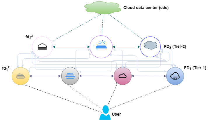
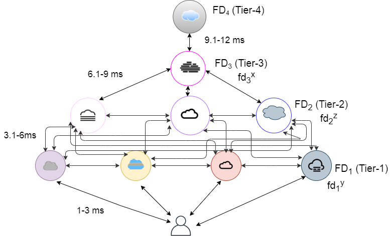
In general, a cloud only architecture may not be suitable for latency sensitive applications, due to the distance issue highlighted above. Fog computing offers an architecture comprising of a number of fog devices/micro data centres, in close proximity to data generation sources, such as smartphones and sensors. Hence, the generated data can be processed on the fog devices in a timely manner. It has been observed that fog devices have limited computation power and storage capacity [10]. Hence, they are able to handle jobs with modest cpu requirements, e.g. interactive jobs. Therefore, a flat fog only architecture may not be suitable for processing jobs with less modest execution requirements. This seems to suggest a hierarchical fog-cloud architecture, consisting of multiple fog-tiers and a cloud data center. Accordingly, we consider a hierarchy of fog devices in our architecture [24]. As an example, consider a 2-tier fog-cloud hierarchy, where tier-1 fog devices have a lower execution capacity than tier-2 fog devices. On the flip side, tier-2 fog devices are located at a greater geographical distance than tier-1 fog devices from the users. Thus, there exists an interesting trade off between execution capacity and propagation delay of tier-1 and tier-2 fog nodes. The proposed architecture is depicted in Fig.1. Note that this model can be extended to accommodate a larger number of fog tiers, based on application requirements.
As a use case to drive the proposed algorithms, let us discuss a “smart home”. Typically, a smart home uses various internet connected devices that allows monitoring and supervision. Due to the large number of these devices, such smart homes will generate huge amounts of data per hour. As per the computer business review [25], it has been reported that UK smart households will generate 26 million GBs of data every week. Some of this data may need real-time responses. Due to network congestion and delayed response times, the cloud data center may not be a suitable option for processing such time-critical data. Handling some of this data at the nearby fog layer may assure real-time response times to users. A smart home scenario can involve a number of sensors, such as: motion sensors, water sensors, temperature sensors, light sensors, weather sensors etc. A smart home uses the data provided by these sensors to perform various functions such as warning for gas leaks, emergency health services, maintaining the thermostat, managing lights, maintaining the laundry cycle of the washing machine, domestic grocery shopping based on shopping history etc. These jobs will have diverse execution requirements. An example of a job with relatively modest cpu requirements is activating a burglar alarm or a fire detection system. If the alarm isn’t generated quickly, then there is a possibility of theft or causalities. It may not be wise to process such data at the cloud data center, due to the significant latency involved. Such jobs should be sent to tier-1 fog devices located in proximity to the user. On the other hand, jobs with medium cpu requirements could be related to maintaining the comfort of the home, such as roller shutter automation, maintaining air-conditioning, switching lights on/off etc. These are examples of jobs with moderate cpu requirements that may be executed at tier-2 fog devices. Lastly, the jobs with high cpu requirements can be executed at the cloud data center. Examples of these jobs could be automatically recording TV programs for subsequent viewing of users. Besides offering reduced response times for job execution, another advantage of fog devices is that they are geographically distributed without a single point of failure, so the service may not be disrupted in the case of device failure.
The main contributions of this paper can be summarised as :
-
•
We propose scheduling algorithms for hierarchical fog-cloud architectures with multiple layers of fog devices between the users and the cloud data center. Specifically, we consider flat-tier, 2-tier, 3-tier and 4-tier fog architectures. We formulate our research problem by jointly minimising the completion time as well as the energy consumption on an n-tiered fog-cloud architecture.
-
•
In order to minimise the completion times of the jobs, we propose two hierarchical scheduling algorithms: FiFSA (Hierarchical First Fog Scheduling Algorithm), and EFSA (Hierarchical Elected Fog Scheduling Algorithm).
-
•
In order to demonstrate the performance of our proposed algorithms, we conduct extensive simulations and develop a working prototype. We run the simulations over a widely accepted simulator - iFogSim, using a real-life Alibaba trace. We observe the system performance by varying a number of parameters such as: job load, delay, and MIPS (Million of Instructions Per Second). We compare our proposed algorithms to another related algorithm for hierarchical fog-cloud architectures - Longest Time First (LTF).
-
•
We evaluate and discuss the impact of various fog-cloud hierarchies on the performance of FiFSA and EFSA.
The rest of this paper is organized as follows. Section II discusses related work. The model, notation, and problem formulation is described in section III. The proposed algorithms are discussed in section IV. Section V discusses the simulation and experimental results. Finally, section VI concludes the paper and discusses future work.
II Related Work
Cloud computing is a model that provides “on-demand” computer services, such as data storage and computation power on a flexible, budget-friendly environment over the internet [45, 4]. Cloud computing uses a “pay as you go” model, due to which expenses such as hardware costs, manpower costs can be saved by administrators. Even though the cloud offers many advantages, there are multiple challenges: downtime, security, privacy, resource provisioning, power and energy management. On the other hand, IoT has gained widespread popularity with a huge increase in the number of sensors, actuators, and mobile devices connecting billions of things across the world [21, 3]. The IoT field is approximated to be worth 11 trillion dollars per year by the end of 2025 [29]. By that time, the deployment of IoT devices is expected to cross 1 trillion. IoT visions a new environment which will impact our day to day life by providing services such as smart healthcare [16], smart environmental monitoring[5], and so on. This implies that a large number of applications will be processed and managed by IoT in the future [24, 34]. The main requirements in IoT applications are: low latency and fast processing. It may not be possible to achieve low latency by employing cloud computing alone. The evolution of fog computing has made it possible to meet the demands of the IoT model [9]. Fog computing extends the services of the cloud closer to the edge of the network, bringing them closer to the users. The various advantages of fog computing have been discussed in a Cisco white paper [13]. There are several potential use cases that can benefit from fog computing: smart buildings, autonomous driving, aerial drones etc. The reference architecture of these use cases has been proposed and discussed by the Open Fog Consortium [19]. In [37], the authors propose an architecture of placing storage and computing nodes close to the users. This architecture mitigates the computation limitation of mobile devices by allowing resource-hungry applications to use cloud-like service for computation. Fog devices are geographically distributed, which helps in maintaining the performance of the system, even in the case of decreased battery power. The modelling and simulation of fog and edge computing environments can be carried out using simulators, such as - iFogSim [20]. By using iFogSim, one can evaluate the end-to-end latency, achieve Quality of Service (QoS), simulate various resource management strategies, measure power consumption. The simulator follows the sense process actuate model during the simulation of application scenarios. The importance of fog computing in IoT scenarios has been discussed in [48, 35].
Multiple papers have explored scheduling on edge computing resources. A run time IoT data placement strategy for latency reduction is proposed in [31]. In iFogStor, an exact solution is found by using an Integer Linear Programming (ILP) based approach. A heuristic based solution using geographical zoning is proposed in iFogStorZ. This reduces the overall computation time. In [22], a survey and a mobility aware scheduling algorithm is proposed. A genetic algorithm is used as a heuristic to provide the possible solution of resource provisioning in the fog-cloud architecture [41]. In [36], the authors provide a comparison of cloud computing and fog computing paradigms. The authors focus on investigating the suitability of fog computing in the IoT environment by providing a network model. In [39], the authors use game theory to provide near optimal resource allocation, while increasing the user’s quality of experience. The authors propose a hybrid computation offloading approach which minimises the total cost of the system with non orthogonal multiple access [27]. In [26], the authors propose two different matching algorithms to solve the resource allocation problem in two different tiers. In [49], a scheduling and resource allocation algorithm is proposed. This algorithm uses Lyapunov optimization to increase the average network throughput of the system. The authors use game theory to formulate a unified multi-tier cost model in a user scheduling problem and prove the occurrence of nash equilibrium [28]. As the fog nodes have limited computation power, the authors have used a competitive game approach to allocate resources in order to fulfill the user’s requests in [40]. In [30], the authors highlight the benefits of fog computing for future IoT industry 4.0 applications. They propose an energy efficient adaptive fog cloud architecture as per application requirements. In [2], the authors focus on minimising the latency by using genetic algorithms for IoT applications. However, all these works consider a flat architecture i.e. one layer of fog devices between the edge of the network and the cloud. Hence, they cannot be directly applied to multi-tier fog architectures, which are more complex.
There has been some research in multi-tier hierarchical fog cloud scheduling. In [33], Peixoto et al. propose a component based scheduler for a multi-tier fog cloud architecture. They study the effect of shifting the application components to the cloud so as to minimize the impact on network usage. However, they consider only two tiers of cloudlets/fog nodes in their work, and measure the results using only simulations. We consider a larger number of fog tiers and also report results for a real-life testbed. In [12], the authors propose multi-tier real time scheduling algorithms by considering two kinds of priorities – low and high. We consider non-real time jobs in our work. In [18], the authors propose a WALL scheme in which they sort the jobs in descending order based on their workloads (maximum workloads minimum workloads). Next, they sequentially assign each job to a potential cloudlet/fog node that incurs the minimum response delay. Their work is limited to simulations conducted on a smaller number of tiers. In [42, 12, 17], the authors propose a Branch and Bound (BnB) algorithm for a multi-tier fog cloud architecture. The proposed algorithm is expensive computationally, and is hard to scale to large applications. This limitation has been addressed by [17], where the authors report simulation results for a two-tier fog cloud architecture. In [46], the authors propose a latency minimisation algorithm where the tasks are optimally divided and assigned to the nodes on multiple layers. However, their results are restricted only to simulations. On the other hand, we report results for a working prototype testbed.
We observe that various aspects of multi-tier fog computing have been discussed in the above literature. An effective mapping and scheduling of jobs in a multi-tier fog network still faces several challenges, specifically in terms of the cost model. To the best of our knowledge, no work has proposed algorithms for multi-tier fog networks while minimising the execution cost, which comprises of two components: completion time and energy consumption. Most work multi-tier hierarchical fog networks consists of fewer tiers in their architecture and propose algorithms that may not scale well. Along with this, they have performed either simulations or test-bed for the implementation. Our research work fills the void by simulating over multi tiers and giving a detailed analysis on the multi tier performance. We proposed algorithms that can scale well over large systems and validated our results on a hierarchical test-bed.
III Problem Formulation
| cloud data center set | |
| cloud data center | |
| set of all fog devices | |
| set of tier-1 fog devices | |
| tier-1 fog device | |
| set of all tier-2 fog devices | |
| tier-2 fog device | |
| set of all tier-n fog devices | |
| tier-n fog device | |
| set of all jobs | |
| total number of jobs | |
| capacity of fog device at tier | |
| capacity of cloud data center | |
| delay between and tier-1 fog device | |
| delay between and tier-2 fog device | |
| delay between and tier-n fog device | |
| delay between and cloud data center | |
| average completion time cost of at tier-1 fog device | |
| average completion time cost of at tier-2 fog device | |
| average completion time cost of at tier-n fog device | |
| average energy consumption cost of at tier-1 fog device | |
| average energy consumption cost of at tier-2 fog device | |
| average energy consumption cost of at tier-n fog device | |
| job arrival rate at fog device | |
| cpu requirement of |
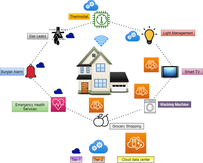
In this section, we discuss the problem formulation. Table I depicts the notation used in the rest of this paper. We consider a hierarchical fog-cloud architecture comprising of users at the lowest level. The user is denoted by . The users are connected to m tier-1 fog devices given by = {, ,……,,}. The tier-1 fog devices are followed by r tier-2 fog devices given by = {, ,……,,}. The tier-2 fog devices are further connected to p tier-n fog devices, such as, = {, ,……,,}. Note that, n can be any tier such as, tier-3, tier-4, and so on. At the topmost level, we have a cloud data center cdc C, where C is the set of all cloud data centers. The cloud data center cdc has the maximum execution execution capacity among all the tiers. The execution capacity of fog devices in is less than fog devices in , which is further less than . A similar hierarchical fog architecture has been outlined in [19]. The order of execution capacity is: . The units of execution capacity is MIPS, i.e., Millions of Instructions per Second. We have used MIPS as the unit of execution capacity, as the iFogSim simulator [20] measures the computational capability of execution devices in MIPS. iFogSim is a well known simulator that has been used to simulate fog, edge, and cloud networks[8]. A smart home example scenario is shown in Fig. 2. In the considered smart home scenario, the jobs which require a response within milliseconds, such as burglar alarm, gas leaks, etc. can be executed on the fog devices in . The jobs such as maintaining overall temperature of the home, switching lights on/off can be scheduled at fog devices in . Next, the weekly/monthly grocery shopping by tracking the consumption of food of the individuals can be executed at higher tiers with the nodes having higher computational capacity, where n = 3. Finally, the entertainment services such as recording some TV series to watch later can use the services of the cloud data center.
We consider a job set J, that can be executed on fog devices in , , …., , or the cdc. We considere a single cdc in our work. However, our work can be easily extended to multiple cloud data centers. The fog device at tier-1, tier-2, and tier-n is given by , , and respectively. Likewise, the job is given by . The delay between and is given by . Correspondingly, the delay between and is given by , and so on. Lastly, gives the delay between and cdc. We assume that the fog devices within each tier are homogeneous in nature, i.e., no “intra-level heterogeneity” has been considered. This implies that all fog devices in have identical execution capacities. This holds true for fog devices in , and fog devices in as well. However, all tiers, i.e., fog devices in , fog devices in , fog devices in , and cloud data center cdc are heterogeneous with respect to each other. In other words, we consider “inter-level heterogeneity” in our model. Intuitively, jobs with modest are executed at tier-1 fog devices by default, as they can be executed faster owing to the distance proximity from the user. Generally, the jobs with moderate are assigned to tier-2, or tier-n fog devices. Finally, the jobs with large cpu requirements are assigned to the cdc.
Job can be assigned to fog devices in , , , or the cdc, depending upon it’s execution cost and/or sufficient spare capacity in the fog device or the cloud. Let be the variable which denotes whether is assigned to a fog device or to the cloud data center:
| (1) |
In eq. (1) above, can be fog device present at tier ().
We need to make sure that each is assigned to a single fog device only. The following equation ensures this constraint:
| (2) |
The begin time bt of on a fd FD is denoted by . We assume that all jobs are independent of each other, so no precedence constraints are present among the jobs. Hence, theoretically a job may begin at time 0. The execution time of is represented by . The completion time of J on fd is designated by . The completion time of can be defined as:
| (3) |
The minimum completion time of a job can be calculated as:
| (4) |
In eq. (4) above, , and .
Next, we model the network usage of the system. This quantity is defined as the total data sent and received by various network devices: fog devices in , , , and the cloud data center cdc. Mathematically, can be defined as:
| (5) |
In eq. (5) above, is the data processed by , is the aggregate delay that occurs during the submission and execution of , and is the time for which the simulation was run.
Let us assume that the maximum amount of jobs that can be processed at fd is and that the job arrival rate at fd is . Note that, fd can be any fog device present at tier-1, tier-2, or tier-n. We follow an M/M/1 queuing system to process user jobs at each fog device [43]. The average completion time cost for at fd can be calculated as:
| (6) |
Likewise, we can model act of cdc as:
| (7) |
Let the average job execution capacity of fd be . We can derive the average energy consumption cost as follows:
The energy consumption of a fog device is directly proportional to the fog device’s computation power/execution capacity.
Similarly, can be defined as follows:
As each fog device has a limited resource capability, this means that the offloaded job’s must not exceed it’s .
Here is the remaining spare capacity of fd FD.
We assume that , ,…, be the cpu requirements of the jobs which are being offloaded to fog devices in . The probability that can run the with is given by . Hence, the probability that all tier-1 fog devices can schedule jobs with different cpu requirements can be defined as follows:
In case , this means tier-1 fog devices are unable to schedule the jobs based on their cpu requirement. In this case, the jobs are sent to the higher tiers for execution. Likewise, we can define the probability for all tier-2 fog devices, and tier-n fog devices. For the sake of brevity, we omit these equations.
The overall cost for all tier-1 fog devices can be written as:
The overall cost for all tier-2 fog devices can be written as:
A similar formulation can be carried out for all tier-n fog devices.
Likewise, we model the cost for the cloud:
The optimisation problem that we attempt to solve in this work is modelled as follows:
Given a set of jobs , a set of fog devices , , , and a cloud data center cdc, with inter-level heterogeneity, schedule the jobs onto fog tiers/cdc by using FiFSA & EFSA such that the overall cost is minimised. Formally,
| subject to | |||||
IV Proposed Algorithm
We now describe the working of the two proposed algorithms for scheduling jobs on multi-tiered fog-cloud architectures : FiFSA and EFSA.
The steps involved in the working of FiFSA are described below:
-
1.
In the first step, all the jobs are arranged in increasing order of in Q.
-
2.
The of fog devices in is compared with . If the current fog device has spare capacity to run , then the job is scheduled on . The value of flag is set as 1.
-
3.
Otherwise, the of fog devices in is compared with . If the fog device can run the job, then is scheduled on .
-
4.
Otherwise, we check the capacity of tier-3 fog devices, and so on till we obtain an appropriate fog tier to run .
-
5.
Finally, if none of the , , or are capable of scheduling , the job is then scheduled on the cloud data center cdc.
-
6.
Calculate .
Note that while selecting the fog device to schedule a job, we evaluate all fog devices present at that tier sequentially. Once we identify a fog device which has sufficient spare capacity, we assign the job to the fog device and set the variable flag, and move on the next job. If no fog device at tier-1 is able to schedule the job, we proceed to the tier-2 fog layer, and so on.
We now discuss the functioning of the proposed scheduling algorithm EFSA. Here, we create different queues for each fog-tier according to of the jobs. The steps involved in the working of EFSA are described below:
-
1.
The of fog devices in is compared with . If the job’s cpu requirement is within the execution capacity of fog devices in , then the job is populated in . However, if the cpu requirement of job is more than the capacity of that fog-tier, then it is moved to the next tier, else it is placed in the queue of the same tier.
-
2.
Otherwise, is compared with the capacity of fog node in . If the job can be run with the execution capacity of tier-2 fog devices, then job is added to .
-
3.
Likewise, we populate the jobs in by measuring the with the execution capacity of fog devices present at the tier-n .
-
4.
The remaining jobs are scheduled on the cloud data center .
We use the min-min scheduler to execute the jobs present at fog devices in , fog devices in , and on fog devices in . The rationale behind choosing the min-min scheduler is that it finds the job with smallest completion time and assigns it to the fastest fog device. This fog device is selected by using the procedure MinMinNode(, , , ).
The Min-Min procedure works as follows:
-
1.
For each , , and present at each tier , , and respectively, we use the Min-Min scheduler for the job execution at each tier separately [23].
-
2.
The Min-Min heuristic works in N iterations, where N is the number of jobs which need to be scheduled.
-
3.
This heuristic consists of two steps, as outlined below:
-
•
In the first step, the heuristic finds the minimum completion time MCT of each unassigned job over the set of fog devices. It finds the best fog device i.e. the fog device which can finish the job in the earliest time. The algorithm takes into account the current load as well as completion time while finding the best fog device for job scheduling.
-
•
In the second step, the heuristic chooses the unassigned job which has the minimum MCT among all jobs. This job will be assigned to the best fog device found in the first step.
-
•
The scheduled job is removed from the queue, and is not considered in the rest of the iterations.
-
•
-
4.
The above process is repeated until all jobs present in different queues have been scheduled.
-
5.
Finally, is calculated.
In FiFSA, we first sort the jobs in an increasing order of cpu requirement. We note that the fog devices at low tiers have modest execution capacities. Hence, it may not be advisable to schedule the jobs with high cpu requirements on lower tiers. Once we identify a fog device having sufficient spare capacity, we schedule the job on it. Otherwise, we keep checking fog devices on higher tiers. For the second algorithm, EFSA use the MinMin scheduler. MinMin is a fast and simple algorithm that considers smaller jobs first, and assigns them to fast processors, which in turn minimises the completion time. This aligns well with our hierarchical architecture, as the fog devices at lower tiers have lower execution capacity as compared to fog devices present at higher tiers.
IV-A Complexity Analysis of FiFSA and EFSA
We assume that there are total of jobs that need to be scheduled, such that . Here, are the number of jobs that will be scheduled on fog devices and are the number of jobs that will be scheduled on the cloud data centers cdcs. Let be the total number of fog devices and cdcs, such that . Here, is the number of fog devices and is the number of cdcs. In FiFSA, the jobs are populated in Q, for a complexity of . In the next step, the jobs are sorted in increasing order of cpu requirement. The complexity of this stage is . The cpu requirement is checked for each job in the next stage and jobs are assigned to fog devices or cdcs. The complexity of this stage is . Finally, we calculate the of all jobs. The complexity of this step becomes . By adding all these terms, + + + , the overall complexity for FiFSA becomes .
In EFSA, the cpu requirement is checked for each job in the first step. If the requirement is met, then the job is added to the corresponding queue. The complexity of this stage is . The jobs are either assigned to the cdc or to the fog devices, according to the queues. As we are working with a class of assignment problems which are polynomially solvable, this makes the complexity of cloud scheduler [14]. We use the min-min scheduler in EFSA. The complexity of the min-min scheduler is [6]. Finally, we calculate for the jobs, for a complexity of and on fog devices and cdc respectively. On adding all these terms, we get + + + + . This gives us the complexity expression + .
V Simulation Results and Analysis
We now discuss the results of the simulations that have been carried out to analyse the performance of the proposed algorithms : FiFSA and EFSA. We consider various simulation scenarios and evaluate the performance for each scenario. The considered sample scenarios align with our fog architecture introduced in Fig 1. The jobs may execute on : tier-1 fog devices, tier-2 fog devices, tier-3 fog devices, tier-4 fog devices, and the cloud data center cdc. We have considered several tiers of fog devices to measure the performance of the algorithms on different architectures. The proposed model can be extended to a larger number of tiers, as per the requirements of the application. In FiFSA, the jobs execute on the respective tiers as per their . If of a tier-1 fog device is sufficient to meet the requirements of , then will execute on tier-1, otherwise it will be dispatched to tier-2 for execution. Again, of a tier-2 fog device is checked, if it is sufficient, then job can execute on tier-2. If it’s not sufficient, then further tiers are checked for job execution. If the job is still unscheduled on all examined fog tiers, it is executed on the cdc. We compare the results of four algorithms: FiFSA, EFSA, LTF, and cdc-only. In cdc-only, the jobs execute only on the cloud data center, without considering the fog devices. The EFSA algorithm schedules the job on the fog device by finding the MinMinNode onto various fog tiers. We use MinMinNode and elected fog device interchangeably in the paper. The LTF (Longest Time First) algorithm has been proposed In [47]. LTF assigns the job with the longest execution time to the fog node which executes it in the minimum time i.e fastest node.
V-A Workload
We now discuss the workload that has been used as an input for our simulation scenarios. In order to make the simulations more meaningful, a real workload trace named the “Alibaba Cluster Trace” Program [1] has been used. The is the file that consists of cluster information of about 1300 machines. The production cluster consists of both online and batch jobs. The system has been evaluated for a period of 24-hours. This workload can be used to assign the jobs to various machines and cpus, while improving the resource utilisation. It can also be used to explore the trade off in the resource allocation between online services and batch jobs, with a balanced goal of providing better throughput to batch jobs as well as maintaining the satisfactory service quality of the online services. The workload consists of various fields: , , , , and . The fog environment considered for simulation has fog devices in , fog devices in , fog devices in , fog devices in , and a proxy server that is connected to a cloud data center cdc. The fog devices in are connected to various sensors and actuators. We have considered diverse number of fog tiers along with diverse number of fog devices within each tier as per sample architectures. The detailed information about these architectures is provided in Section 5.2. We consider the fog devices within a particular tier to be homogeneous. This means that within a particular tier, the computation capacities of all fog devices are identical. As one moves up in the tiers, the capacity of fog devices increases. On the flip side, moving to higher tiers leads to an increase in the delay between the user and fog devices.
V-B Hierarchical Fog-Cloud architecture
We consider four types of hierarchical fog cloud architectures in our work. The description of these architectures is as follows:
-
•
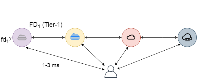
Flat hierarchy: This architecture consists of five fog devices in , followed by the cloud data center cdc, as shown in Fig. 4. The from to varies from 1 millisecond to 3 milliseconds, and from to is fixed at 140 milliseconds. The MIPS capacity of is denoted by . Likewise, the MIPS capacity of the cdc is denoted by . The and is fixed at 2000 MIPS and 57980 MIPS respectively.
-
•
2-tier hierarchy: This architecture consists of five fog devices in , followed by five fog devices in , and the cloud data center cdc at the top of the hierarchy, as shown in Fig. 1. The from to fog devices in varies from 1 millisecond to 3 milliseconds, from to fog devices in varies from 4.1 millisecond to 9 milliseconds and from to is fixed at 140 milliseconds. The and is fixed at 2000 MIPS and 3500 MIPS respectively. Likewise, the is fixed at 57980 MIPS respectively.
-
•
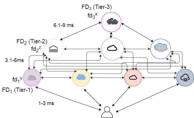
3-tier hierarchy: In this architecture, we have considered an extension of the 2-tier hierarchy by adding an extra layer of fog devices between fog devices in and cloud data center cdc, as described in Fig. 4. We have considered a single fog device at tier-3 of the architecture. The is taken as 6500 MIPS. The between to fog device in varies from 10.2 milliseconds to 18 milliseconds.
-
•
4-tier hierarchy: This architecture is an extension of the 3-tier hierarchy, as shown in Fig. 5. We have considered a single fog device in between and cdc. The is taken as 8500 MIPS. The between to fog device in varies from 19.3 milliseconds to 30 milliseconds. The from to is fixed at 140 milliseconds.
Note that these are representative values. Based on the user/application specifications, these values can be modified without effecting the functioning of the algorithms. In addition, we have created a representational network for the sake of the simulations. The simulator allows users to vary this as well, based on the requirement.
V-C Simulation setup and parameters
The simulations has been run on an HP workstation with 7.7 GB RAM, Intel core i7-7700 CPU @ 3.60GHz processor, 64-bit Ubuntu OS 18.04 LTS. The proposed algorithms have been implemented on the iFogSim simulator [20]. Many fog applications have been modeled by researchers using iFogSim [15, 44]. iFogSim provides a range of functionalities, which makes it a suitable option for simulating various characteristics of fog devices, jobs, and the cdc. The simulator consists of a resource management module which manages the resource allocation policies in the fog and cloud environment. In order to implement the proposed algorithms, we created two classes in iFogSim: a random class and an elected class. The random class implements FiFSA and the elected class implements EFSA. The and hierarchy of fog devices has been created in these two classes separately. For each hierarchy, we have formed a separate class, such as, EFSA 4-tier class, EFSA 3-tier class, EFSA 2-tier class, EFSA flat-tier class, FiFSA 4-tier class, FiFSA 3-tier class, FiFSA 2-tier class, and FiFSA flat-tier class. The parameters such as d, cp(FD), cp(cdc), up-link bandwidth, down-link bandwidth and module mapping are described in the classes.
The parameters that have been used in the simulation scenarios are as follows:
-
•
Job load (JL): Each job has some MIPS requirement associated with it. The initial MIPS requirement has been taken from the workload trace. Next, we calculated the average MIPS value for all jobs. After the first assignment, the average MIPS value of the jobs is multiplied from 1.5 to 4. Specifically, the MIPS value has been multiplied by 0.5 in each iteration, to obtain various data points.
-
•
Delay (d): This parameter defines the range of communication delay between the jobs, , , , , and cdc. The parameter d from to varies from 1 millisecond to 3 milliseconds, d between to varies from 3.1 milliseconds to 6 milliseconds, d between to varies from 6.1 milliseconds to 9 milliseconds, and d between to varies from 9.1 milliseconds to 12 milliseconds. The parameter d between to cdc is 140 milliseconds. The initial delay parameters are taken in the first iteration. After that, the delay is increased by 5 milliseconds at each tier.
-
•
Network Usage (NU): This quantity is defined as the total data sent and received by various network devices present at , , , , and the cdc.
-
•
Total completion time (tct): This parameter is defined as the time at which all the submitted jobs complete their execution.
V-D Effect of fog on system performance
In this section, we discuss the performance of the proposed scheduling algorithms on multi-tiered fog-cloud architectures. In order to evaluate the performance, we - (i) carry out extensive simulations and (ii) implement a prototype. We discuss the results for flat-tiered, 2-tiered, 3-tiered, and 4-tiered fog architecture, as shown in figures 3, 1, 4 and 5 respectively. This means that the jobs can be processed at: fog devices in , , , , or at the .
V-D1 Effect of job load on total completion time
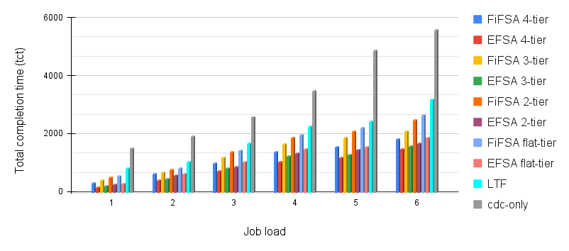
The motivation here is to illustrate the advantage of employing fog devices to enhance the capability of the cdc. We compare the proposed algorithms with cdc-only and LTF. In LTF, two types of fog devices have been considered : slow nodes and fast nodes. We consider 5 nodes as slow and 1 node as fast. The average speed of the nodes is calculated in MIPS. The nodes which have a speed less than the average node speed are considered as slow, and the nodes which have a greater speed than the average node speed are considered as fast nodes. We first calculate the average MIPS of the original trace. After this, the average MIPS value is multiplied from 1.5 to 4, with an interval of 0.5 at each iteration in order to get a range of job loads. The Job Load (JL) has been increased, and its effect on the observed tct has been recorded for all algorithms. The results are shown in Fig. 6. It has been observed that tct increases with an increase in the JL. In general, increasing the job load adds more computation on the system, which results in increasing the overall tct. We observe that the highest tct is demonstrated by the cdc-only algorithm. The reason for this is that all jobs are allocated to the cloud data center in cdc-only, which leads to higher tct, owing to the greater physical distance from to the cdc. The FiFSA algorithm offers higher tct as compared to the EFSA algorithm. This can be explained as follows. FiFSA assigns the jobs to fog devices on the basis of the SJF (Shortest Job First) technique. It maps the shortest job to the first available fog device with sufficient execution capacity. The fog device on which the job is assigned may or may not be best candidate for execution. It may so happen that the job is assigned to a fog device that is farther from the user, therefore there could be an increase in the tct. On the other hand, in the EFSA algorithm, we calculate the finish times of the jobs on all available fog devices. Next, we assign the job on the elected fog device which ensures the minimum finish time. This results in lower tct for EFSA. The LTF algorithm assigns jobs with the largest execution time to the fastest node at each level. This makes the waiting time of the short jobs larger, and increases the overall completion time of LTF. Hence, we observe that the offered by the LTF algorithm is more than that offered by both FiFSA and EFSA, but less than what is offered by cdc-only.
Here, we discuss the effect of job load on tct for flat-tiered, 2-tiered, 3-tiered and 4-tiered fog hierarchies. We observe that the best performance is offered by the 4-tier hierarchy for both proposed algorithms. The reason for this is that the overall computation capacity of the 4-tier hierarchy is higher than the other hierarchies. This decreases the overall tct of the proposed algorithms. Though the fog devices present at are at greater distance from , but sending jobs to tier-4 incurs much less delay as compared to sending jobs to the cdc. In addition, the fog devices present at tier-4 have higher computation power than the devices present at lower tiers. The next best performance is offered by 3-tier hierarchy. By removing tier-4 from the architecture, more jobs are sent to the cloud, which increases the tct. The decrease in the computation power results in a higher tct. The 2-tier hierarchy performs in between the 3-tier hierarchy and the flat-tier hierarchy. The worst performance is offered by the flat hierarchy owing to sending a larger number jobs to the cdc, after reaching the computation threshold of tier-1 fog devices. Note that, there isn’t much difference in the tct of different hierarchies within each algorithm in the starting phase i.e. when job load is less. This happens because most of the jobs are able to finish execution on the lower tiers initially. However, with the increase in the job load, more jobs are offloaded to the higher fog tiers due to the modest capacity of lower fog devices. Our proposed algorithm optimises the offloading of the jobs by using the EFSA algorithm. We observe that EFSA offers a better performance than FiFSA for all the hierarchies. This happens as EFSA doesn’t assign jobs randomly to the fog devices or fog tiers on the basis of SJF. It calculates the MinMinNode for the job execution. With more number of tiers in FiFSA, there are more chances of sending the jobs to the farther fog device once the threshold of the current tier is reached. The tct provided by all scheduling hierarchies is as follows: 4-tier 3-tier 2-tier flat-tier 4-tier 3-tier 2-tier flat-tier cdc-only.
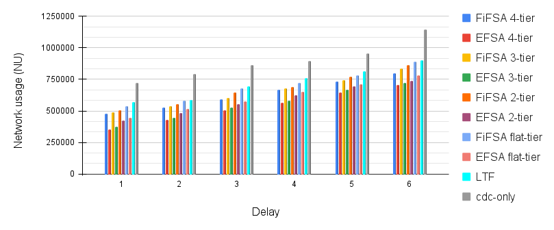
V-D2 Effect of job load on network usage
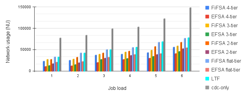
In this simulation, we observe the effect of job load (JL) on overall network usage (). Basically, network usage is the data transferred among various fog devices present at , , , and the cdc. This is calculated by multiplying the transferred data and delay between source and destination and dividing the result by the simulation time. Here, simulation time is the time for which the simulation was run. We observe that when we increase the job load, the data communication of the respective jobs increases as well. The results are shown in Fig. 7. It is observed that the network usage is maximum in cdc-only. This happens as network usage is directly proportional to the delay incurred, and the data has to travel all the way from the user to the cdc. The network usage of the FiFSA algorithm is more than that of the EFSA algorithm, but less than that of cdc-only. It is less than cdc-only as FiFSA algorithm incorporates fog devices as well, due to which there is lesser propagation delay overall. However, the proposed EFSA algorithm doesn’t allocate the jobs to fog devices randomly. It finds the elected fog node for the job which finishes the execution in minimum time, for all fog-tiers. Hence, the network usage is minimum for the EFSA algorithm. The LTF algorithm reports marginally higher network usage than that reported by the FiFSA algorithm, as both algorithms use fog devices for job execution. However, the former uses the longest job first technique and the latter uses the shortest job first technique.
Next, we estimate the effect of job load on network usage over flat-tiered, 2-tiered, 3-tiered, and 4-tiered fog hierarchies. The maximum network usage is observed for the flat hierarchy, for both FiFSA and EFSA algorithms. The reason for this is that with an increase in job load, it becomes hard for a single fog tier to ensure timely job execution. Hence, more jobs are offloaded to the cdc for computation, and this increases the delay for these jobs. This leads to an increase in the network usage of the system. The best performance is offered by the 4-tier hierarchy, as it can accommodate more jobs within the fog tiers, which results in reduced overall transmission delay. The next best performance is offered by the 3-tier hierarchy. The removal of the fourth fog tier increases the network usage due to the transmission of more jobs from to the cdc. With the decrease in the overall computation power offered by the 3-tier and 2-tier architectures, the network usage increases in the same order. With large job loads, there is larger reduction in network usage in tiered hierarchy as compared to the flat hierarchy. The overall network usage of the hierarchies is as follows: 4-tier 3-tier 2-tier flat 4-tier 3-tier 2-tier flat LTF cdc-only.
V-D3 Effect of delay on total completion time
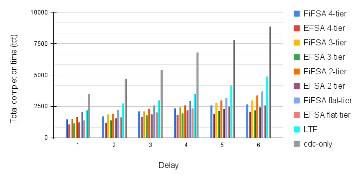
Next, we discuss the effect of propagation delay (, from a job to fog devices or to the cdc) on the . The job load and the fog device count has been kept constant in order to study the effect of delay on the job’s tct. The delay has been increased by 5 milliseconds at each stage. Intuitively, the tct increases with increase in the delay, as the communication becomes a bottleneck. The results of this simulation are shown in Fig. 8. We observe that by increasing d, the finish times of jobs gets advanced in all algorithms. As mentioned in the previous section, the EFSA algorithm outperforms FiFSA and LTF due to the selection of elected fog node at each tier, which results in efficient utilisation of fog devices. The cdc-only algorithm offers the highest tct as fog devices are not employed for job execution. Additionally, the induced delay from to cdc results in increasing the communication time, which in turn increases the tct.
Next, we discuss the effect of delay on the job’s tct for flat-tiered, 2-tiered, 3-tiered and 4-tiered fog hierarchies. Similar to previous sections, the 4-tier hierarchy offers the best results, and the flat hierarchy performs the worst, due to the trade-off between computation power and communication delay. This means that EFSA 4-tier performs the best among rest of the scheduling strategies i.e. EFSA 3-tier, EFSA 2-tier, and EFSA flat-tier. Likewise, FiFSA 4-tier performs the best among rest of the scheduling strategies i.e. FiFSA 3-tier, FiFSA 2-tier, and FiFSA flat-tier. However, the increased d impacts all four hierarchies, for both FiFSA and EFSA. This happens as the delay is directly proportional to the job’s tct. So, the overall tct of the jobs gets extended for all four hierarchies, which is visible in the results. The overall tct is as follows: 4-tier 3-tier 2-tier flat-tier 4-tier 3-tier 2-tier flat-tier .
V-D4 Effect of delay on network usage
In this simulation, we study the effect of delay on network usage. As network usage is directly proportional to the delay, this means that network usage will increase on increasing the delay. In this simulation, the delay is increased by 5 milliseconds for each point present on the x-axis. We have kept the job load and fog device count constant to measure the effect of delay on network usage. The results are shown in Fig. 9. The least network usage is offered by the EFSA algorithm. EFSA outperforms others as a smaller path needs to be travelled for executing the jobs on their elected fog devices. FiFSA and LTF perform almost the same in the simulation, as they both use fog devices for executing jobs, but the former chooses fog device randomly from the tiers after applying SJF, and the latter assigns the longest job first to run on the fog device that offers minimum execution time. Lastly, in cdc-only, the jobs need to travel all way from the user to the cloud, which results in more network usage.
Next, we observe the effect of delay on network usage over various hierarchies: EFSA 4-tier, EFSA 3-tier, EFSA 2-tier, EFSA flat-tier, FiFSA 4-tier, FiFSA 3-tier, FiFSA 2-tier, and FiFSA flat-tier. Intuitively, the network usage increases with the increase of delay between fog devices FD and cdc-only. The least network usage is offered by EFSA 4-tier hierarchy. This happens as the algorithm employs four tiers of fog devices, which increases the overall computation power of the system. Along with this, a lesser number of jobs need to travel to the cloud data center, as the jobs can be executed onto the tiers of the architecture which incurs less delay. The EFSA algorithm also uses MinMinNode to run the jobs onto several tiers. This decreases the overall network usage of EFSA 4-tier. The next best performance is offered by EFSA 3-tier, EFSA 2-tier, and EFSA flat-tier in the same order. This occurs because as we decrease the number of tiers of fog devices, more jobs are sent to the cloud data center for the execution. This increases the network usage of the system. For FiFSA algorithm, FiFSA 4-tier outperforms all other tiers: FiFSA 3-tier, FiFSA 2-tier, and FiFSA flat-tier. The EFSA outperforms FiFSA for all tiers. The reason for this is that the FiFSA algorithm can schedule the jobs to the farthest fog device once the capacity of the lower tier fog devices has been exhausted.
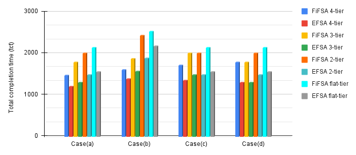
V-D5 Effect of change in the number of fog devices on total completion time
This section explores the effect of fog processor/device count on the system’s tct. Specifically, we observe how the algorithms adapt to the change in the number of fog devices. Initially, we consider ten fog devices (five at and five at ). The and has been fixed at 2000 MIPS and 3500 MIPS respectively. We consider a single fog device at and at . The and has been fixed at 6500 MIPS and 8500 MIPS respectively. The job load and delay have been kept constant at each stage to focus on the effect of processor count. The results of this simulation are shown in Fig. 10. We consider four cases. In case(a), all the fog devices are considered at all tiers. In case(b), a single fog device is removed, from both and . In case(c), the lone fog device at is removed, and in case(d), the fog device at is removed. For case(a), we can see a similar performance trend of all the hierarchies as discussed in the previous sections. In case(b), as there is a decrease in the fog device count at and at , we observe an increase in the tct for all the hierarchies. However, this increase is more prominent in FiFSA 2-tier, FiFSA flat-tier, EFSA 2-tier, and EFSA flat-tier. This occurs due to a decrease in the computation power that leads to advanced tct. We observe a marginal increase in the tct of FiFSA 4-tier, FiFSA 3-tier, EFSA 4-tier, and EFSA 3-tier. The reason for this is that fog devices are present at higher tiers to manage load execution if some fog device become non-functional/ unavailable at lower tiers. In case(c), there is no effect on the tct of FiFSA 2-tier, FiFSA flat-tier, EFSA 2-tier, and FiFSA flat-tier. These fog device hierarchies do not employ the third tier of fog devices in their architecture. So, their behavior is quite similar to case(a). As the third tier becomes non-functional in FiFSA 3-tier and EFSA 3-tier, both of the algorithms start behaving like FiFSA 2-tier and EFSA 2-tier. We observe an increase in the tct for FiFSA 4-tier and EFSA 4-tier. With a non-functional third tier, more jobs are sent to tier-4 for execution. However, tier-4 is present at a larger distance as compared to tier-3. For case(d), only a 4-tier hierarchy gets affected, as none of the 3-tier, 2-tier, flat-tier hierarchies employ the fourth fog device tier. The algorithms FiFSA 4-tier and EFSA 4-tier start behaving like their 3-tier equivalents, FiFSA 3-tier and EFSA 3-tier respectively.
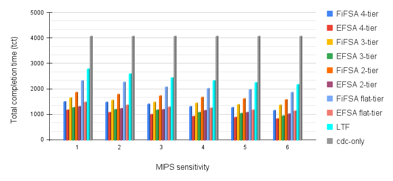
V-D6 Effect of MIPS sensitivity on total completion time
In this simulation, we investigate the effect of changing fog device MIPS sensitivity on the system performance. The execution capacity of the cdc is the same as in earlier simulations. The has been varied from 2000 to 3500 MIPS and has been varied from 3500 to 5000 MIPS. Likewise, has been varied from 6500 to 8000 MIPS and has been varied from 8500 to 10000 MIPS. Essentially, we increase the execution capacity by 300 MIPS at each stage. In the first data point on the x-axis, , , , and has been kept at 2000 MIPS, 3500 MIPS, 6500 MIPS, and 8500 MIPS respectively. For the second x-axis data point, these values have been increased by 300 MIPS, and so on. We have kept the job load constant in this simulation. The results of this simulation are shown in Fig. 11. As expected, the response time for cdc-only is constant for each iteration. On the other hand, the response time for FiFSA, EFSA and LTF decreases with the increase in MIPS capacity. The reason behind this behaviour is that with an increase in the MIPS capacity of fog devices, we are increasing the computation power at each tier. With the increase in the computation power, more jobs can be accommodated by the fog devices, which leads to a decrease in the tct of jobs.
Next, we analyse the effect of MIPS sensitivity on several fog hierarchies. It is evident from the results that with the increase of MIPS values, there is a decrease in the tcts. With an increase in computation power, more jobs are able to finish their execution on the fog devices. This decreases the overall job tct. The results for this simulation are as follows: 4-tier 3-tier 2-tier flat-tier 4-tier 3-tier 2-tier flat-tier .
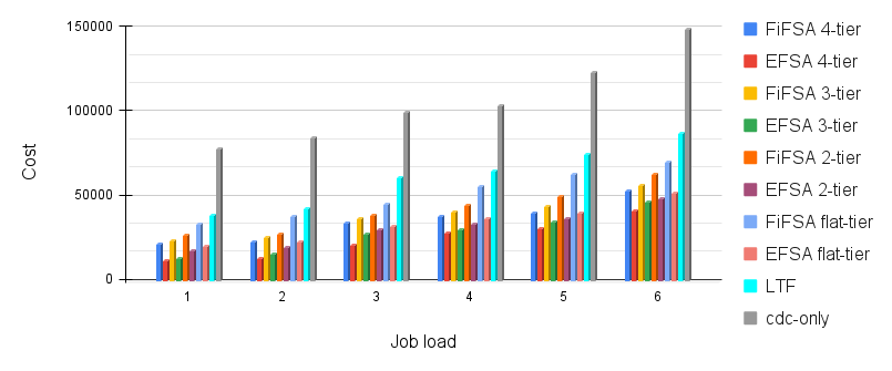
V-D7 Effect of job load on cost
In the next simulation, we observe the effect of job load on the system cost . We have taken and as 2000 MIPS and 3500 MIPS respectively. Further, and has been picked as 6500 MIPS and 8500 MIPS respectively. As we can see in Fig. 12, the maximum cost is demonstrated by cdc-only. The cost is the summation of average completion time and average energy consumption. Both completion time and energy consumption are high in cdc-only, which leads to a higher cost. As stated earlier, the average completion time of FiFSA is higher than that of EFSA. FiFSA does not take into account the suitable fog device for executing the job at the respective tiers. This results in higher average completion times, as well as higher average energy consumption, thus making the cost of FiFSA more than that of EFSA. Additionally, LTF offers a higher cost than FiFSA and EFSA, as LTF takes more time in finishing the jobs. This increases the average completion and average energy consumption of LTF. Besides, there is an increase in the cost for all four algorithms FiFSA, EFSA, LTF, and cdc-only with the addition of the job load. This happens due to the following - by adding job load on the system, it becomes difficult for fog devices to run the jobs in a timely manner, which in turn increases the overall cost.
With the increase of job load, we observe a gradual increase in the cost for all hierarchies present in FiFSA and EFSA. The best performance is offered by EFSA 4-tier and worst performance is given by FiFSA flat-tier. This occurs because EFSA 4-tier employs four tiers of fog devices along with the usage of a superior heuristic. On the other hand, FiFSA flat-tier has only a single tier of fog devices, and it assigns the jobs on the basis of SJF without actually finding the elected fog device. Due to this, cost of FiFSA flat-tier is more than EFSA 4-tier. We observe a similar trend in tier-wise performance of both the algorithms due to the reasons mentioned in the previous sections.
V-E Fog Cloud Testbed
In order to validate our simulation results, we designed and created a working prototype to evaluate the performance of the two proposed algorithms : FiFSA and EFSA on a hierarchical fog-cloud architecture. We formed two tiers of fog devices followed by the cloud data center cdc. We employed two Raspberry Pi 4 Model B devices at of the architecture. A desktop with Ubuntu 18.04 operating system has been used as an . Finally, we used a cloud VM instance with 1 vCPU, 1 GiB memory as the cdc. The cdc was present in the Asia Pacific (Mumbai) ap-south-1 region. Both raspberry pis are equipped with Broadcom BCM2711, Quad core Cortex-A72 (ARM v8) 64-bit SoC 1.5GHz running Raspbian OS. is an Intel i7-7700 CPU, 3.60GHz 8, 64-bit OS with 7.7GiB RAM. The fog devices were connected through Wifi, which was able to provide service up to a distance of 60 meters. We set the first raspberry pi and second raspberry pi at distances of 2 meters and 10 meters respectively from the WiFi hotspot. The fog device desktop PC was located 20 meters from the WiFi hotspot. We used an IPv4 Internet connection to connect the user to the cloud.
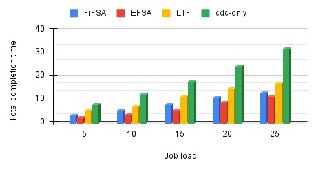
V-E1 Total completion time
In the first experiment, we observe the impact of job load on tct of FiFSA, EFSA, LTF, and cdc-only. Initially, we considered five jobs, and scheduled them using all four scheduling strategies mentioned above. Next, we started increasing the number of jobs (up to 25) in the job set and captured the tct. The results of this experiment are shown in Fig. 13. In case of cdc-only, we observe that the tct increases significantly when we increase the number of jobs in the job set. This happens due to the increase in the overall propagation delay between and cdc. On the other hand, the proposed algorithms FiFSA and EFSA offer lower tct, owing to the incorporation of fog devices for job execution. The tct offered by LTF is lower than that offered by cdc-only, but worse than the tct offered by FiFSA and EFSA. This is because LTF prefers to schedule the long jobs first. This increases the waiting time of the short jobs, leading to higher tcts.
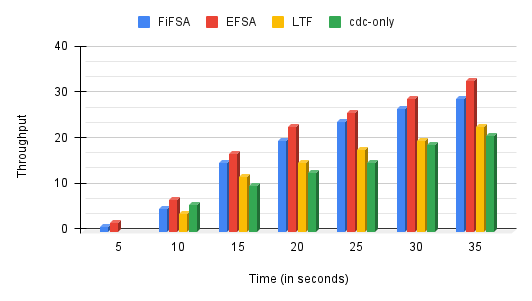
V-E2 Throughput
In the next experiment, we observe the system throughput for all four scheduling strategies. In order to determine the system throughput, we track the number of jobs that finished their execution in the specified amount of time. The results are shown in Fig. 14. As expected, the throughput increases with time for all the four algorithms: FiFSA, EFSA, LTF, and cdc-only. This happens because with the increase in the specified time, a larger number of the jobs are able to finish their execution. However, our proposed scheduling algorithms FiFSA and EFSA offer higher throughput than other compared algorithms due to the employment of fog devices and usage of superior heuristics. The highest throughput is offered by EFSA, as it assigns the shortest job to the fog device that can finish the job in the minimum amount of time.
VI Conclusion
There is a significant propagation delay involved in executing the jobs on cloud data centers. This delay can be reduced significantly by incorporating fog devices. Application requirements, such as smart transportation, often necessitate the consideration of a hierarchical fog-cloud model, with many layers of fog nodes. In this paper, we propose two algorithms that schedule jobs on such multi-tiered fog networks: FiFSA and EFSA. We take job characteristics such as cpu requirement into account, while scheduling them on various fog tiers (up to 4 fog tiers) and the cloud data center. The idea is to allocate the jobs on appropriate fog devices or the cloud data center, while minimising the overall cost. We compared the performance of both algorithms with cdc-only and the LTF algorithm, for a number of scenarios. The simulation results on a real-life workload and a testbed show that EFSA offers the best performance in terms of cost, completion time and network usage. In the future work, we aim to integrate multiple cloud data centers. Additionally, we plan to work on both ”inter-level heterogeneity” and ”intra-level heterogeneity” in our model.
References
- [1] Alibaba inc. cluster data collected from production clusters in alibaba for cluster management research. https://github.com/alibaba/clusterdata, 2017.
- [2] Raafat O Aburukba, Mazin AliKarrar, Taha Landolsi, and Khaled El-Fakih. Scheduling internet of things requests to minimize latency in hybrid fog-cloud computing. Future Generation Computer Systems, 111:539–551, 2020.
- [3] Ian F Akyildiz, Max Pierobon, Sasi Balasubramaniam, and Y Koucheryavy. The internet of bio-nano things. IEEE Communications Magazine, 53(3):32–40, 2015.
- [4] Abdulaziz Aljabre. Cloud computing for increased business value. International Journal of Business and social science, 3(1), 2012.
- [5] Bruno Andò, Salvatore Baglio, Antonio Pistorio, Giuseppe Marco Tina, and Cristina Ventura. Sentinella: Smart monitoring of photovoltaic systems at panel level. IEEE Transactions on Instrumentation and Measurement, 64(8):2188–2199, 2015.
- [6] Soheil Anousha and Mahmoud Ahmadi. An improved min-min task scheduling algorithm in grid computing. pages 103–113, 2013.
- [7] Michael Armbrust, Armando Fox, Rean Griffith, Anthony D Joseph, Randy Katz, Andy Konwinski, Gunho Lee, David Patterson, Ariel Rabkin, Ion Stoica, et al. A view of cloud computing. Communications of the ACM, 53(4):50–58, 2010.
- [8] Luiz F Bittencourt, Javier Diaz-Montes, Rajkumar Buyya, Omer F Rana, and Manish Parashar. Mobility-aware application scheduling in fog computing. IEEE Cloud Computing, 4(2):26–35, 2017.
- [9] Flavio Bonomi, Rodolfo Milito, Preethi Natarajan, and Jiang Zhu. Fog computing: A platform for internet of things and analytics. Big data and internet of things: A roadmap for smart environments, pages 169–186, 2014.
- [10] Rodrigo N Calheiros, Amir Vahid Dastjerdi, Harshit Gupta, Soumya K Ghosh, and Rajkumar Buyya. Fog computing: Principles, architectures, and applications. Internet of things, pages 61–75, 2016.
- [11] Luca Catarinucci, Danilo De Donno, Luca Mainetti, Luca Palano, Luigi Patrono, Maria Laura Stefanizzi, and Luciano Tarricone. An iot-aware architecture for smart healthcare systems. IEEE internet of things journal, 2(6):515–526, 2015.
- [12] Djabir Abdeldjalil Chekired, Lyes Khoukhi, and Hussein T Mouftah. Industrial iot data scheduling based on hierarchical fog computing: A key for enabling smart factory. IEEE Transactions on Industrial Informatics, 14(10):4590–4602, 2018.
- [13] Cisco. Fog computing the internet of things: Extend the cloud to where the things are. White Paper, 2015.
- [14] H Cui, J Zhang, C Cui, and Q Chen. Solving large-scale assignment problems by kuhn-munkres algorithm. pages 822–827, 2016.
- [15] Bilal Khalid Dar, Munam Ali Shah, Huniya Shahid, and Adnan Naseem. Fog computing based automated accident detection and emergency response system using android smartphone. In 2018 14th International Conference on Emerging Technologies (ICET), pages 1–6. IEEE, 2018.
- [16] Haluk Demirkan. A smart healthcare systems framework. It Professional, 15(5):38–45, 2013.
- [17] Elie El Haber, Tri Minh Nguyen, and Chadi Assi. Joint optimization of computational cost and devices energy for task offloading in multi-tier edge-clouds. IEEE Transactions on Communications, 67(5):3407–3421, 2019.
- [18] Qiang Fan and Nirwan Ansari. Workload allocation in hierarchical cloudlet networks. IEEE Communications Letters, 22(4):820–823, 2018.
- [19] OpenFog Consortium Architecture Working Group et al. Openfog reference architecture for fog computing. 2017. URL: https://www. openfogconsortium. org/wp-content/uploads/OpenFog_Reference_Architecture_2 _09_17-FINAL.pdf.
- [20] Harshit Gupta, Amir Vahid Dastjerdi, Soumya K Ghosh, and Rajkumar Buyya. ifogsim: A toolkit for modeling and simulation of resource management techniques in the internet of things, edge and fog computing environments. Software: Practice and Experience, 47(9):1275–1296, 2017.
- [21] Debiao He and Sherali Zeadally. An analysis of rfid authentication schemes for internet of things in healthcare environment using elliptic curve cryptography. Comput Method Appl M, 2(1):72–83, 2014.
- [22] Bidoura Ahmad Hridita, Mohammad Irfan, and Md Shariful Islam. Mobility aware task allocation for mobile cloud computing. International Journal of Computer Applications, 137(9):35–41, 2016.
- [23] O.H. Ibarra and C.E. Kim. Heuristic algorithms for scheduling independent tasks on nonidentical processors. Journal of the ACM (JACM), 24(2):280–289, 1977.
- [24] Jiong Jin, Jayavardhana Gubbi, Slaven Marusic, and Marimuthu Palaniswami. An information framework for creating a smart city through internet of things. IEEE Internet of Things journal, 1(2):112–121, 2014.
- [25] Joao Lima. https://www.cbronline.com/internet-of-things/10-of-the-biggest-iot-data-generators-4586937/. 2015.
- [26] Tingting Liu, Jun Li, BaekGyu Kim, Chung-Wei Lin, Shinichi Shiraishi, Jiang Xie, and Zhu Han. Distributed file allocation using matching game in mobile fog-caching service network. In IEEE INFOCOM 2018-IEEE Conference on Computer Communications Workshops (INFOCOM WKSHPS), pages 499–504. IEEE, 2018.
- [27] Yiming Liu, F Richard Yu, Xi Li, Hong Ji, and Victor CM Leung. Hybrid computation offloading in fog and cloud networks with non-orthogonal multiple access. In IEEE INFOCOM 2018-IEEE Conference on Computer Communications Workshops (INFOCOM WKSHPS), pages 154–159. IEEE, 2018.
- [28] Zening Liu, Yang Yang, Yu Chen, Kai Li, Ziqin Li, and Xiliang Luo. A multi-tier cost model for effective user scheduling in fog computing networks. In IEEE INFOCOM 2019-IEEE Conference on Computer Communications Workshops (INFOCOM WKSHPS), pages 1–6. IEEE, 2019.
- [29] James Manyika, Michael Chui, Peter Bisson, Jonathan Woetzel, Richard Dobbs, Jacques Bughin, and Dan Aharon. Unlocking the potential of the internet of things. McKinsey Global Institute, 2015.
- [30] Arslan Munir, Prasanna Kansakar, and Samee U Khan. Ifciot: Integrated fog cloud iot: A novel architectural paradigm for the future internet of things. IEEE Consumer Electronics Magazine, 6(3):74–82, 2017.
- [31] Mohammed Islam Naas, Philippe Raipin Parvedy, Jalil Boukhobza, and Laurent Lemarchand. ifogstor: an iot data placement strategy for fog infrastructure. In 2017 IEEE 1st International Conference on Fog and Edge Computing (ICFEC), pages 97–104. IEEE, 2017.
- [32] A Nordrum. Popular internet of things forecast of 50 billion devices by 2020 is outdated. 2016.
- [33] Maycon Peixoto, Thiago Genez, and Luiz Fernando Bittencourt. Hierarchical scheduling mechanisms in multi-level fog computing. IEEE Transactions on Services Computing, 2021.
- [34] Charith Perera, Chi Harold Liu, Srimal Jayawardena, and Min Chen. A survey on internet of things from industrial market perspective. IEEE Access, 2(17):1660–1679, 2014.
- [35] Jurgo Preden, Jaanus Kaugerand, Erki Suurjaak, Sergei Astapov, Leo Motus, and Raido Pahtma. Data to decision: pushing situational information needs to the edge of the network. In 2015 IEEE International Multi-Disciplinary Conference on Cognitive Methods in Situation Awareness and Decision, pages 158–164. IEEE, 2015.
- [36] Subhadeep Sarkar, Subarna Chatterjee, and Sudip Misra. Assessment of the suitability of fog computing in the context of internet of things. IEEE Transactions on Cloud Computing, 6(1):46–59, 2015.
- [37] Mahadev Satyanarayanan, Paramvir Bahl, Ramón Caceres, and Nigel Davies. The case for vm-based cloudlets in mobile computing. IEEE pervasive Computing, 8(4):14–23, 2009.
- [38] Mahadev Satyanarayanan, Grace Lewis, Edwin Morris, Soumya Simanta, Jeff Boleng, and Kiryong Ha. The role of cloudlets in hostile environments. IEEE Pervasive Computing, 12(4):40–49, 2013.
- [39] Hamed Shah-Mansouri and Vincent WS Wong. Hierarchical fog-cloud computing for iot systems: A computation offloading game. IEEE Internet of Things Journal, 5(4):3246–3257, 2018.
- [40] Hamed Shah-Mansouri and Vincent WS Wong. Hierarchical fog-cloud computing for iot systems: A computation offloading game. IEEE Internet of Things Journal, 5(4):3246–3257, 2018.
- [41] Olena Skarlat, Matteo Nardelli, Stefan Schulte, Michael Borkowski, and Philipp Leitner. Optimized iot service placement in the fog. Service Oriented Computing and Applications, 11(4):427–443, 2017.
- [42] Liang Tong, Yong Li, and Wei Gao. A hierarchical edge cloud architecture for mobile computing. In IEEE INFOCOM 2016-The 35th Annual IEEE International Conference on Computer Communications, pages 1–9. IEEE, 2016.
- [43] Nguyen H Tran, Cuong T Do, Shaolei Ren, Zhu Han, and Choong Seon Hong. Incentive mechanisms for economic and emergency demand responses of colocation datacenters. IEEE Journal on Selected Areas in Communications, 33(12):2892–2905, 2015.
- [44] Pedro H Vilela, Joel JPC Rodrigues, Luciano R Vilela, Mukhtar ME Mahmoud, and Petar Solic. A critical analysis of healthcare applications over fog computing infrastructures. In 2018 3rd International Conference on Smart and Sustainable Technologies (SpliTech), pages 1–5. IEEE, 2018.
- [45] William Voorsluys, James Broberg, Rajkumar Buyya, et al. Introduction to cloud computing. Cloud computing: Principles and paradigms, pages 1–44, 2011.
- [46] Pengfei Wang, Zijie Zheng, Boya Di, and Lingyang Song. Hetmec: Latency-optimal task assignment and resource allocation for heterogeneous multi-layer mobile edge computing. IEEE Transactions on Wireless Communications, 18(10):4942–4956, 2019.
- [47] Hsiang-Yi Wu and Che-Rung Lee. Energy efficient scheduling for heterogeneous fog computing architectures. In 2018 IEEE 42nd Annual Computer Software and Applications Conference (COMPSAC), volume 1, pages 555–560. IEEE, 2018.
- [48] Marcelo Yannuzzi, Rodolfo Milito, René Serral-Gracià, Diego Montero, and Mario Nemirovsky. Key ingredients in an iot recipe: Fog computing, cloud computing, and more fog computing. In 2014 IEEE 19th International Workshop on Computer Aided Modeling and Design of Communication Links and Networks (CAMAD), pages 325–329. IEEE, 2014.
- [49] Shuang Zhao, Yang Yang, Ziyu Shao, Xiumei Yang, Hua Qian, and Cheng-Xiang Wang. Femos: Fog-enabled multitier operations scheduling in dynamic wireless networks. IEEE Internet of Things Journal, 5(2):1169–1183, 2018.