Scheduling on parallel machines with a common server in charge of loading and unloading operations

Abdelhak Elidrissi abdelhak.elidrissi@uir.ac.ma Rachid Benmansour Keramat Hasani Frank Werner Rabat Business School, International University of Rabat, Rabat, Morocco Institut National de Statistique et d’Economie Appliquée (INSEA), Rabat, Morocco National University of Singapore, Singapore Fakultät für Mathematik, Otto-von-Guericke-Universität Magdeburg, PSF 4120, 39016 Magdeburg, Germany

Abstract

This paper addresses the scheduling problem on two identical parallel machines with a single server in charge of loading and unloading operations of jobs. Each job has to be loaded by the server before being processed on one of the two machines and unloaded by the same server after its processing. No delay is allowed between loading and processing, and between processing and unloading. The objective function involves the minimization of the makespan. This problem referred to as $P2,S1|s_{j},t_{j}|C_{max}$ generalizes the classical parallel machine scheduling problem with a single server which performs only the loading (i.e., setup) operation of each job. For this $\mathcal{NP}$ -hard problem, no solution algorithm was proposed in the literature. Therefore, we present two mixed-integer linear programming (MILP) formulations, one with completion-time variables along with two valid inequalities and one with time-indexed variables. In addition, we propose some polynomial-time solvable cases and a tight theoretical lower bound. In addition, we show that the minimization of the makespan is equivalent to the minimization of the total idle times on the machines. To solve large-sized instances of the problem, an efficient General Variable Neighborhood Search (GVNS) metaheuristic with two mechanisms for finding an initial solution is designed. The GVNS is evaluated by comparing its performance with the results provided by the MILPs and another metaheuristic. The results show that the average percentage deviation from the theoretical lower-bound of GVNS is within 0.642%. Some managerial insights are presented and our results are compared with the related literature.

keywords:

Parallel machine scheduling , Single server , Loading operations , Unloading operations , Mixed-integer linear program , General variable neighborhood search

1 Introduction and literature review

Parallel machine scheduling problem with a single server (PMSSS problem) has received much attention over the last two decades. In the PMSSS problem, the server is in charge of the setup operation of the jobs. This setup operation can be defined as the time required to prepare the necessary resource (e.g., machines, people) to perform a task (e.g., job, operation) (Allahverdi and Soroush [2008], Bektur and Saraç [2019], Hamzadayi and Yildiz [2017], Kim and Lee [2012]). Indeed, in the classical parallel machine scheduling problem, it is assumed that the jobs are to be executed without prior setup. However, this assumption is not always satisfied in practice, where industrial systems are more flexible (e.g., flexible manufacturing system). Under certain conditions, this assumption can lead also to a shortfall and/or waste of time. In addition, in the PMSSS problem, it is assumed that after the loading and processing operations, the job is automatically removed from the machine and no unloading operation is considered.

The PMSSS problem has many industrial applications. In network computing, the network server sets up the workstations by loading the required software. In production applications, the setting up of machines involves the simultaneous use of a common resource which might be a robot or a human operator attending each setup (Bektur and Saraç [2019]). In automated material handling systems, robotic cells or in the semiconductor industry (Kim and Lee [2012]), it is necessary to share a common server, for example a robot, by a number of machines to carry out the machine setups. Then the job processing is executed automatically and independently by the individual machines.

The literature regarding the problem PMSSS can be classified into four main categories. $i)$ the first category, where only one single server is used for the setup operations [Kravchenko and Werner, 1997, 1998, Hasani et al., 2014a, Kim and Lee, 2012, Hamzadayi and Yildiz, 2017, Bektur and Saraç, 2019, Elidrissi et al., 2021]; $ii)$ the second category, with multiple servers for unloading jobs (without considering the loading operations) [Ou et al., 2010]; $iii)$ the third category, where two servers are considered, the first server is used for the loading operations and the second one for the unloading operations [Jiang et al., 2017, Benmansour and Sifaleras, 2021, Elidrissi et al., 2022]; $iv)$ the last category, where only one single server is used for both loading and unloading operations [Xie et al., 2012, Hu et al., 2013, Jiang et al., 2014, 2015b, 2015a]. Table 1 summarizes the papers included into the categories : $ii)$ , $iii)$ and $iv)$ . Elidrissi et al. [2021] presented a short review of the papers considering the category $i)$ .

In this paper, we address the scheduling problem with two identical parallel machines and a single server in charge of loading and unloading operations of jobs. The objective involves the minimization of the makespan. The static version is considered, where the information about the problem is available before the scheduling starts. Following the standard three-field notation [Graham et al., 1979], the considered problem can be denoted as $P2,S1|s_{j},t_{j}|C_{max}$ , where $P2$ represents the two identical parallel machines, $S1$ represents the single server, $s_{j}$ is the loading time of job $J_{j}$ , $t_{j}$ is the unloading time of job $J_{j}$ and $C_{max}$ is the objective to be minimized (i.e., the makespan).

For the problem involving several identical servers, Kravchenko and Werner [1998] studied the problem with $k\geq 2$ servers in order to minimize the makespan. The authors state that the multiple servers are in charge of only the loading operation of the jobs. In addition, they showed that the problem is unary $\mathcal{NP}$ -hard for each $k<m$ . Later, Werner and Kravchenko [2010] showed that the problem with $k$ servers with an objective function involving the minimization of the makespan is binary $\mathcal{NP}$ -hard. In the context of the milk run operations of a logistics company that faces limited unloading docks at the warehouse, Ou et al. [2010] studied the problem of scheduling an arbitrary number of identical parallel machines with multiple unloading servers, with an objective function involving the minimization of the total completion time. The authors showed that the shortest processing time (SPT) algorithm has a worst-case bound of 2 and proposed other heuristic algorithms as well as a branch-and-bound algorithm to solve the problem. Later, Jiang et al. [2017] studied the problem $P2,S2|s_{j}=t_{j}=1|C_{max}$ with unit loading times and unloading times. They showed that the classical list scheduling (LS) and the largest processing time (LPT) heuristics have worst-case ratios of 8/5 and 6/5, respectively. Later, Benmansour and Sifaleras [2021] suggested a mathematical programming formulation and a general variable neighborhood search (GVNS) metaheuristic for the general case of the problem $P2,S2|s_{j},t_{j}|C_{max}$ with only two identical parallel machines. Recently, Elidrissi et al. [2022] addressed the problem $P,S2|s_{j},t_{j}|C_{max}$ with an arbitrary number of machines. The authors considered the regular case of the problem, where $\forall i,j\quad p_{i}<s_{j}+p_{j}+t_{j}$ . They proposed two mathematical programming formulations and three versions of the GVNS metaheuristic with different mechanisms for finding an initial solution.

Table 1: An overview of the approaches in the literature on the identical parallel machine scheduling problem with a single server or multiple servers involving loading or/and unloading operations.

Publications	Number of machines		Server (s) constraint			Methods			Approaches
	$m=2$	$m\geq 2$	$Sk$ unloading	$S2$ : loading server	$S1$ for loading	Exact	Approximate	Worst-case
			servers	and unloading server	and unloading			analysis
Ou et al. [2010]		✓	✓					✓	Worst-case analysis
Xie et al. [2012]	✓				✓			✓	Worst-case analysis
Hu et al. [2013]					✓			✓	Worst-case analysis
Jiang et al. [2014]	✓				✓		✓		O(nlogn) algorithm for the problem
Jiang et al. [2015b]	✓				✓			✓	Worst-case analysis
Jiang et al. [2015a]	✓				✓			✓	Worst-case analysis for the online version of the problem
Jiang et al. [2017]	✓			✓				✓	Worst-case analysis
Benmansour and Sifaleras [2021]	✓			✓		✓	✓		MIP formulation and GVNS algorithm
Elidrissi et al. [2021]		✓		✓		✓	✓		MIP formulations and GVNS algorithm for the regular case
This paper.	✓				✓	✓	✓		MILP formulations, polynomial solvable cases, lower bounds
									and metaheuristics

In the scheduling literature, the problem $P2,S1|s_{j},t_{j}|C_{max}$ involving both loading and unloading operations has attracted the attention of the researchers. Xie et al. [2012] addressed the problem $P2,S1|s_{j},t_{j}|C_{max}$ . They derived some optimal properties, and they showed that the LPT heuristic generates a tight worst-case bound of $3/2-1/2m$ . Hu et al. [2013] considered the classical algorithms LS and LPT for the problem $P2,S1|s_{j},t_{j}|C_{max}$ where $s_{j}=t_{j}=1$ . They showed that LS and LPT generate tight worst case ratios of 12/7 and 4/3, respectively. Jiang et al. [2014] addressed the problem $P2,S1|pmpt,s_{j}=t_{j}=1|C_{max}$ with preemption, and unit loading and unloading times. They presented an $O(n\log n)$ solution algorithm for the problem. Later, Jiang et al. [2015a] considered the online version of the problem $P2,S1|s_{j},t_{j}|C_{max}$ . The authors suggested an algorithm with a competitive ratio of $5/3$ . In another paper, Jiang et al. [2015b] studied the problem $P2,S1|s_{j}=t_{j}=1|C_{max}$ with unit loading and unloading times. They showed that the LS and LPT algorithms have tight worst-case ratios of 12/7 and 4/3, respectively. As far as we know, no solution methods are proposed in the literature for the problem $P2,S1|s_{j},t_{j}|C_{max}$ . A goal of our paper aims at bridging this gap. We also compare our results with the literature regarding the problem $P2,S2|s_{j},t_{j}|C_{max}$ involving a dedicated loading server and a dedicated unloading server.

The main contributions of this paper are as follows:

•

To the best of our knowledge, no study proposes solution methods for the parallel machine scheduling problem with a single server in charge of loading and unloading operations of the jobs. Our study generalizes the classical parallel machine scheduling problem with a single server by considering the unloading operations.
•

We present for the first time in the literature two mixed-integer linear programming formulations for the problem $P2,S1|s_{j},t_{j}|C_{max}$ . The first one is based on completion-time variables and the second one is based on time-indexed variables. Two valid inequalities are suggested to enhance the completion-time variables formulation.
•

We show that for the problem $P2,S1|s_{j},t_{j}|C_{max}$ , the minimization of the makespan is equivalent to the minimization of the idle times of the machines. In addition, three polynomial-time solvable cases and a tight theoretical lower bound are proposed.
•

We design an efficient GVNS algorithm with two mechanisms for finding an initial solution to solve large-sized instances of the problem. We provide a new data set and examine the solution quality of different problem instances. The performance of GVNS is compared with a greedy randomized adaptive search procedures metaheuristic.
•

Some managerial insights are presented, and our results are compared with the literature regarding the problem $P2,S2|s_{j},t_{j}|C_{max}$ involving two dedicated servers (one for the loading operations and one for the unloading operations).

The rest of this paper is organized as follows. Section 2 presents a formal description of the problem. In Section 3, we present two MILP formulations along with two valid inequalities for the addressed problem. A machines idle-time property, polynomial-time solvable cases and a lower bound are presented in Section 4. In Section 5, an iterative improvement procedure and two metaheuristics are presented. Numerical experiments are discussed in Section 6. Section 7 presents some managerial insights and a comparison with the literature. Finally, concluding remarks are given in Section 8.

2 Definition of the problem and notation

The aim of this section is to give a detailed description of the problem $P2,S1|s_{j},t_{j}|C_{max}$ . We are given a set $M=\{1,2\}$ of two identical parallel machines that are available to process a set $\mathcal{N}_{1}=\{J_{1},\ldots,J_{n}\}$ of $n$ independent jobs. Each job $J_{j}\in N$ is available at the beginning of the scheduling period and has a known integer processing time $p_{j}>0$ . Before its processing, each job $J_{j}$ has to be loaded by the loading server, and the loading time is $s_{j}>0$ . After its processing, a job has to be unloaded from the machine by the unloading server, and the unloading time is $t_{j}>0$ . The processing operation starts immediately after the end of the loading operation, and the unloading operation starts immediately after the end of the processing operation. During the loading (resp. unloading) operation, both the machine and the loading server (respectively unloading server) are occupied and after loading (resp. unloading) a job, the loading server (resp. unloading server) becomes available for loading (resp. unloading) the next job. Furthermore, there is no precedence constraints among jobs, and preemption is not allowed. The objective is to find a feasible schedule that minimizes the makespan.

The following notation is used to define this problem:

Sets

•

$n$ : number of jobs
•

$M=\{1,2\}$ : set of two machines
•

$\mathcal{N}_{1}=\{J_{1},\ldots,J_{n}\}$ : set of jobs to be processed on the machines
•

$\mathcal{N}_{2}=\{J_{n+1},\ldots,J_{2n}\}$ : set of loading dummy jobs to be processed on the server
•

$\mathcal{N}_{3}=\{J_{2n+1},\ldots,J_{3n}\}$ : set of unloading dummy jobs to be processed on the server
•

$\mathcal{N}=\mathcal{N}_{1}\cup\mathcal{N}_{2}\cup\mathcal{N}_{3}$

Parameters

•

$s_{j}$ : loading time of job $J_{j}$
•

$p_{j}$ : processing time of job $J_{j}$
•

$t_{j}$ : unloading time of job $J_{j}$
•

$A_{j}$ : length of job $J_{j}$ ( $A_{j}=s_{j}+p_{j}+t_{j}$ )
•

$B$ : a large positive integer

Continuous decision variables

•

$C_{j}$ : completion time of job $J_{j}$
•

$C_{j+n}$ : completion time of the loading dummy job $J_{j+n}$
•

$C_{j+2n}$ : completion time of the unloading dummy job $J_{j+2n}$

For the purpose of modeling, we adopt the following notations, where the parameter $\rho$ represents the duration of the jobs and dummy jobs, either on the machine or on the server.

\rho_{j}=\left\{\begin{array}[]{l c l}A_{j}&&\forall j\in\mathcal{N}_{1}\\ s_{j-n}&&\forall j\in\mathcal{N}_{2}\\ t_{j-2n}&&\forall j\in\mathcal{N}_{3}\\ \end{array}\right.

3 Mixed-integer linear programming (MILP) formulations

MILP formulations are well studied in the literature for different scheduling problems, such as a single machine, parallel machines, a flow shop, a job shop and an open shop, etc. (see Michael [2018]). The main MILP formulations for scheduling problems can be classified according to the nature of the decision variables [Unlu and Mason, 2010, Kramer et al., 2021, Elidrissi et al., 2021]. In this section, we derive two MILP formulations based on completion-time variables and time-indexed variables for the problem $P2,S1|s_{j},t_{j}|C_{max}$ . Before presenting the two MILP formulations, we define our suggested dummy-job representation.

3.1 Dummy-job representation

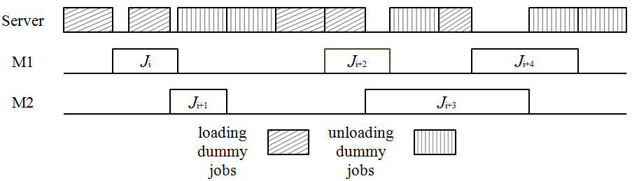
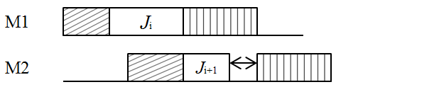
A dummy-job representation (see Elidrissi et al. [2021]) is used in this paper to simplify the problem and make it possible to model the problem as a relatively neat MILP model. Indeed, in our modeling, we consider the single server as the $(m+1)^{th}$ (i.e., third) machine. Each time the server is used to load (resp. unload) job $J_{j}\in\mathcal{N}_{1}$ on machine $k\in M$ , then a dummy job $J_{j+n}\in\mathcal{N}_{2}$ (resp. $J_{j+2n}\in\mathcal{N}_{3}$ ) is processed on the dummy machine $(m+1)$ at the same time. This dummy job $J_{i+n}$ (resp. $J_{i+2n}$ ) has a processing time equal to the loading time (resp. unloading time) of the job $J_{j}$ (i.e., $s_{j}=p_{j+n}$ and $t_{j}=p_{j+2n}$ $\forall j\in\{1,\ldots,n\}$ ) (see Figure 1) . To define the MILP formulations, we adopt the dummy-job representation.

Refer to caption — Figure 1: Dummy-job representation.

3.2 Formulation 1: Completion-time variables

In this section, we propose a completion-time variables formulation $(CF)$ for the problem $P2,S1|s_{j},t_{j}|C_{max}$ . A completion-times variables or disjunctive formulation (see Balas [1985]) has been widely used to model different scheduling problems [Baker and Keller, 2010, Keha et al., 2009, Elidrissi et al., 2022]. In our formulation, we use the following decision variables :

Binary decision variables :

$x_{i,k}=\left\{\begin{array}[]{r l l}1&$ if job $J_{i}$ is processed on machine $k$ $&\\ 0&$otherwise$&\\ \end{array}\right.$

$z_{i,j}=\left\{\begin{array}[]{r l l}1&$ if job $J_{i}$ is processed before job $J_{j}$ $&\\ 0&$otherwise$&\\ \end{array}\right.$

$y_{i+n,j+n}=\left\{\begin{array}[]{r l l}1&$ if the loading dummy job $J_{i+n}$ is processed before the loading dummy $\\ &$ job $J_{j+n}$ on the server $\\ 0&$otherwise$&\\ \end{array}\right.$

$y_{i+2n,j+2n}=\left\{\begin{array}[]{r l l}1&$ if the unloading dummy job $J_{i+2n}$ is processed before the unloading dummy $&\\ &$ job $J_{j+2n}$ on the server $&\\ 0&$otherwise$&\\ \end{array}\right.$

The objective function (1) indicates that the makespan (i.e., the completion time of the last job that finishes its processing on the machines) is to be minimized. Constraint set (13) represents the restriction that the makespan of an optimal schedule is greater than or equal to the completion time of the last executed job. Constraint set (13) states that each job must be processed on exactly one machine. Constraint set (13) ensures that the completion time of each job is at least greater than or equal to the sum of the loading, the unloading and the processing times of this job. In addition, the completion time of each loading dummy job (resp. unloading dummy job) is at least greater than or equal to its loading time (resp. unloading time). Constraint sets (13) and (13) indicate that no two jobs $J_{i}$ and $J_{j}$ , scheduled on the same machine (i.e., $x_{i,k}=x_{j,k}=1$ ), can overlap in time. Constraint sets (13) and (13) state that no two dummy jobs $J_{j+n}$ (resp. $J_{j+2n}$ ) and $J_{i+n}$ (resp. $J_{i+2n}$ ), scheduled on the single server can overlap in time.

$\displaystyle(CF)$	$\displaystyle\min$	$\displaystyle C_{max}$	(1)
	$\displaystyle s.t.$	$\displaystyle C_{max}\geq C_{i}\quad\forall i\in\mathcal{N}_{1}$	(13)
		$\displaystyle\sum_{k\in M}x_{i,k}=1\quad\forall i\in\mathcal{N}_{1}$
		$\displaystyle C_{i}\geq\rho_{i}\quad\forall i\in\mathcal{N}_{1}\cup\mathcal{N}_{2}\cup\mathcal{N}_{3}$
		$\displaystyle C_{i}+\rho_{j}\leq C_{j}+B(3-x_{i,k}-x_{j,k}-z_{i,j})\quad\forall i,j\in N_{1},i\neq j$
		$\displaystyle z_{i,j}+z_{j,i}=1\quad\forall i,j\in\mathcal{N}_{1},i\neq j$
		$\displaystyle C_{i}+\rho_{j}\leq C_{j}+B(1-y_{i,j})\quad\forall i,j\in\mathcal{N}_{2}\cup\mathcal{N}_{3},i\neq j$
		$\displaystyle y_{i,j}+y_{j,i}=1\quad\forall i,j\in\mathcal{N}_{2}\cup N_{3},i\neq j$
		$\displaystyle C_{i}=C_{i+n}+\rho_{i}-\rho_{i+n}\quad\forall i\in\mathcal{N}_{1}$
		$\displaystyle C_{i}=C_{i+2n}\quad\forall i\in\mathcal{N}_{1}$
		$\displaystyle z_{i,j}\in\{0,1\}\quad\forall i\in\mathcal{N}_{1}$
		$\displaystyle x_{i,k}\in\{0,1\}\quad\forall i\in\mathcal{N}_{1},\forall k\in M$
		$\displaystyle y_{i,j}\in\{0,1\}\quad\forall i,j\in\mathcal{N}_{2}\cup\mathcal{N}_{3}$

Constraints (13) calculate the completion time of each job $J_{i}$ . $C_{i}$ is equal to the completion time of the loading operation, $C_{i+n}$ , plus the processing time and the unloading time of the same job (i.e., $\rho_{i}-\rho_{i+n}$ ). Finally, the completion time of the job $J_{i}$ is equal to the completion time of the unloading operation of the same job (13). Constraint sets (13) - (13) define the variables $z_{i,j}$ , $x_{i,k}$ and $y_{i,j}$ as binary ones.

3.3 Strengthening the completion-time variables formulation

We present here two valid inequalities to reduce the time required to solve problem $P2,S1|s_{j},t_{j}|C_{max}$ by the $CF$ formulation.

Proposition 1.

The following constraints are valid for CF formulation.

\displaystyle C_{max}\geq\sum_{j\in\mathcal{N}_{1}}A_{j}x_{j,k}

\displaystyle\forall k\in M

(14)

Proof.

$\sum_{j=1}^{n}~{}A_{j}x_{j,k}$ represents the total work load time of the machine $k$ (idle times are not counted).

It is obvious to see that $C_{max}\geq\sum_{j\in\mathcal{N}_{1}}~{}A_{j}x_{j,k}$ . Hence, inequalities (14) hold.

∎

Since the two machines are identical, Constraints (15) break the symmetry among the machines.

Proposition 2.

The following constraints are valid for the $CF$ formulation.

\displaystyle\sum_{j\in\mathcal{N}_{1},j<i}x_{j,k-1}\geq x_{i,k}

\displaystyle\forall i\in\mathcal{N}_{1},\forall k\in M\setminus\{1\}

(15)

Note that we refer to Eq. (1)-(13) as $CF$ and by considering the set of constraints Eq. (1)-(15) as $CF^{+}$ . A computational comparison between $CF$ and $CF_{1}^{+}$ is conducted in Section 6.

3.4 Formulation 2 : time-indexed variables

In this section, we propose a time-indexed variables formulation $(TIF)$ for the problem $P2,S1|s_{j},t_{j}|C_{max}$ . A time-indexed variables formulation was introduced by Sousa and Wolsey [1992] for the non-preemptive single machine scheduling problem. It has been used to model different scheduling problems (see [Keha et al., 2009, Baker and Keller, 2010, Unlu and Mason, 2010]. This formulation is based on a time discretization. The time is divided into periods $1,2,3,\ldots,T$ , where period $t$ starts at time $t-1$ and ends at time $t$ . The horizon $T$ is an important part of the formulation and its size depends on. Any upper bound ( $UB$ ) can be chosen as $T$ . However, a tighter upper bound is preferable to reduce the problem size as the number of time points is pseudo-polynomial in the size of the input. In our formulation, we choose $T=\sum_{j\in\mathcal{N}_{1}}(A_{j})$ .

The decision variables are defined as follows:

$x_{\{i,t^{\prime}\}}=\left\{\begin{array}[]{r l l}1&$ if job $i$ starts processing at time $t^{\prime}$ $&\\ 0&$otherwise$&\\ \end{array}\right.$

$\displaystyle(TIF)$	$\displaystyle\min$	$\displaystyle C_{max}$	(16)
	$\displaystyle s.t.$	$\displaystyle\sum_{t^{\prime}=0}^{T-\rho_{i}}(t^{\prime}+\rho_{i})x_{\{i,t^{\prime}\}}\leq C_{max}\quad\forall i\in\mathcal{N}_{1}$	(25)
		$\displaystyle\sum_{i\in\mathcal{N}_{1}}\sum_{s=max(0,t^{\prime}-\rho_{i}+1)}^{t^{\prime}}x_{\{i,s\}}\leq 2\quad\forall t^{\prime}\in[0,T]$
		$\displaystyle\sum_{i\in\mathcal{N}_{2}\cup N_{3}}\sum_{s=max(0,t^{\prime}-\rho_{i}+1)}^{t^{\prime}}x_{\{i,s\}}\leq 1\quad\forall t^{\prime}\in[0,T]$
		$\displaystyle\sum_{t^{\prime}=0}^{T-\rho_{i}}x_{\{i,t^{\prime}\}}=1\quad\forall i\in\mathcal{N}_{1}$
		$\displaystyle\sum_{t^{\prime}=0}^{T-\rho_{i}}x_{\{i,t^{\prime}\}}=1\quad\forall i\in\mathcal{N}_{2}$
		$\displaystyle\sum_{t^{\prime}=0}^{T-\rho_{i}}x_{\{i,t^{\prime}\}}=1\quad\forall i\in\mathcal{N}_{3}$
		$\displaystyle x_{\{i,t^{\prime}\}}=x_{\{i+n,t^{\prime}\}}\quad\forall i\in\mathcal{N}_{1},\forall t^{\prime}\in[0,T]$
		$\displaystyle x_{\{i,t^{\prime}\}}=x_{\{i+2n,t^{\prime}+s_{i}+p_{i}\}}\quad\forall i\in\mathcal{N}_{1},\forall t^{\prime}\in[0,T-\rho_{i}]$
		$\displaystyle x_{\{i,t^{\prime}\}}\in\{0,1\}\quad\forall i\in\mathcal{N}_{1},\forall t^{\prime}\in[0,T-\rho_{i}]$

In this formulation, the objective function (16) indicates that the makespan, is to be minimized. Constraint set (25) represents the fact that the makespan of an optimal schedule is greater than or equal to the completion time of all executed jobs, where job $J_{i}$ that starts its loading operation at time point $t$ (i.e., the job for which $x_{i,t^{\prime}}$ = 1) and will finish at time $C_{i}=t+\rho_{i}$ . The completion time of job $J_{i}$ is calculated as $C_{i}=\sum_{t=0}^{T-\rho_{i}}(t^{\prime}+\rho_{i})x_{i,t^{\prime}}$ . The set of constraints (25) specifies that at any given time, at most two jobs can be processed on all machines. Constraints (25) ensure that at any given time, at most one dummy job (loading dummy job or unloading dummy job) can be processed by the server (i.e., the dummy machine). Constraints (25) express that each job $J_{i}$ must start at some time point $t^{\prime}$ in the scheduling horizon, where $t^{\prime}\leq T-s_{i}-p_{i}-t_{i}$ . Constraints (25) state that each loading dummy job must start at some time point $t^{\prime}$ on the dummy machine in the scheduling horizon, where $t^{\prime}\leq T-s_{i}$ . Constraints (25) guarantee that each unloading dummy job must start at some time point $t^{\prime}$ on the dummy machine in the scheduling horizon, where $t^{\prime}\leq T-u_{i}$ . Constraints (25) express that the start time of the loading dummy job $J_{i+n}$ on the dummy machine and the start time of the job $J_{i}$ is the same (i.e. $x_{i,t^{\prime}}=x_{i+n,t^{\prime}}$ ). Constraints (25) ensure that the unloading operation of the job $J_{i}$ starts immediately after the end of the processing operation of the same job (i.e. $x_{i,t^{\prime}}=x_{i+2n,t^{\prime}+s_{i}+p_{i}}$ ). Finally, constraints (25) define the feasibility domain of the decision variables.

3.5 Enhanced time-indexed formulation

We show here how to reduce the number of variables and constraints required by the $TIF$ formulation (16)–(25) and therefore, improving its computational behavior. The size of the $TIF$ formulation depends on the time horizon $T$ . Thus, a reduction of the length of the time horizon is necessary. To do so, we fix the value of $T$ to the approximate makespan solution given by the GVNS metaheuristic presented in Section 5.2. It is clear that the new value of $T$ is less than the upper bound $UB=\sum_{j\in\mathcal{N}_{1}}(A_{j})$ . A comparative study between these two values of $T$ is conducted in the section on computational results (Section 5.2). We refer to $TIF$ with the reduced value of the time horizon $T$ as formulation $TIF^{+}$ .

4 Machines Idle-time property, polynomial-time solvable cases and lower bounds

4.1 Machines Idle-time property

In this section, we show that for the problem $P2,S1|s_{j},t_{j}|C_{max}$ , the minimization of the makespan is equivalent to the minimization of the total idle time of the machines. First, we denote by $\widehat{IT}$ the total idle time of the machines. The machine idle time is the time a machine which has just finished the unloading operation of a job is idle before it starts the loading operation of the next job (we recall that in loading and unloading operations, both the machine and the server are occupied). Indeed, this idle time is due to the unavailability of the server. Note that we include in this definition the Idle-time on a machine after all of its processing is completed, but before the other machine completes its processing (see Koulamas [1996]). In addition, we denote by $IT_{k}$ the total machine idle time in a machine $k$ . Therefore, Proposition 3 and Proposition 4 can be derived.

Proposition 3.

The total idle time of machine $k$ is computed as follows:

IT_{k}=C_{max}-\sum_{j\in\mathcal{N}_{1}}x_{j,k}A_{j}\quad\forall k\in M

(26)

Proposition 4.

The total idle time of the machines is equal to:

\widehat{IT}=mC_{max}-\sum_{j\in\mathcal{N}_{1}}A_{j}

(27)

Proof.

since we have

\sum_{k\in M}x_{j,k}=1\quad\forall j\in\mathcal{N}_{1}

IT_{k}=C_{max}-\sum_{j\in\mathcal{N}_{1}}x_{j,k}(s_{j}+p_{j}+t_{j})\quad\forall k\in M

we obtain

	$\displaystyle\widehat{IT}$	$\displaystyle=\sum_{k\in M}IT_{k}$
		$\displaystyle=\sum_{k\in M}\Big{(}C_{max}-\sum_{j\in\mathcal{N}_{1}}x_{j,k}(s_{j}+p_{j}+t_{j})\Big{)}$
		$\displaystyle=\sum_{k\in M}C_{max}-\sum_{k\in M}\sum_{j\in\mathcal{N}_{1}}x_{j,k}(s_{j}+p_{j}+t_{j})$
		$\displaystyle=\sum_{k\in M}C_{max}-\sum_{j\in\mathcal{N}_{1}}\sum_{k\in M}x_{j,k}(s_{j}+p_{j}+t_{j})$
		$\displaystyle=mC_{max}-\sum_{j\in\mathcal{N}_{1}}(s_{j}+p_{j}+t_{j})$
		$\displaystyle=mC_{max}-\sum_{j\in\mathcal{N}_{1}}A_{j}$

∎

Therefore, for the problem $P2,S1|s_{j},t_{j}|C_{max}$ , the minimization of the makespan is equivalent to the minimization of the total idle time of the machines.

4.2 Polynomial-time solvable cases

We now present some polynomial-time solvable cases for the problem $P2,S1|s_{j},t_{j}|C_{max}$ .

Proposition 5.

We consider a set of jobs, where $s_{i}=p_{j}\quad\forall i,j\in\mathcal{N}_{1}$ and $p_{i}=t_{j}\quad\forall i,j\in\mathcal{N}_{1}$ . Then all permutations define an optimal schedule. In this case, the optimal makespan is equal to the sum of all loading and unloading times of jobs.

Proof.

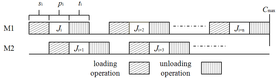
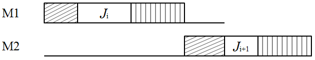
We assume that the processing time of the job scheduled at position 1 is equal to the loading time of the job scheduled at position 2 and the processing time of the job scheduled at position 2 is equal to the unloading time of the job scheduled at position 1. Then, the job at position 2 will start immediately after the end of the loading operation of the job at position 1 and the unloading operation of the job at position 2 will start immediately after the end of the unloading operation of the job at position 1. Therefore, the completion time of the job at position 2 is equal to $C_{[2]}=C_{[1]}+t_{[2]}$ , and the waiting time of the server is equal to 0. Now, if we consider $n$ jobs to be scheduled with $\forall i,j\in\mathcal{N}_{1}\quad s_{i}=p_{j}$ and $\forall i,j\in\mathcal{N}_{1}\quad p_{i}=t_{j}$ , then the jobs will alternate on the two machines, and the total waiting time of the server is equal to zero (see Figure 2). Therefore, in this case all permutations represent an optimal schedule, and the optimal makespan ( $C_{max}^{*}$ ) is equal to the sum of all loading and unloading times (i.e., $C_{max}^{*}=\sum_{j\in\mathcal{N}_{1}}(s_{j}+t_{j})$ ).

∎

Proposition 6.

Consider a set of jobs, where $p_{j}<s_{i}\quad\forall i,j\in\mathcal{N}_{1}$ . Then all permutations define an optimal solution. In this case, the optimal makespan is equal to the sum of the lengths of all jobs ( $C_{max}^{*}=\sum_{j\in\mathcal{N}_{1}}A_{j}$ ).

Proof.

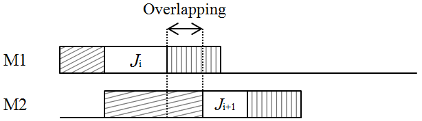
We assume that the processing time of the job scheduled at position 1 is strictly less than the loading time of the job scheduled at position 2. Thus, the job at position 2 cannot be scheduled immediately after the end of the loading operation of the job scheduled at position 1 (see 3a). This is because only one single server is available in the system. Thus, the job at position 2 can be scheduled only after the end of the unloading operation of the job at position 1. In this case, the completion time of the job scheduled at position 2 is equal to $C_{[2]}=C_{[1]}+A_{[2]}$ . Now, if we consider $n$ jobs with $\forall i,j\in\mathcal{N}_{1}\quad p_{j}<s_{j}$ , then each job at position $[i]$ can start its leading operation immediately after the end of the unloading operation of the job scheduled at the position $[i-1]$ . Therefore, in this case all permutations represent an optimal schedule, and the optimal makespan is equal to the sum of all the lengths of the jobs (i.e., $C_{max}^{*}=\sum_{j\in\mathcal{N}_{1}}(A_{j})$ ).

∎

Proposition 7.

Consider a set of jobs, where $s_{i}\leq p_{j}\quad\forall i,j\in\mathcal{N}_{1}$ and $p_{i}<t_{j}\quad\forall i,j\in\mathcal{N}_{1}$ . Then all permutations define an optimal solution. In this case, the optimal makespan is equal to the sum of the lengths of all jobs ( $C_{max}^{*}=\sum_{j\in\mathcal{N}_{1}}A_{j}$ ).

Proof.

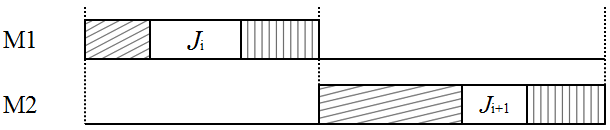
First, we assume that the loading time of the job to be scheduled at position 2 is less than or equal to the processing time of the job scheduled at position 1. Hence, the job to be scheduled at position 2 can start its loading operation in the interval between the end of the loading operation and the start of the unloading operation of the job at position 1. Now, suppose that the processing time of the job at position 2 is strictly less than the unloading time of the job at position 1. Then the job to be scheduled at position 2 can only start its loading operation after the end of the unloading operation of the job at position 1 (see 4b). Therefore, all permutations define an optimal schedule, and the optimal makespan is equal to the sum of the lengths of all jobs (i.e., $C_{max}^{*}=\sum_{j\in\mathcal{N}_{1}}(A_{j})$ ).

∎

4.3 Lower bound

We now introduce a theoretical lower bound ( $LB_{T}$ ) on the optimal objective function value of the problem $P2,S1|s_{j},t_{j}|C_{max}$ , namely $LB_{T}=\max(LB_{1},LB_{2})$ , where $LB_{1}$ and $LB_{2}$ are given in Propositions 8 and 9, respectively.

Proposition 8.

LB_{1}=\frac{\min_{j\in\mathcal{N}_{1}}{s_{j}}+\sum_{j\in\mathcal{N}_{1}}A_{j}+\min_{j\in\mathcal{N}_{1}}{t_{j}}}{2}

is a valid lower bound for the problem $P2,S1|s_{j},t_{j}|C_{max}$ .

Proof.

Let $C_{max}^{*}$ denote the objective function value of an optimal schedule of the problem $P2,S1|s_{j},t_{j}|C_{max}$ . If there is no idle time between two consecutive jobs scheduled on the same machine (i.e., the gap between the end of the processing time and the start time of the loading operation of two jobs scheduled on the same machine is equal to zero) in an optimal schedule of the problem $P2,S1|s_{j},t_{j}|C_{max}$ , then $C_{max}^{*}$ will be equal to the sum of all loading times, processing times and unloading times plus $\min_{j\in\mathcal{N}_{1}}{t_{j}}$ and $\min_{j\in\mathcal{N}_{1}}{s_{j}}$ divided by the number of machines $m=2$ . The fact of adding $\min_{j\in\mathcal{N}_{1}}{t_{j}}$ and $\min_{j\in\mathcal{N}_{1}}{s_{j}}$ with all the loading times, processing times and unloading times will constitute the total load to be executed by the two machines. It is then sufficient to divide this charge by $2$ (i.e., two machines) to obtain the aforementioned lower bound.

∎

Proposition 9.

LB_{2}=\sum_{j\in\mathcal{N}_{1}}(A_{j}-p_{j})

is a valid lower bound for the problem $P2,S1|s_{j},t_{j}|C_{max}$ .

Proof.

This lower bound can be easily derived from Proposition 4. ∎

Therefore:

LB_{T}=\max\left(\frac{\min_{j\in\mathcal{N}_{1}}{s_{j}}+\sum_{j\in\mathcal{N}_{1}}A_{j}+\min_{j\in\mathcal{N}_{1}}{t_{j}}}{2},\sum_{j\in\mathcal{N}_{1}}(A_{j}-p_{j})\right)

5 Solution approaches

This section presents the solution methods to solve large-sized instances of the problem $P2,S1|s_{j},t_{j}|C_{max}$ . First, the solution representation and an initial solution based on an iterative improvement procedure in the insertion neighborhood are presented (Section 5.1). Then, two metaheuristics, namely General variable neighborhood search (GVNS) (Section 5.2) and Greedy randomized adaptive search procedures (GRASP) are proposed (Section 28). The solution approaches are evaluated by extensive computational experiments described in Section 6.

5.1 Solution representation and initial solution

A solution of the problem $P2,S1|s_{j},t_{j}|C_{max}$ can be represented as a permutation $\Pi=\{\pi_{1},\ldots,\pi_{k},\ldots,\pi_{n}\}$ of the job set $\mathcal{N}_{1}$ , where $\pi_{k}$ represents the job scheduled at the $k^{th}$ position. Any permutation of jobs is feasible if a particular machine and the single server are available simultaneously. A job at the $k^{th}$ position is scheduled as soon as possible on an available machine taking into account the loading and unloading constraints of the single server. Note that in our problem the loading, processing and unloading operations are not separable.

We now present an iterative improvement procedure based on the insertion neighborhood that is used as initial solution for our suggested GVNS (Section 5.2). This procedure has been successfully used in different scheduling problems (see Ruiz and Stützle [2007, 2008]). In each step, a job $\pi_{k}$ is removed at random from $\Pi$ and then inserted at all possible $n$ positions. The procedure stops if no improvement is found. It is depicted at Algorithm 1. In Section 6, we show the benefit of using the iterative improvement procedure as a solution finding mechanism for the GVNS metaheuristic.

Data: An instance

\Pi

of the problem

P2,S1|s_{j},t_{j}|C_{max}

; number of jobs

n

Result:

\Pi

1 procedure ()

2 while there is no improvement do

3 for $i=1$ to $n$ do

4 Remove a job

\pi_{k}

at random from

\Pi

\Pi^{\prime}:

best permutation obtained by inserting

\pi_{k}

in any possible position in

\Pi

6 if $C_{max}(\Pi^{\prime})<C_{max}(\Pi)$ then

\Pi\leftarrow\Pi^{\prime}

8 end if

10 end for

12 end while

return

\Pi

Algorithm 1 Iterative Improvement Procedure

5.2 General variable neighborhood search

Variable Neighborhood Search (VNS) is a local search based metaheuristic introduced by Mladenović and Hansen [1997]. It aims to generate a solution that is a local optimum with respect to one or several neighborhood structures. VNS has been successfully applied to different scheduling problems (see Todosijević et al. [2016], Chung et al. [2019], Elidrissi et al. [2022], Maecker et al. [2023]). It consists of three main steps: $i)$ Shaking step (diversification), $ii)$ Local Search step (intensification), and $iii)$ Change Neighborhood step (Move or Not).

We notice that VNS has been less used as a solution method for the PMSSS problem. Mainly, the following metaheuristics have been applied to the PMSSS problem: simulated annealing [Kim and Lee, 2012, Hasani et al., 2014b, d, Hamzadayi and Yildiz, 2016, 2017, Bektur and Saraç, 2019]; genetic algorithm [Abdekhodaee et al., 2006, Huang et al., 2010, Hasani et al., 2014d, Hamzadayi and Yildiz, 2017]; tabu search [Kim and Lee, 2012, Hasani et al., 2014c, Bektur and Saraç, 2019, Alharkan et al., 2019]; ant colony optimization [Arnaout, 2017]; geometric particle swarm optimization [Alharkan et al., 2019]; iterative local search [Silva et al., 2019]; and worm optimization [Arnaout, 2021].

In this section, we propose a General VNS (GVNS) which uses a variable neighborhood descent (VND) as a local search [Hansen et al., 2017]. GVNS starts with an initial solution (generated by the iterative improvement procedure or randomly). Then, the shaking procedure and VND are applied to try to improve the current solution. Finally, this procedure continues until all predefined neighborhoods have been explored and a stopping criterion is met (e.g., a time limit). As far as we know, this is the first study in the literature to propose a GVNS for a parallel machine scheduling problem involving a single server.

5.2.1 Neighborhood structures

Three commonly used neighborhood structures in the literature are adapted to the problem $P2,S1|s_{j},t_{j}|C_{max}$ . The first one is an Interchange-based neighborhood, the second one is an Insert-based neighborhood and the last one is a Reverse-based neighborhood. These structures have been widely applied to solve different scheduling problems (see Hasani et al. [2014b, d], Alharkan et al. [2019]).

The neighborhood structures are defined as follows:

•

Interchange( $\Pi$ ) : It consists of selecting a pair of jobs and exchanging their positions. We consider a solution of the problem denoted as $\Pi_{s}=\{\pi_{1}^{s},\ldots,\pi_{k}^{s},\ldots,\pi_{n}^{s}\}$ , and one of its neighbors $\Pi_{t}=\{\pi_{1}^{t},\ldots,\pi_{k}^{t},\ldots,\pi_{n}^{t}\}$ . We fix two different positions ( $a\neq b$ ), and we exchange the jobs scheduled at the two positions (i.e., $\pi_{a}^{t}=\pi_{b}^{s}$ , $\pi_{b}^{s}=\pi_{a}^{t}$ and $\forall x,x\neq(a,b)$ $\pi_{x}^{t}=\pi_{x}^{s}$ ).
•

Reverse( $\Pi$ ) : It consists of all solutions obtained from the solution $\Pi$ reversing a subsequence of $\Pi$ . More precisely, given two jobs $\pi_{a}$ and $\pi_{b}$ , we construct a new sequence by first deleting the connection between $\pi_{a}$ and its successor $\pi_{a+1}$ and the connection between $\pi_{j}$ and its successor $\pi_{b+1}$ . Next, we connect $\pi_{a}$ with $\pi_{b}$ and $\pi_{a+1}$ with $\pi_{b+1}$ .
•

Insert( $\Pi$ ) : It consists of all solutions obtained from the solution $\Pi$ by removing a job and inserting it at another position in the sequence. We consider a solution $\Pi_{s}=\{\pi_{1}^{s},\ldots,\pi_{k}^{s},\ldots,\pi_{n}^{s}\}$ , and one of its neighbors $\Pi_{t}=\{\pi_{1}^{t},\ldots,\pi_{k}^{t},\ldots,\pi_{n}^{t}\}$ . If $a<b$ , $\pi_{a}^{t}=\pi_{b}^{s}$ , $\pi_{a+1}^{t}=\pi_{a}^{s},\ldots,\pi_{b}^{t}=\pi_{b-1}^{s}$ . Otherwise, if $b<a$ , $\pi_{b}^{t}=\pi_{b+1}^{s},\ldots,\pi_{a-1}^{t}=\pi_{a}^{s}$ , $\pi_{a}^{t}=\pi_{b}^{s}$ .

5.2.2 Variable neighborhood descent

We present here the variable neighborhood descent procedure designed for the problem $P2,S1|s_{j},t_{j}|C_{max}$ . It uses the neighborhood structures described in Section 5.2.1. VND has a solution which is a local optimum with respect to the Interchange, Insert and Reverse neighborhood structures. The order in which the neighborhoods are explored and the way how to move from one neighborhood to another one modify the performance of VND. For this problem, after performing preliminary experiments that are not presented here (as they concern minor parameters with respect to the overall approaches), the following settings are proposed. First, we use a basic sequential VND as a strategy to switch from one neighborhood to another one. Second, the following neighborhood structures order is chosen in the VND procedure: $i)$ Interchange, $ii)$ Insert and $iii)$ Reverse. Finally, the first-improvement strategy (stop generating neighbors as soon as a current solution can be improved in terms of quality) turns out to be better than the best-improvement strategy (generate all the neighbors and choose the best one). The overall VND pseudo-code is presented in Algorithm 2.

Data: A sequence

\Pi

Result:

\Pi

1 procedure Basic_Sequential_VND()

2 repeat

l\leftarrow 1

;

4 while $l\leq 3$ do

5 switch $l$ do

6 case $l=1$ do

\Pi^{\prime}\leftarrow\textsc{interchange}(\Pi)

;

8 break;

9 end case

10 case $l=2$ do

\Pi^{\prime}\leftarrow\textsc{insert}(\Pi)

;

12 break;

13 end case

14 case $l=3$ do

\Pi^{\prime}\leftarrow\textsc{reverse}(\Pi)

;

16 break;

17 end case

19 end switch

l\leftarrow l+1

;

21 if $C_{max}(\Pi^{\prime})<C_{max}(\Pi)$ then

\Pi\leftarrow\Pi^{\prime}

;

l\leftarrow 1

;

25 end if

27 end while

29 until there is no improvement

return

\Pi

;

Algorithm 2 Sequential VND

5.2.3 The proposed GVNS and shaking procedure

To escape from the local optima and have a chance to obtain a global optimum, we propose the following shaking procedure depicted in Algorithm 3. This procedure consists of generating $k$ random jumps from the current solution $\Pi^{\prime}$ using the neighborhood structure Reverse (i.e., $k$ random iterations are performed in Reverse). After preliminary experiments, only one neighborhood structure is used (Reverse), and the value of the diversification factor $k$ is chosen as 15, since they offer the best combination between solution quality (i.e., the quality of the obtained solution) and speed (i.e., the time to generate a feasible solution).

The overall pseudo-code of GVNS as it is designed to solve the problem $P2,S1|s_{j},t_{j}|C_{max}$ is depicted in Algorithm 4. After generating an initial solution (Step 1), a shaking procedure is then applied (Step 2). Once the shaking is performed, VND (Algorithm 2) starts exploring the three proposed neighborhood structures (Step 3). Step 2 and Step 3 until a stopping criterion (CPU) is met (the time limit denoted as $t_{max}$ ). Since GVNS is a trajectory-based procedure, starting from an initial solution is needed. In this paper, we compare two variants of GVNS, namely, one starting from the iterative improvement procedure which we denote as GVNS I, and one starting from a random solution which we denote as GVNS II. GVNS I and GVNS II are both compared in Section 6.

Data:

\Pi

k

: diversification parameter

Result:

\Pi

1 procedure Shaking()

2 for $i=1$ to $k$ do

\Pi^{\prime}

: a random solution with respect to the neighborhood structure Reverse;

5 end for

\Pi\leftarrow\Pi^{\prime}

;

9return

\Pi

Algorithm 3 Shaking

Data: A sequence

\Pi

of the problem

P2,S1|s_{j},t_{j}|C_{max}

t_{max}

: time limit,

k_{max}

Result:

\Pi

C_{max}(\Pi)

1 procedure GVNS()

\Pi\leftarrow

Initial Solution();

3 repeat

k\leftarrow 1

;

5 repeat

\Pi^{\prime}\leftarrow

Shaking

(\Pi,k)

;

\Pi^{\prime\prime}\leftarrow

Basic_Sequential_VND(

\Pi^{\prime}

);

8 if $C_{max}(\Pi^{\prime\prime})<C_{max}(\Pi)$ then

\Pi\leftarrow\Pi^{\prime\prime}

;

k\leftarrow 1

;

12 else

k\leftarrow k+1

;

14 end if

17 until $k>k_{max}$

18 until $CPU>t_{max}$

return

\Pi

Algorithm 4 General VNS for the problem

P2,S1|s_{j},t_{j}|C_{max}

5.3 Greedy randomized adaptive search procedures

The Greedy randomized adaptive search procedure (GRASP) is a local search metaheuristic introduced by [Feo and Resende, 1995]. It has been suggested to solve different scheduling problems [Báez et al., 2019, Yepes-Borrero et al., 2020]. Like GVNS, GRASP has two main phases: diversification phase which is based on a greedy randomized construction procedure and an intensification phase based on the use of a local search procedure. Both phases are repeated in every iteration until a stopping criterion is met (e.g., the number of iterations or/and a time limit). In this section, we propose a hybridization of the GRASP metaheuristic with the VND procedure for the problem $P2,S1|s_{j},t_{j}|C_{max}$ . Indeed, VND is used as a local search method (as it contributes to a significant improvement of the quality of solutions in the preliminary experiments). The overall pseudo-code of our designed GRASP with VND as a local search is presented in the following (Algorithm 5). To the best of our knowledge, our paper is the first one in the literature implementing a GRASP metaheuristic for a variant of the PMSSS problem.

Data: A sequence

\Pi

of the problem

P2,S1|s_{j},t_{j}|C_{max}

t_{max}

: time limit

Result:

\Pi

1 procedure GRASP()

2 repeat

\Pi^{\prime}\leftarrow

Greedy_Randomized_Construction

(\Pi)

\Pi^{\prime\prime}\leftarrow

Basic_Sequential_VND(

\Pi^{\prime}

)

5 if $C_{max}(\Pi^{\prime\prime})<C_{max}(\Pi)$ then

\Pi\leftarrow\Pi^{\prime\prime}

8 end if

10 until $CPU>t_{max}$

return

\Pi

Algorithm 5 Greedy Randomized Adaptive Search Procedures

5.3.1 Greedy randomized construction

The Greedy randomized construction (GRC) procedure of GRASP is presented in Algorithm 6. A solution $\Pi^{\prime}=\{\pi^{\prime}_{1},\ldots,\pi^{\prime}_{k},\ldots,\pi^{\prime}_{n}\}$ is generated iteratively. Indeed, at each iteration of the GRC procedure, a new job is added. First, all jobs from the initial list $\Pi$ are initially inserted into the Candidate List ( $CL$ ). Then, the incremental cost associated with the incorporation of a job $\pi_{s}$ from $CL$ into the solution under construction is calculated. The incremental cost ( $IC$ ) is calculated taking into account the loading and unloading constraints of the single server. Once the $IC$ of all jobs is calculated, we choose the largest and smallest ones, which are denoted by $\Phi_{max}$ and $\Phi_{min}$ , respectively. A Restrict Candidate List ( $RCL$ ) is then created with the best candidate jobs that satisfy the following Inequality (28).

\Phi(\pi_{s})\leq\Phi_{min}+\alpha(\Phi_{max}-\Phi_{min})\quad\forall\pi_{s}\in CL

(28)

The parameter $\alpha$ controls the amounts of greediness and randomness in the GRC procedure. $\alpha_{g}$ is generated uniformly at random from the interval [0, 1] (a purely random construction corresponds to $\alpha=1$ , whereas the greedy construction corresponds to $\alpha=0$ ). Hence, a job $\pi_{s}$ from $RCL$ is selected and scheduled on the first available machine taking into consideration the loading and unloading operations performed by the single server. Finally, $\pi_{s}$ is removed from $CL$ and added to the output solution $\Pi^{\prime}$ . GRASP stops when all jobs from $CL$ are scheduled on the two available machines. In order to improve the solution generated by the GRC procedure, the VND procedure (Algorithm 2) with the same neighborhood structures as described in Section 5.2.2 is used. The stopping criterion of GRASP is the CPU time limit $t_{max}$ .

Data: A job sequence

\Pi

Result:

\Pi^{\prime}

1 procedure Greedy_Randomized_Construction()

2 Initialization:

\Pi^{\prime}\leftarrow\varnothing

\alpha_{g}\in[0,1]

CL\leftarrow\Pi

;

3 Evaluate the incremental cost

\Phi(\pi_{k})

of each job

\pi_{k}\in CL

;

4 repeat

5 Calculate

\Phi_{min}=\min_{\pi_{k}\in CL}\Phi(\pi_{k})

;

6 Calculate

\Phi_{max}=\max_{\pi_{k}\in CL}\Phi(\pi_{k})

;

7 RCL

\leftarrow\{\pi_{j}\in CL|\Phi(\pi_{j})\leq\Phi_{min}+\alpha(\Phi_{max}-\Phi_{min})\}

;

8 Select a job

\pi_{s}

from the RCL list at random;

9 Schedule the selected job

\pi_{s}

on the first available machine at the earliest possible time;

CL\leftarrow CL\setminus\{\pi_{s}\}

;

\Pi^{\prime}\leftarrow\Pi^{\prime}\cup\{\pi_{s}\}

;

12 Reevaluate the incremental cost

\Phi(\pi_{k})

for each remaining job

\pi_{k}\in CL

;

14 until $CL=\varnothing$

return

\Pi^{\prime}

Algorithm 6 Greedy Randomized Construction

6 Computational experiments

This section evaluates the computational performance of the mathematical formulations and the metaheuristic approaches. First, the characteristics of the test instances are provided (Section 6.1). The performance of the mathematical formulations is presented and discussed in Section 6.2. Finally, the performance of the metaheuristic approaches is summarized and discussed in Section 6.3. The computational experiments were conducted on a personal computer Intel(R) Core(TM) with i7-4600M 2.90 GHz CPU and 16GB of RAM, running Windows 7. To solve the $CF$ , $CF^{+}$ , $TIF$ , and $TIF^{+}$ formulations, we have used the Concert Technology library of CPLEX 12.6 version with default settings in C++. The time limit for solving the formulations was set to 3600 s. The meheuristics GVNS I, GVNS II, and GRASP were implemented in the C++ language. We recall that in the proposed GVNS I, the initial solution is obtained using an iterative improvement procedure. In addition, in GVNS II the initial solution is randomly generated. For the proposed GVNS I, GVNS II and GRASP, the time limit ( $t_{max}$ ) is set to 10 seconds for small-sized instances ( $n\in\{8,10,12,25\}$ ), $t_{max}$ is set to 100 seconds for medium-sized instances ( $n\in\{50,100\}$ ), and $t_{max}$ is set to 300 seconds for large-sized instances ( $n\in\{250,500\}$ ). According to the best practice of the related literature, the metaheuristics were executed 10 times in all experiments, except for the small-sized instances for which one run is sufficient, and the best and average results are provided.

6.1 Benchmark instances

To the best of our knowledge, there are no publicly available benchmark instances for the problem $P2,S1|s_{j},t_{j}|C_{max}$ involving a single server for the loading and unloading operations. Therefore, we have generated a set of instances according to the recent literature, as proposed by Kim and Lee [2021] and Lee and Kim [2021].

The instances are characterized by the following features:

•

The number of jobs $n\in\{8,10,12,25,50,100,250,500\}$ .
•

The integer processing times $p_{j}$ are uniformly distributed in the interval [10, 100].
•

The integer loading times $s_{j}=\alpha\times p_{j}$ ( $\alpha\in\{\alpha_{1},\alpha_{2},\alpha_{3}\}$ ), where $\alpha$ is a coefficient randomly generated by the uniform distribution with $\alpha_{1}\in[0.01,0.1]$ , $\alpha_{2}\in[0.1,0.2]$ , and $\alpha_{3}\in[0.1,0.5]$ .
•

The integer unloading times $t_{j}=\alpha\times p_{j}$ .

Note that $\alpha_{1}$ , $\alpha_{2}$ , and $\alpha_{3}$ , respectively, correspond to small, moderate, and large loading/unloading times variance (see Kim and Lee [2021], Lee and Kim [2021]). For each combination of $(n,\alpha_{i})$ $\forall i\in\{1,\ldots,3\}$ , ten instances were created, resulting in a total of 240 new instances. We recall that small-sized instances are those with $n\in\{8,10,12,25\}$ , medium-sized instances are those with $n\in\{50,100\}$ and large-sized instances are those with $n\in\{250,500\}$ .

6.2 Exact approaches

In Table 2, we compare the performance of the $CV$ , $CV^{+}$ , $TIF$ and $TIF^{+}$ formulations for small and medium-sized instances. Note that the results for large-sized instances $n\in\{250,500\}$ are not reported, since all formulations are not able to produce a feasible solution within the time limit of 3600 s. The results are provided for each number $n$ of jobs and for each loading/unloading times variance ( $\alpha\in\{\alpha_{1},\alpha_{2},\alpha_{3}\}$ ). In addition, for each formulation, the following information is given: $i)$ the number of instances solved to optimality, $\#opt$ ; $ii)$ the average time required to obtain an optimal solution, $t(s)$ ; $iii)$ the number of instances with a feasible solution, $\#is$ ; and $iv)$ the average percentage gap to optimality, $gap_{LB}(\%)$ .

Table 2: Comparison of

CF

CF^{+}

TIF

, and

TIF^{+}

for

n\in\{8,10,12,25,50,100\}

Instances		$CF$			$CF^{+}$			$TIF$			$TIF^{+}$
$n$	$\alpha$	$\#opt$	$t(s)$	$\#is$ [ $gap_{LB}(\%)$ ]	$\#opt$	$t(s)$	$\#is$ [ $gap_{LB}(\%)$ ]	$\#opt$	$t(s)$	$\#is$ [ $gap_{LB}(\%)$ ]	$\#opt$	$t(s)$	$\#is$ [ $gap_{LB}(\%)$ ]
8	$\alpha_{1}$	10	6.47	0 [0]	10	0.53	0 [0]	10	4.35	0 [0]	10	3.26	0 [0]
	$\alpha_{1}$	10	5.84	0 [0]	10	0.74	0 [0]	10	12.81	0 [0]	10	7.09	0 [0]
	$\alpha_{1}$	10	4.92	0 [0]	10	0.87	0 [0]	10	36.86	0 [0]	10	11.21	0 [0]
10	$\alpha_{1}$	10	880.51	0 [0]	10	6.58	0 [0]	10	15.09	0 [0]	10	6.81	0 [0]
	$\alpha_{1}$	10	166.43	0 [0]	10	40.07	0 [0]	10	28.64	0 [0]	10	13.83	0 [0]
	$\alpha_{1}$	10	85.68	0 [0]	10	10.70	0 [0]	10	97.43	0 [0]	10	40.66	0 [0]
12	$\alpha_{1}$	0	3600	10 [14.74]	8	1648.67	2 [0.29]	10	51.74	0 [0]	10	12.4	0 [0]
	$\alpha_{1}$	0	3600	10 [18.34]	8	1666.33	2 [0.18]	10	160.67	0 [0]	10	44.74	0 [0]
	$\alpha_{1}$	4	1469.49	6 [20.02]	7	893.33	3 [0.69]	10	555.21	0 [0]	10	149.91	0 [0]
25	$\alpha_{1}$	0	3600	10 [81.39]	0	3600	10 [0.16]	4	2462.14	6 [37.69]	6	1717.90	4 [24.72]
	$\alpha_{1}$	0	3600	9 [77.37]	0	3600	10 [0.26]	1	3537	9 [36.89]	1	2456.37	9 [31.23]
	$\alpha_{1}$	0	3600	1 [66.66]	0	3600	10 [0.91]	0	3600	10 [42.10]	0	3600	10 [38.26]
50	$\alpha_{1}$	0	3600	10 [91.79]	0	3600	10 [0.26]	0	3600	10 [66.46]	0	3600	10 [52.03]
	$\alpha_{1}$	0	3600	9 [91.53]	0	3600	10 [0.60]	0	3600	10 [71.87]	0	3600	10 [58.81]
	$\alpha_{1}$	0	3600	10 [90.36]	0	3600	10 [3.40]	0	3600	10 [73.41]	0	3600	10 [55.26]
100	$\alpha_{1}$	*	*	*	0	3600	10 [0.96]	0	3600	10 [79.63]	0	3600	10 [94.90]
	$\alpha_{1}$	*	*	*	0	3600	10 [3.79]	*	*	*	0	3600	10 [99.98]
	$\alpha_{1}$	*	*	*	0	3600	6 [15.15]	*	*	*	0	3600	10 [100.00]

The following observations can be made:

•

For $n=8$ : Based on the formulations $CF$ , $CF^{+}$ , $TIF$ and $TIF^{+}$ , CPLEX is able to find an optimal solution for any instance. It can be noticed that for the improved formulations $CV^{+}$ and $TIF^{+}$ , CPLEX is able to produce an optimal solution in significantly less computational time in comparison with the original formulation. The best overall performance is demonstrated by $CF^{+}$ with an average computational time required to find an optimal solution equal to 0.71 s.
•

For $n=10$ : For all formulations, CPLEX is able to find an optimal solution for any instance. The best overall performance is demonstrated by $CF^{+}$ for $\alpha_{1}$ , $TIF^{+}$ for $\alpha_{2}$ , and $CF^{+}$ for $\alpha_{3}$ . Based on the formulation $CF^{+}$ , CPLEX is able to produce an optimal solution in significantly less computational time in comparison with $CF$ . The best overall performance is demonstrated by $CF^{+}$ with an average computational time required to find an optimal solution equal to 19.11 s.
•

For $n=12$ : $TIF$ and $TIF^{+}$ are the only formulations for which CPLEX is able to find an optimal solution for any instance. Based on the formulation $CF$ , CPLEX is able to produce an optimal solution for only 4 instances (among 30 ones). In addition, based on the improved formulation $CF^{+}$ , CPLEX is able to find an optimal solution for 24 instances (among 30 ones). Note that the improved formulation $CF^{+}$ reduced significantly the value of $gap_{LB}(\%)$ . The best overall performance is demonstrated by $TIF^{+}$ with an average computational time required to find an optimal solution equal to 69.01 s.
•

For $n=25$ : $TIF^{+}$ is the only formulation for which CPLEX is able to find an optimal solution for 6 instances for $\alpha_{1}$ , and 1 instance for $\alpha_{2}$ . In addition, based on the formulations $CF$ and $CF^{+}$ , CPLEX is able to produce a feasible solution for any instance at best. It can be noticed that the improved formulation $CF^{+}$ reduced significantly the value of $gap_{LB}(\%)$ as compared with the original one. The best overall performance is demonstrated by $TIF^{+}$ .
•

For $n=50$ : For all formulations, CPLEX is able to find a feasible solution for any instance at best. The improved formulations $CF^{+}$ reduced significantly the value of $gap_{LB}(\%)$ . Note that based on the formulation $CF$ , CPLEX is not able to find a feasible solution for 1 instance. The best overall performance is demonstrated by $CF^{+}$ with small values of $gap_{LB}(\%)$ .
•

For $n=100$ : Based on the formulation $CF$ , CPLEX is not able to produce a feasible solution for any instance. Based on formulation $CF^{+}$ , CPLEX is able to find a feasible solution for 26 instances for $\alpha_{3}$ (among the 30 ones). In addition, based on formulation $TIF$ , CPLEX is not able to find a feasible solution for all instances for $\alpha_{2}$ and $\alpha_{3}$ . It can be noticed that the improved formulations $CF^{+}$ reduced significantly the value of $gap_{LB}(\%)$ .

To sum up, the computational comparison of $CF$ , $CF^{+}$ , $TIF$ and $TIF^{+}$ shows that their performance is related to the number of jobs and the loading/unloading times variance. In addition, using the proposed strengthening constraints (14) and (15), the $CF^{+}$ formulation produced lower bounds better than all other formulations for all instances (instances with a feasible solution). Moreover, for $n\in\{8,10\}$ , the best formulation in terms of the average computing time required to obtain an optimal solution is $CF^{+}$ . For $n=12$ , the best performance is demonstrated by $TIF^{+}$ (since it solved to optimality all instances). For $n=25$ , the best performance is demonstrated by $TIF^{+}$ (since it solved 7 instances among the 30 ones to optimality). For $n\in\{50,100\}$ , the best formulation in terms of the average percentage gap to optimality is demonstrated by $CF^{+}$ . It turns out that the formulations $CF^{+}$ and $TIF^{+}$ are complementary. Subsequently, we compare only $CF^{+}$ and $TIF^{+}$ with the other approaches since they produce the best results. Note that $TIF^{+}$ was able to prove optimality within 3600 s for 7 instances among the 30 ones with $n=25$ . Therefore, metaheuristics are needed being able to find an approximate solution in a very short computational time.

6.3 Metaheuristic approaches

6.3.1 Results for small-sized instances

In Tables 3, 4, 5, we compare the performance of $CF^{+}$ , $TIF^{+}$ , GVNS I, GVNS II, and GRASP for instances with $n\in\{8,10,12\}$ , where an optimal solution can be found within 3600 s by $CF^{+}$ and $TIF^{+}$ . Each instance is characterized by the following information. The ID (for example I1 denotes the $1^{th}$ instance with $n=8$ and $\alpha=\alpha_{1}$ ); the number $n$ of jobs; the loading/unloading times variance; the value of the theoretical lower bound $LB_{T}$ computed as in Section 4.3. Next, the optimal makespan (denoted by $C_{max}^{*}$ ) obtained with the $CF^{+}$ and $TIF^{+}$ formulations is given. Finally, the computational time (CPU) to find an optimal solution is given for $CF^{+}$ , $TIF^{+}$ , GVNS I, GVNS II, and GRASP. Note that after each 10 instances of Table 3, 4, 5 (for example I1, $\ldots$ ,I10), the average results for each column are reported (the best results are indicated in bold).

Table 3: Comparison of

CF^{+}

TIF^{+}

, GVNS I, GVNS II, and GRASP in terms of CPU time for

n=8

Instance					$CF^{+}$	$TIF^{+}$	GVNS I	GVNS II	GRASP
ID	$n$	$\alpha$	$LB_{T}$	$C_{max}^{*}$	CPU
I1			295	295	0.456	4.114	0.000	0.001	0.002
I2			288.5	289	0.612	5.486	0.000	0.006	0.054
I3			258.5	259	0.529	4.274	0.000	0.000	0.000
I4			217	217	0.418	2.821	0.006	0.001	0.001
I5	8	$\alpha_{1}$	236.5	237	0.346	2.945	0.000	0.000	0.000
I6			237	238	0.749	3.033	0.000	0.000	0.000
I7			216	218	0.306	2.953	0.001	0.001	0.000
I8			229.5	230	0.629	3.061	0.001	0.000	0.000
I9			193	193	0.731	1.935	0.000	0.001	0.001
I10			194.5	196	0.560	1.942	0.000	0.001	0.001
Avg.			236.55	237.2	0.534	3.256	0.001	0.001	0.006
I11			382.5	383	1.048	9.911	0.013	0.052	0.091
I12			277	277	0.540	5.428	0.002	0.004	0.007
I13			274.5	276	0.561	6.058	0.000	0.004	0.007
I14			326.5	328	0.726	5.673	0.001	0.001	0.000
I15	8	$\alpha_{2}$	259.5	260	0.519	3.853	0.001	0.003	0.001
I16			311.5	312	0.845	6.795	0.000	0.003	0.001
I17			319	320	0.638	10.524	0.003	0.001	0.004
I18			284.5	286	0.831	5.876	0.002	0.003	0.003
I19			334.5	336	0.851	7.455	0.001	0.001	0.001
I20			347	349	0.812	9.326	0.003	0.002	0.001
Avg.			311.65	312.7	0.737	7.090	0.003	0.007	0.011
I21			324	325	0.979	8.029	0.002	0.002	0.080
I22			406.5	408	1.081	10.123	0.127	0.004	8.597
I23			324	325	0.990	15.213	0.006	0.008	0.405
I24			246.5	248	0.634	3.621	0.002	0.016	0.001
I25	8	$\alpha_{3}$	350.5	352	0.839	15.506	0.005	0.004	0.002
I26			331.5	335	0.769	13.742	0.024	0.380	1.893
I27			264.5	266	0.810	3.301	0.002	0.007	0.299
I28			293	300	0.861	25.168	0.000	0.005	0.201
I29			385	387	0.830	9.247	0.008	0.010	0.800
I30			331	331	0.898	8.179	0.005	0.003	0.499
Avg.			325.65	327.70	0.869	11.213	0.018	0.044	1.278

The following observations can be made:

•

In Table 3 : $CF^{+}$ , $TIF^{+}$ , GVNS I, GVNS II, and GRASP are compared. It can be noticed that the three proposed metaheuristics can reach an optimal solution for any instance in significantly less computational time than the two formulations. For example, for $(n=8,\alpha=\alpha_{3}$ ), the average computational time for $CF^{+}$ is 0.869 s, while the average computational time for GVNS I is 0.018 s. It can be noted that the value of the theoretical lower bound ( $LB_{T}$ ) is very tight (since the average gap between the optimal makespan and $LB_{T}$ is equal to 0.427%). The best overall performance is demonstrated by GVNS I with a total average computational time of 0.007 s for $n=8$ .
•

In Table 4 : GVNS I, GVNS II, and GRASP can reach an optimal solution for any instance in significantly less computational time than the $CF^{+}$ and $TIF^{+}$ formulations. For example, for $(n=10,\alpha=\alpha_{1})$ , the average computational time for $TIF^{+}$ is 6.812 s, while the average computational time for GVNS II is equal to 0.003 s. The average gap between $C_{max}^{*}$ and $LB_{T}$ is equal to 0.176%. The best overall performance is shown by GVNS I with a total average computational time of 0.043 s for $n=10$ .
•

In Table 4 : $TIF^{+}$ , GVNS I, GVNS II, and GRASP are compared (since $CF^{+}$ is not able to produce an optimal solution for all instances). It can be noticed that GVNS I, GVNS II, and GRASP can reach an optimal solution for any instance in significantly less computational time than the $TIF^{+}$ formulation. For example, for $(n=12,\alpha=\alpha_{3}$ ), the average computational time for $TIF^{+}$ is equal to 149.914 s, while the average computational time for GVNS I is 2.785 s. Again, the value of $LB_{T}$ is very tight since the average gap between $C_{max}^{*}$ and $LB_{T}$ is equal to 0.115%. The best overall performance is demonstrated by GVNS I with a total average computational time of 0.930 s for $n=10$ .

Table 4: Comparison of

CF^{+}

TIF^{+}

, GVNS I, GVNS II, and GRASP in terms of CPU time for

n=10

Instance					$CF^{+}$	$TIF^{+}$	GVNS I	GVNS II	GRASP
ID	$n$	$\alpha$	$LB_{T}$	$C_{max}^{*}$	CPU
I31			277	277	0.676	4.221	0.006	0.008	0.007
I32			241.5	242	0.716	5.046	0.001	0.001	0.001
I33			310	310	9.827	7.938	0.002	0.004	0.007
I34			298.5	299	1.865	4.864	0.001	0.000	0.001
I35	10	$\alpha_{1}$	312.5	313	1.154	6.523	0.002	0.001	0.001
I36			380	380	17.25	8.272	0.006	0.005	0.001
I37			310.5	311	1.069	8.639	0.001	0.001	0.002
I38			293	293	1.668	10.129	0.005	0.004	0.013
I39			321	321	0.677	9.687	0.039	0.007	0.012
I40			193	193	30.944	2.803	0.001	0.001	0.001
Avg.			293.70	293.90	6.585	6.812	0.006	0.003	0.004
I41			414.5	416	44.247	38.625	0.004	0.008	0.007
I42			445.5	448	14.011	59.407	0.004	0.001	0.002
I43			310	311	9.018	8.268	0.005	0.002	0.002
I44			227	227	0.529	6.365	0.007	0.002	0.010
I45	10	$\alpha_{2}$	347	347	6.84	14.487	0.016	0.044	0.004
I46			222	222	1.981	3.899	0.098	0.002	0.001
I47			316	317	298.729	7.428	0.011	0.036	0.010
I48			280.5	281	1.432	9.469	0.010	0.007	0.007
I49			273	273	12.541	4.958	0.004	0.004	0.013
I50			356.5	357	11.419	15.357	0.006	0.001	0.005
Avg.			319.20	319.90	40.075	16.826	0.016	0.011	0.006
I51			477.5	479	5.491	19.16	0.333	5.346	41.661
I52			316	316	21.075	16.941	0.037	0.515	2.255
I53			518	519	8.023	30.661	0.079	0.063	0.354
I54			456.5	458	17.57	43.689	0.022	0.039	0.051
I55	10	$\alpha_{3}$	411	413	5.638	33.458	0.301	1.459	0.845
I56			347.5	349	7.123	21.732	0.040	0.014	0.034
I57			356.5	358	7.302	25.912	0.114	0.496	0.480
I58			485	487	7.683	67.399	0.023	0.034	0.106
I59			523	523	13.466	92.011	0.022	0.120	0.007
I60			443.5	444	13.581	55.662	0.076	0.552	0.127
Avg.			433.45	434.60	10.695	40.663	0.105	0.864	4.592

Table 5: Comparison of

TIF^{+}

, GVNS I, GVNS II, and GRASP in terms of CPU time for

n=12

Instance					$TIF^{+}$	GVNS I	GVNS II	GRASP
ID	$n$	$\alpha$	$LB_{T}$	$C_{max}^{*}$	CPU
I61			403	403	21.772	0.000	0.000	0.005
I62			338	338	13.471	0.005	0.006	0.003
I63			338.5	339	6.650	0.000	0.002	0.002
I64			330	330	9.110	0.002	0.005	0.002
I65	12	$\alpha_{1}$	393	393	17.890	0.000	0.000	0.005
I66			219.5	220	4.217	0.000	0.000	0.000
I67			352	352	7.460	0.000	0.002	0.002
I68			383	383	12.570	0.002	0.013	0.005
I69			368.5	369	10.415	0.000	0.000	0.002
I70			372	372	20.398	0.002	0.008	0.005
Avg.			349.75	349.9	12.395	0.001	0.003	0.003
I71			474	475	44.769	0.000	0.008	0.002
I72			444.5	446	36.420	0.003	0.000	0.006
I73			459	459	47.066	0.000	0.042	0.014
I74			381	382	18.444	0.003	0.009	0.000
I75	12	$\alpha_{2}$	352.5	353	21.959	0.003	0.000	0.005
I76			500.5	501	64.852	0.016	0.009	0.053
I77			363.5	364	14.919	0.016	0.005	0.006
I78			546.5	547	69.651	0.002	0.000	0.005
I79			589.5	590	105.075	0.006	0.000	0.002
I80			401	402	24.291	0.000	0.000	0.002
Avg.			451.2	451.9	44.745	0.005	0.007	0.009
I81			518	519	150.531	0.480	0.196	0.273
I82			510.5	512	196.291	2.799	3.911	1.894
I83			589.5	590	171.298	2.878	4.770	3.999
I84			684.5	686	213.726	1.797	3.697	4.922
I85	12	$\alpha_{3}$	485.5	486	99.752	1.039	0.013	1.232
I86			570	570	116.832	3.005	1.557	2.717
I87			632	632	207.810	0.187	0.020	0.201
I88			532.5	533	148.399	0.208	0.286	0.614
I89			431	432	46.514	0.925	1.004	1.407
I90			492.5	493	147.986	14.533	52.101	30.002
Avg.			544.60	545.30	149.914	2.785	6.756	4.726

Table 6: Comparison of

CF^{+}

TIF^{+}

, GVNS I, GVNS II and GRASP for

n=25

Instance				$CF^{+}$				$TIF^{+}$				GVNS I			GVNS II			GRASP
ID	$n$	$\alpha$	$LB_{T}$	$UB_{CF^{+}}$	$LB_{CF^{+}}$	$Gap_{CF^{+}}(\%)$	CPU	$UB_{TIF^{+}}$	$LB_{TIF^{+}}$	$Gap_{TIF^{+}}(\%)$	CPU	$C_{max}^{best}$	$C_{max}^{avg}$	CPU	$C_{max}^{best}$	$C_{max}^{avg}$	CPU	$C_{max}^{best}$	$C_{max}^{avg}$	CPU
I91			800.5	801	799.5	0.19	3600	801	549	31.47	3600	801	801	0.03	801	801	0.02	801	801	0.02
I92			763	763	762	0.13	3600	763	763	0	1782.26	763	763	0.16	763	763	0.23	763	763	0.13
I93			860.5	861	859.5	0.17	3600	861	861	0	1454.95	861	861	0.02	861	861	0.01	861	861	0.01
I94			881	882	880	0.23	3600	881	677	23.16	3600	881	881	0.08	881	881	0.10	881	881	0.09
I95	25	$\alpha_{1}$	816	816	815	0.12	3600	816	816	0	970.43	816	816	0.05	816	816	0.07	816	816	0.05
I96			705	705	704	0.14	3600	705	545	22.70	3600	705	705	0.01	705	705	0.01	705	705	0.02
I97			711	711	710	0.14	3600	711	711	0	1189.41	711	711	0.05	711	711	0.03	711	711	0.04
I98			899.5	900	898.5	0.17	3600	901	706.7	21.56	3600	900	900	0.01	900	900	0.01	900	900	0.01
I99			790	790	789	0.13	3600	790	790	0	3025.83	790	790	0.02	790	790	0.02	790	790	0.01
I100			742	742	741	0.13	3600	742	742	0	1884.51	742	742	0.02	742	742	0.02	742	742	0.02
I101			1079.5	1080	1077	0.28	3600	1085	719.6	33.68	3600	1080	1080	0.26	1080	1080	0.20	1080	1080	0.33
I102			997	998	996	0.20	3600	1008	664.9	34.04	3600	997	997	1.65	997	997	1.76	997	997	2.70
I103			767.5	768	766.5	0.20	3600	768	768	0	2456.37	768	768	0.20	768	768	0.18	768	768	0.14
I104			831	832	829.5	0.30	3600	831	586.3	29.45	3600	831	831	0.76	831	831	0.48	831	831	0.81
I105	25	$\alpha_{2}$	854	855	853	0.23	3600	859	573.1	33.28	3600	854	854.2	3.23	854	854.3	2.53	854	854.3	1.99
I106			974.5	975	972.5	0.26	3600	975	650.8	33.25	3600	975	975	0.52	975	975	0.39	975	975	0.58
I107			888	890	887	0.34	3600	891	595	33.22	3600	888	888	1.96	888	888	2.28	888	888	3.28
I108			737.5	739	736.5	0.34	3600	738	558	24.39	3600	738	738	0.20	738	738	0.44	738	738	0.40
I109			978	978	976.5	0.15	3600	988	632.6	35.97	3600	978	978	0.29	978	978	0.24	978	978	0.44
I110			756	757	754.5	0.33	3600	757	576.9	23.79	3600	756	756	1.78	756	756	1.91	756	756	1.84
I111			1023.5	1028	1021	0.68	3600	1052	648.7	38.34	3600	1027	1031.6	5.24	1027	1030.3	6.05	1026	1032.7	3.85
I112			1215	1227	1213	1.14	3600	1250	666.1	46.71	3600	1217	1220.2	4.31	1215	1221.3	4.77	1220	1224.4	5.19
I113			1108	1123	1105.5	1.56	3600	1156	718.4	37.85	3600	1124	1128.1	5.58	1116	1128.8	4.36	1127	1131.7	5.12
I114			1182.5	1187	1179.5	0.63	3600	1255	681.8	45.68	3600	1184	1189.6	5.79	1187	1192.4	5.50	1190	1192.6	4.68
I115	25	$\alpha_{3}$	1216.5	1229	1214.5	1.18	3600	1241	794.5	35.98	3600	1226	1236.1	3.31	1223	1232.8	7.29	1230	1238.7	4.83
I116			1113.5	1123	1110.5	1.11	3600	1141	745.4	34.67	3600	1116	1121.9	5.34	1116	1121.8	6.24	1115	1121.4	5.52
I117			1045	1054	1043	1.04	3600	1074	659.3	38.62	3600	1057	1059.3	4.77	1055	1058	2.92	1050	1055.7	5.55
I118			943	944	941	0.32	3600	953	634.8	33.39	3600	947	951.2	2.96	946	950.8	5.04	946	949.9	6.76
I119			1230.5	1238	1227	0.89	3600	1237	780.9	36.87	3600	1233	1239.5	3.20	1233	1239.6	4.41	1236	1241	5.26
I120			1135	1138	1132	0.53	3600	1159	758.9	34.52	3600	1141	1145.9	3.31	1138	1146.3	5.10	1137	1144.8	4.97

In Table 6, we compare the performance of $CF^{+}$ , $TIF^{+}$ , GVNS I, GVNS II, and GRASP for $n=25$ . Each instance is characterized by the following information. The ID; the number $n$ of jobs; the loading/unloading times variance; and the value of the theoretical lower bound $LB_{T}$ . For the formulation $CF^{+}$ (resp. $TIF^{+}$ ), the following information is given. The upper bound $UB_{{CF}^{+}}$ (respectively $UB_{{TIF}^{+}}$ ), the lower bound $LB_{{CF}^{+}}$ (respectively $LB_{{TIF}^{+}}$ ), the percentage gap to optimality $Gap_{{CF}^{+}}(\%)$ (resp. $Gap_{{TIF}^{+}}(\%)$ ), and the CPU time required to prove optimality (below 3600 s). The following results are presented for GVNS I, GVNS II and GRASP: the best (resp. the average) makespan value over 10 runs denoted as $C_{max}^{best}$ (resp. $C_{max}^{avg}$ ). Finally, the average computational times are also provided that are computed over the 10 runs, and the computational time of a run corresponds to the time at which the best solution is found (the best results are indicated in bold face).

The following observations can be made. Based on $CF^{+}$ , CPLEX is not able to produce an optimal solution for all instances. Furthermore, based on the $TIF^{+}$ formulation, CPLEX is able to find an optimal solution for 6 instances for ( $n=25,\alpha=\alpha_{1}$ ) (I2, I3, I5, I7, I9 and I10). For these instances, GVNS I, GVNS II, and GRASP are able to find the same optimal solution in a significantly less computational time in comparison with $TIF^{+}$ . For ( $n=25,\alpha=\alpha_{2}$ ), based on $TIF^{+}$ formulation, CPLEX is able to generate an optimal solution for only 1 instance (I103). GVNS I, GVNS II, and GRASP are able to find the optimal solution for instance I103 in a significantly less computing time in comparison with $TIF^{+}$ . For $\alpha_{3}$ , $CF^{+}$ produced better upper bounds than $TIF^{+}$ . On average, GVNS I, GVNS II, and GRASP are able to produce approximate solutions of better quality in comparison with the upper bounds generated by the formulations $CF^{+}$ and $TIF^{+}$ . To sum up, for $n=25$ GVNS I, GVNS II, and GRASP have a similar performance. In addition, the difference between $C_{max}^{best}$ and $C_{max}^{avg}$ is very small (often below one unit).

6.3.2 Results for medium-sized instances

In Table 10 in the Appendix, we compare the performance of $CF^{+}$ , $TIF^{+}$ , GVNS I, GVNS II, and GRASP for $n=50$ , and in Table 11, we compare the performance of GVNS I, GVNS II, and GRASP only with $CF^{+}$ (since the $TIF^{+}$ formulation is not able to find a feasible solution for the majority of instances). Tables 10, 11 have the same structure as Table 6, and the best results are indicated in bold face.

The following observations can be made.

•

For $n=50$ : Overall, among the 30 instances, GVNS I found 25 best solutions (83.33%), whereas GVNS II and GRASP found 23 (76.66%) and 20 (66.66%) ones, respectively. It can be noted that the difference between $C_{max}^{best}$ and $C_{max}^{avg}$ is on average very small for GVNS I, GVNS II and GRASP. For the instances with $\alpha_{3}$ , $CF^{+}$ produced better upper bounds than $TIF^{+}$ . On average, GVNS I, GVNS II and GRASP are able to produce approximate solutions of better quality in comparison with the upper bounds generated by the formulations $CF^{+}$ and $TIF^{+}$ . In addition, for all instances of $\alpha_{1}$ and $\alpha_{2}$ , the gap between $C_{max}^{best}$ and $LB_{T}$ is very small for GVNS I, GVNS II and GRASP. The best performance in terms of solution quality and computational time is demonstrated by GVNS I, with 24 best solutions and an overall average computational time of 23.86 s.
•

For $n=100$ : Overall, among the 30 instances, GVNS I found 24 best solutions (80%), whereas GVNS II and GRASP found only 16 (53.33%) and 11 (36.66%) ones, respectively. Based on $CF^{+}$ , CPLEX is able to produce a feasible solution at best for 24 instances (4 instances without a feasible solution). For the instances with $\alpha_{1}$ , the gap between $C_{max}^{best}$ and $LB_{T}$ is very small for GVNS I, GVNS II and GRASP. On average, GVNS I, GVNS II and GRASP are able to produce approximate solutions of better quality in comparison with the upper bounds generated by the formulation $CF^{+}$ . For the instances with $\alpha_{3}$ and for GVNS I, GVNS II and GRASP, the difference between $C_{max}^{best}$ and $C_{max}^{avg}$ grows significantly. The best overall performance is demonstrated by GVNS I, with 24 best solutions and an overall average computational time of 27.31 s.

6.3.3 Results for large-sized instances

Tables 12, 13 describe the performance of GVNS I, GVNS II, and GRASP for large-sized instances. They have the same structure as Table 11, and the best results are indicated in bold face. Note that no mathematical formulation is able to obtain a feasible solution within 3600 s.

The following observations can be made:

•

For $n=250$ : Overall, among the 30 instances, GVNS I found 27 best solutions (90%), whereas GVNS II and GRASP found only 3 (10%) and 1 (3.33%), respectively. For all instances and for GVNS I, GVNS II and GRASP, the difference between $C_{max}^{best}$ and $C_{max}^{avg}$ grows significantly. The average computational time for GVNS I (resp. GVNS II and GRASP) is equal to 113 s (resp. 185.64 and 154.10). The best overall performance is demonstrated by GVNS I with 27 best solutions and an overall average computational time of 113 s.
•

For $n=500$ : Overall, among the 30 instances, GVNS I found 29 best solutions (96.66%), whereas GVNS II and GRASP found only 1 (3.33%) and 0 (0%), respectively. For GVNS I, GVNS II and GRASP, the difference between $C_{max}^{best}$ and $C_{max}^{avg}$ grows significantly especially for the instances with $\alpha_{3}$ . The average computational time for GVNS I (resp. GVNS II and GRASP) is equal to 99.72 s (resp. 225.52 and 218.88). The best overall performance is demonstrated by GVNS I with 29 best solutions and an average computational time of 99.72 s.

To sum up, for small-sized instances, GVNS I, GVNS II and GRASP are able to produce an optimal solution for all instances (among the 120 instances) in significantly less computing time in comparison with $CF^{+}$ and $TIF^{+}$ formulations. For medium and large-sized instances, among the 120 instances, GVNS I found 105 best solutions (87.50%), whereas GVNS II and GRASP found only 43 (35.83%) and 32 (26.66%) ones, respectively. This success can be explained by the quality of the initial solution since the iterative improvement procedure contributes significantly to the minimization of the makespan.

Note that the difference between $C_{max}^{best}$ and $C_{max}^{avg}$ for all methods grows with $n$ and $\alpha$ . These results can lead to the indication that the instances with $\alpha_{3}$ are more difficult to solve in comparison with $\alpha_{1}$ and $\alpha_{2}$ , which is expected since the loading/unloading times variance is large for $\alpha_{3}$ .

6.3.4 Discussion

Table 7 presents the performance of GVNS I, GVNS II, and GRASP in terms of the percentage deviation from the theoretical lower bound ( $Gap_{LB_{T}}(\%)$ ) according to the number of jobs and the loading/unloading variance coefficient. In order to compute each percentage deviation, two values are compared: the value of $LB_{T}$ , and the value of the best approximate makespan obtained over 10 runs by the considered method (see Equation 29).

Gap_{LB_{T}}(\%)=100\times\frac{C_{max}^{best}-LB_{T}}{LB_{T}}

(29)

Table 7: Comparison of GVNS I, GVNS II, and GRASP in terms of percentage deviation from the theoretical lower bound for

n\in\{8,10,12,25,50,100,250,500\}

$n$	$\alpha$	$Gap_{LB_{T}}(\%)$
$n$	$\alpha$	GVNSI	GVNSI	GRASP
8	$\alpha_{1}$	0.29	0.29	0.29
	$\alpha_{2}$	0.34	0.34	0.34
	$\alpha_{3}$	0.66	0.66	0.66
10	$\alpha_{1}$	0.07	0.07	0.07
	$\alpha_{2}$	0.19	0.19	0.19
	$\alpha_{3}$	0.27	0.27	0.27
12	$\alpha_{1}$	0.05	0.05	0.05
	$\alpha_{2}$	0.16	0.16	0.16
	$\alpha_{3}$	0.13	0.13	0.13
25	$\alpha_{1}$	0.02	0.02	0.02
	$\alpha_{2}$	0.02	0.02	0.02
	$\alpha_{3}$	0.54	0.39	0.57
50	$\alpha_{1}$	0.02	0.02	0.02
	$\alpha_{2}$	0.02	0.01	0.02
	$\alpha_{3}$	1.50	1.57	1.80
100	$\alpha_{1}$	0.01	0.01	0.01
	$\alpha_{2}$	0.14	0.15	0.17
	$\alpha_{3}$	2.91	3.80	3.68
250	$\alpha_{1}$	0.03	0.06	0.09
	$\alpha_{2}$	0.35	0.82	0.85
	$\alpha_{3}$	3.70	5.73	6.22
500	$\alpha_{1}$	0.02	0.23	0.21
	$\alpha_{2}$	0.31	1.37	1.34
	$\alpha_{3}$	3.66	7.07	7.31

The average percentage deviation from the theoretical lower bound of GVNS I (respectively GVNS II and GRASP) for the instances with $\alpha_{1}$ and $n\in\{8,10,12,25,50,100,250,500\}$ is equal to 0.06 (respectively 0.09 and 0.10). The average percentage deviation from the theoretical lower bound of GVNS I (resp. GVNS II and GRASP) for the instances with $\alpha_{2}$ and $n\in\{8,10,12,25,50,100,250,500\}$ is equal to 0.19 (respectively 0.38% and 0.39%). Finally, the average percentage deviation from the theoretical lower bound of GVNS I (respectively GVNS II and GRASP) for $\alpha_{3}$ and $n\in\{8,10,12,25,50,100,250,500\}$ is equal to 1.67% (resp. 2.45% and 2.58%). One can see that the average percentage deviation from the theoretical lower bound increases with the increase of the loading/unloading times variance. Indeed, as shown in the preceding section, the instances with a large loading/unloading times variance are more difficult to solve than the other instances (we recall that the difference between $C_{max}^{best}$ and $C_{max}^{avg}$ is very small for $\alpha_{1}$ and $\alpha_{2}$ ). The total average percentage deviation from the theoretical lower bound of GVNS I (respectively GVNS II and GRASP) for all instances is equal to 0.642% (respectively 0.98% and 1.02%). To sum up, we can observe the superiority of GVNS I over GVNS II and GRASP.

Moreover, Table 8 summarizes the performance of GVNS I, GVNS II, and GRASP in terms of the percentage deviation from the best-known solution (the best one over all the runs of all the metaheuristics, and the one obtained by the considered metaheuristic) according to $n$ and $\alpha$ . For each metaheuristic, the following features are given: the minimum value of the percentage deviation over all instance’, Min; the average value of the percentage deviation over all instance’, Avg; and the maximum value of the percentage deviation over all instance’, Max. The last line of the table shows total average results. The results show again that GVNS I based on the iterative improvement procedure as initial-solution finding mechanism, on average, yielded a superior performance in terms of minimum, average and maximum gaps when compared to GVNS II, and GRASP.

Table 8: Percentage deviation from the best known solution for GVNS I, GVNS II, and GRASP.

n	$\alpha$	$Gap_{Dev}(\%)$
n	$\alpha$	GVNS I			GVNS II			GRASP
		Min.	Avg.	Max.	Min.	Avg.	Max.	Min.	Avg.	Max.
8	$\alpha_{1}$	0.00	0.00	0.00	0.00	0.00	0.00	0.00	0.00	0.00
	$\alpha_{2}$	0.00	0.00	0.00	0.00	0.00	0.00	0.00	0.00	0.00
	$\alpha_{3}$	0.00	0.00	0.00	0.00	0.00	0.00	0.00	0.00	0.00
10	$\alpha_{1}$	0.00	0.00	0.00	0.00	0.00	0.00	0.00	0.00	0.00
	$\alpha_{2}$	0.00	0.00	0.00	0.00	0.00	0.00	0.00	0.00	0.00
	$\alpha_{3}$	0.00	0.00	0.00	0.00	0.00	0.00	0.00	0.00	0.00
12	$\alpha_{1}$	0.00	0.00	0.00	0.00	0.00	0.00	0.00	0.00	0.00
	$\alpha_{2}$	0.00	0.00	0.00	0.00	0.00	0.00	0.00	0.00	0.00
	$\alpha_{3}$	0.00	0.00	0.00	0.00	0.00	0.00	0.00	0.00	0.00
25	$\alpha_{1}$	0.00	0.00	0.00	0.00	0.00	0.00	0.00	0.00	0.00
	$\alpha_{2}$	0.00	0.00	0.00	0.00	0.00	0.00	0.00	0.00	0.00
	$\alpha_{3}$	0.00	0.24	0.72	0.00	0.10	0.48	0.00	0.27	0.99
50	$\alpha_{1}$	0.00	0.00	0.00	0.00	0.00	0.00	0.00	0.00	0.00
	$\alpha_{2}$	0.00	0.01	0.06	0.00	0.00	0.00	0.00	0.01	0.06
	$\alpha_{3}$	0.00	0.13	0.61	0.00	0.20	0.66	0.00	0.43	1.26
100	$\alpha_{1}$	0.00	0.00	0.00	0.00	0.00	0.00	0.00	0.00	0.00
	$\alpha_{2}$	0.00	0.04	0.15	0.00	0.05	0.17	0.00	0.08	0.18
	$\alpha_{3}$	0.00	0.00	0.00	0.00	0.87	1.47	0.16	0.75	1.29
250	$\alpha_{1}$	0.00	0.00	0.01	0.00	0.03	0.06	0.04	0.06	0.13
	$\alpha_{2}$	0.00	0.02	0.15	0.22	0.48	0.74	0.00	0.51	0.84
	$\alpha_{3}$	0.00	0.00	0.04	0.00	1.97	3.45	0.91	2.44	3.94
500	$\alpha_{1}$	0.00	0.00	0.00	0.14	0.21	0.29	0.11	0.19	0.25
	$\alpha_{2}$	0.00	0.00	0.00	0.77	1.06	1.40	0.63	1.02	1.27
	$\alpha_{3}$	0.00	0.10	0.96	0.00	3.41	4.32	1.83	3.64	4.80
Avg.		0.00	0.02	0.11	0.05	0.35	0.54	0.15	0.39	0.63

7 Managerial insights

In this section, some managerial insights are presented regarding the investigated problem $P2,S1|s_{j},t_{j}|C_{max}$ . We propose to compare our results with the ones of Benmansour and Sifaleras [2021]. Indeed, Benmansour and Sifaleras [2021] suggested a MILP formulation and a GVNS metaheuristic for the problem $P2,S2|s_{j},t_{j}|C_{max}$ involving two dedicated servers : one for the loading operations and one for the unloading operations. Indeed, in the problem $P2,S2|s_{j},t_{j}|C_{max}$ , each job has to be loaded by a dedicated (loading) server and unloaded by a dedicated (unloading) server, respectively, immediately before and after being processed on one of the two machines, while in the problem $P2,S1|s_{j},t_{j}|C_{max}$ , only one resource (server) is in charge of both the loading and unloading operations. The objective of this section is to show the impact of removing the unloading server on the makespan (i.e., the single server will be in charge of both the loading and unloading operations).

We propose first to improve the mathematical formulation proposed in Benmansour and Sifaleras [2021] denoted by $MIP_{2S}$ by adding the two valid inequalities proposed in Section 3.3. The new obtained formulation is denoted by $MIP_{2S}^{+}$ . Therefore, the formulations $MIP_{2S}$ and $MIP_{2S}^{+}$ are compared with the formulations $CF^{+}$ and $TIF^{+}$ (since they presented a better performance than $CF$ and $TIF$ ). In total, four mathematical formulations are obtained and compared: two formulations regarding the problem $P2,S1|s_{j},t_{j}|C_{max}$ with one single server ( $CF^{+}$ and $TIF^{+}$ ), and two formulations regarding the problem $P2,S2|s_{j},t_{j}|C_{max}$ with two dedicated servers ( $MIP_{2S}$ and $MIP_{2S}^{+}$ ). The computational experiments were conducted using the same computer as described in Section 6. In addition, the time limit for solving the formulations $CF^{+}$ , $TIF^{+}$ , $MIP_{2S}$ , and $MIP_{2S}^{+}$ was set to 3600 s. Note that the four formulations are compared using the same instances as presented in Section 6.1 with up to 25 jobs (since we can obtain a proof of optimality for at least one formulation for each problem). To solve the $CF^{+}$ , $TIF^{+}$ , $MIP_{2S}$ , and $MIP_{2S}^{+}$ formulations, we have used the Concert Technology library of the CPLEX 12.6 version with default settings in C++.

In Table 9, we compare the performance of $CV^{+}$ , $TIF^{+}$ , $MIP_{2S}$ and $MIP_{2S}^{*}$ for $n=8$ . First, each instance is characterized by the following information: the ID; the number $n$ of jobs; the loading/unloading variance coefficient ( $\alpha_{1}$ , $\alpha_{2}$ , and $\alpha_{3}$ ). Next, for each mathematical formulation, the following features are given: $i)$ the optimal makespan solution ( $C_{max}^{*}$ ) and $ii)$ the time required to find an optimal solution (CPU). Finally, the gap between the optimal makespan of the problem with one server and the optimal makespan of the problem with two servers denoted as $Gap_{MI}(\%)$ (calculated in Equation 30) are presented:

Gap_{MI}(\%)=100\times\frac{C_{max}^{*}(1server)-C_{max}^{*}(2servers)}{C_{max}^{*}(2servers)}

(30)

The following observations can be made:

•

Based on the formulations $CV^{+}$ , $TIF^{+}$ , $MIP_{2S}$ and $MIP_{2S}^{*}$ , CPLEX is able to find an optimal solution for any instance. The average computing time for $CV^{+}$ is 0.71 s, and the average computational time for $MIP_{2S}^{*}$ is 0.27 s.
•

All formulations are able to find the same optimal solution for 5 instances (I1, I4, I5, I7 and I24).
•

The average value of $Gap_{MI}(\%)$ is equal to 0.31% for $\alpha_{1}$ , it is equal to 0.76% for $\alpha_{2}$ , and it is equal to 1.45% for $\alpha_{3}$ . Therefore, the value $Gap_{MI}(\%)$ increases for a large loading/unloading times variance.
•

The overall average value of $Gap_{MI}(\%)$ over the 30 instances is equal to 0.84%. It can be noticed that the gap between the two problems is very small and for 5 instances, the same optimal solution is obtained with only one single server.

Table 9: Comparison of

CF^{+}

TIF^{+}

MIP_{2S}^{+}

with

MIP_{2S}

by Benmansour and Sifaleras [2021] for

n=8

	Instance		2 servers				1 server
			$MIP_{2S}$		$MIP_{2S}^{+}$		$CF^{+}$		$TIF^{+}$		$Gap_{MI}(\%)$
ID	$n$	$\alpha$	$C_{max}^{*}$	CPU	$C_{max}^{*}$	CPU	$C_{max}^{*}$	CPU	$C_{max}^{*}$	CPU
I1			295	2.98	295	0.33	295	0.46	295	4.11	0
I2			288	2.19	288	0.29	289	0.61	289	5.49	0.35
I3			258	2.66	258	0.31	259	0.53	259	4.27	0.39
I4			217	2.22	217	0.36	217	0.42	217	2.82	0
I5	8	$\alpha_{1}$	237	2.84	237	0.28	237	0.35	237	2.95	0
I6			236	3.20	236	0.30	238	0.75	238	3.03	0.85
I7			218	4.10	218	0.26	218	0.31	218	2.95	0
I8			229	7.32	229	0.26	230	0.63	230	3.06	0.44
I9			192	1.48	192	0.34	193	0.73	193	1.94	0.52
I10			195	1.82	195	0.45	196	0.56	196	1.94	0.51
I11			376	11.79	376	0.23	383	1.05	383	9.91	1.86
I12			276	1.05	276	0.23	277	0.54	277	5.43	0.36
I13			275	2.82	275	0.32	276	0.56	276	6.06	0.36
I14			325	1.49	325	0.27	328	0.73	328	5.67	0.92
I15	8	$\alpha_{2}$	259	1.14	259	0.24	260	0.52	260	3.85	0.39
I16			310	8.60	310	0.26	312	0.85	312	6.80	0.65
I17			319	2.19	319	0.23	320	0.64	320	10.52	0.31
I18			285	1.06	285	0.25	286	0.83	286	5.88	0.35
I19			333	3.03	333	0.21	336	0.85	336	7.46	0.90
I20			344	1.96	344	0.25	349	0.81	349	9.33	1.45
I21			321	2.27	321	0.26	325	0.98	325	8.03	1.25
I22			397	4.82	397	0.30	408	1.08	408	10.12	2.77
I23			321	5.72	321	0.24	325	0.99	325	15.21	1.25
I24			248	2.07	248	0.22	248	0.63	248	3.62	0
I25	8	$\alpha_{3}$	345	1.78	345	0.24	352	0.84	352	15.51	2.03
I26			329	1.53	329	0.27	335	0.77	335	13.74	1.82
I27			262	1.69	262	0.29	266	0.81	266	3.30	1.53
I28			297	1.03	297	0.27	300	0.86	300	25.17	1.01
I29			381	1.98	381	0.31	387	0.83	387	9.25	1.57
I30			327	2.43	327	0.19	331	0.90	331	8.18	1.22
	Avg.		289.83	3.04	289.83	0.27	292.53	0.71	292.53	7.19	0.84

In Tables 14, 15, 16, we compare the performance of $MIP_{2S}$ , $MIP_{2S}^{+}$ , $CF^{+}$ , $TIF^{+}$ , for $n\in\{10,12,25\}$ . First, each instance is characterized by the following information: the ID; the number $n$ of jobs; the loading/unloading times variance coefficient ( $\alpha_{1}$ , $\alpha_{2}$ , and $\alpha_{3}$ ). Then for each formulation, the following information is given: the upper bound ( $UB_{MIP_{2S}}$ , $UB_{MIP_{2S}^{+}}$ , $UB_{{CF}^{+}}$ , $UB_{{TIF}^{+}}$ ), the lower bound ( $LB_{MIP_{2S}}$ , $LB_{MIP_{2S}^{+}}$ , $LB_{{CF}^{+}}$ , $LB_{{TIF}^{+}}$ ), the percentage gap to optimality ( $Gap_{MIP_{2S}}(\%)$ , $Gap_{MIP_{2S}^{+}}(\%)$ , $Gap_{{CF}^{+}}(\%)$ , $Gap_{{TIF}^{+}}(\%)$ ), and the time required to prove optimality (CPU). Finally, the gap between the optimal makespan of the problem with one server and the optimal makespan of the problem with two servers $Gap_{MI}(\%)$ is given. (In Table 16, $Gap_{MI}(\%)$ is not reported since CPLEX is not able to find an optimal solution for any formulation).

The following observations can be made:

•

For $n=10$ : Based on the formulations $MIP_{2S}^{+}$ , $CF^{+}$ , $TIF^{+}$ , CPLEX is able to find an optimal solution for any instance. Based on the formulation $MIP_{2S}$ , CPLEX is able to produce an optimal solution only for 17 instances among the 30 ones. It can be noted that for the improved formulation $MIP_{2S}^{+}$ , CPLEX is able to produce optimal solutions in less computational time in comparison with the original one. The average CPU time for $MIP_{2S}^{+}$ is equal to 0.33 s, whereas the average CPU time for $CF^{+}$ is equal to 19.12 s. The overall average value of $Gap_{MI}(\%)$ over the 30 instances is equal to 0.62%.
•

For $n=12$ : Based on the formulations $MIP_{2S}^{+}$ and $TIF^{+}$ , CPLEX is able to find an optimal solution for any instance. Based on the formulation $CF^{+}$ , CPLEX is able to produce an optimal solution only for 23 instances among the 30 ones. In addition, CPLEX is not able to produce an optimal solution solution for any instance using the formulation $MIP_{2S}$ . It can be noted that for the improved formulation $MIP_{2S}^{+}$ , CPLEX is able to produce optimal solutions in less computational time in comparison with the original one. The average CPU time for $MIP_{2S}^{+}$ is equal to 0.37 s, whereas the average CPU time for $TIF^{+}$ is equal to 69.02 s. The overall average value of $Gap_{MI}(\%)$ over the 30 instances is equal to 0.61%.
•

For $n=25$ : In the case of 1 server, $TIF^{+}$ is the only formulation for which CPLEX is able to produce an optimal solution for 7 instances among the 30 ones. In the case of 2 servers, $MIP_{2S}^{+}$ is the only formulation for which CPLEX is able to produce an optimal solution for 20 instances among the 30 ones. For $\alpha_{3}$ , using the formulations $MIP_{2S}$ and $MIP_{2S}^{+}$ , CPLEX is not able to produce a feasible solution for all instances (except 1 instance I118). The overall average value of $Gap_{MI}(\%)$ for the instances that can be solved to optimality using $MIP_{2S}^{+}$ and $TIF^{+}$ (I92, I93, I95, I97, I99, I100, and I103) is equal to 0.13%.

As it was shown in the previous Table 9 and in the Tables 14, 15, 16 in the Appendix, the gap between the optimal makespan of the problem with one server and the optimal makespan of the problem with two servers ( $Gap_{MI}(\%)$ ) is very small for almost all small-sized instances with $n\in\{8,10,12,25\}$ . Therefore, the use of an extra resource (unloading server) has a small impact on the reduction of the makespan. It can be noticed that in some cases, the same optimal makespan is obtained using only one single server. Indeed, since the loading, processing and unloading operations are non separable, the waiting time of a machine due to the unavailability of the unloading server will always be significant. To sum up, from a managerial point of view, we indicate to use only one single server for both the loading and unloading operations, which can lead to a significant reduction of costs (e.g., electricity and maintenance) and hence a better preservation of environment.

8 Conclusions

In this paper, the scheduling problem with two identical parallel machines and a single server in charge of loading and unloading operations of jobs was addressed. Each job has to be loaded by a single server immediately before its processing. Once the processing operations finished, each job has to be immediately unloaded by the same server. The objective function considered was the minimization of the makespan. We presented two mixed-integer linear programming (MILP) formulations to model the problem, namely: a completion-time variables formulation $CF$ and a time-indexed formulation $TIF$ , and we proposed sets of inequalities that can be used to improve the $CF$ formulation. We also proposed some polynomial-time solvable cases and a tight lower bound. In addition, we showed that the minimization of the makespan is equivalent to the minimization of the total idle time of the machines.

Since the mathematical formulations were not able to cope with the majority of instances, an efficient General Variable Neighborhood Search metaheuristic (GVNS) with two mechanisms for finding an initial solution (one with an iterative improvement procedure (GVNS I) and one with a random initial solution (GVNS II)), and a Greedy Randomized Adaptive Search Procedures (GRASP) metaheuristic were designed. To validate the performance of the proposed GVNS I, GVNS II and GRASP approaches, exhaustive computational experiments on 240 instances were performed. For small-sized instances with up to 25 jobs, GVNS I, GVNS II and GRASP algorithms outperformed the MILP formulations in terms of the computational time to find an optimal solution. However, for medium and large-sized instances, the GVNS I yielded better results than the other approaches. In particular, the average percentage deviation from the theoretical lower bound was equal to 0.642%. Finally, we presented some managerial insights, and our MILP formulations were compared with the ones of Benmansour and Sifaleras [2021] regarding the problem $P2,S2|s_{j},p_{j}|C_{max}$ involving a dedicated loading server and a dedicated unloading server. It turned out that adding an unloading server (extra resource) contributed less to the reduction of the makespan (since the average percentage deviation of the optimal makespan for the two problems is equal to 0.69% for small-sized instances with up to 12 jobs), and in some cases the same optimal solution can be obtained using only one single server. In future research, it would be interesting to adapt the presented approaches to the more general problem $P,S1|s_{j},t_{j}|C_{max}$ involving an arbitrary number of machines. Further works could also measure the effect of the unloading server on the makespan for the problem $P,S2|s_{j},t_{j}|C_{max}$ .

References

Abdekhodaee et al. [2006] Abdekhodaee AH, Wirth A, Gan HS. Scheduling two parallel machines with a single server: the general case. Computers & Operations Research 2006;33(4):994–1009.
Alharkan et al. [2019] Alharkan I, Saleh M, Ghaleb MA, Kaid H, Farhan A, Almarfadi A. Tabu search and particle swarm optimization algorithms for two identical parallel machines scheduling problem with a single server. Journal of King Saud University-Engineering Sciences 2019;.
Allahverdi and Soroush [2008] Allahverdi A, Soroush H. The significance of reducing setup times/setup costs. European Journal of Operational Research 2008;187(3):978–84.
Arnaout [2017] Arnaout JP. Heuristics for the two-machine scheduling problem with a single server. International Transactions in Operational Research 2017;24(6):1347–55.
Arnaout [2021] Arnaout JP. Worm optimisation algorithm to minimise the makespan for the two-machine scheduling problem with a single server. International Journal of Operational Research 2021;41(2):270–81.
Báez et al. [2019] Báez S, Angel-Bello F, Alvarez A, Melián-Batista B. A hybrid metaheuristic algorithm for a parallel machine scheduling problem with dependent setup times. Computers & Industrial Engineering 2019;131:295–305.
Baker and Keller [2010] Baker KR, Keller B. Solving the single-machine sequencing problem using integer programming. Computers & Industrial Engineering 2010;59(4):730–5.
Balas [1985] Balas E. On the facial structure of scheduling polyhedra. In: Mathematical Programming Essays in Honor of George B. Dantzig Part I. Springer; 1985. p. 179–218.
Bektur and Saraç [2019] Bektur G, Saraç T. A mathematical model and heuristic algorithms for an unrelated parallel machine scheduling problem with sequence-dependent setup times, machine eligibility restrictions and a common server. Computers & Operations Research 2019;103:46–63.
Benmansour and Sifaleras [2021] Benmansour R, Sifaleras A. Scheduling in parallel machines with two servers: the restrictive case. In: Variable Neighborhood Search: 8th International Conference, ICVNS 2021, Abu Dhabi, United Arab Emirates, March 21–25, 2021, Proceedings 8. Springer International Publishing; 2021. p. 71–82.
Chung et al. [2019] Chung T, Gupta JN, Zhao H, Werner F. Minimizing the makespan on two identical parallel machines with mold constraints. Computers & Operations Research 2019;105:141–55.
Elidrissi et al. [2021] Elidrissi A, Benmansour R, Benbrahim M, Duvivier D. Mathematical formulations for the parallel machine scheduling problem with a single server. International Journal of Production Research 2021;59(20):6166–84.
Elidrissi et al. [2022] Elidrissi A, Benmansour R, Sifaleras A. General variable neighborhood search for the parallel machine scheduling problem with two common servers. Optimization Letters 2022;:1–31.
Feo and Resende [1995] Feo TA, Resende MG. Greedy randomized adaptive search procedures. Journal of global optimization 1995;6(2):109–33.
Graham et al. [1979] Graham RL, Lawler EL, Lenstra JK, Kan AR. Optimization and approximation in deterministic sequencing and scheduling: a survey. In: Annals of discrete mathematics. Elsevier; volume 5; 1979. p. 287–326.
Hamzadayi and Yildiz [2016] Hamzadayi A, Yildiz G. Event driven strategy based complete rescheduling approaches for dynamic m identical parallel machines scheduling problem with a common server. Computers & Industrial Engineering 2016;91:66–84.
Hamzadayi and Yildiz [2017] Hamzadayi A, Yildiz G. Modeling and solving static m identical parallel machines scheduling problem with a common server and sequence dependent setup times. Computers & Industrial Engineering 2017;106:287–98.
Hansen et al. [2017] Hansen P, Mladenović N, Todosijević R, Hanafi S. Variable neighborhood search: basics and variants. EURO Journal on Computational Optimization 2017;5(3):423–54.
Hasani et al. [2014a] Hasani K, Kravchenko SA, Werner F. Block models for scheduling jobs on two parallel machines with a single server. Computers & Operations Research 2014a;41:94–7.
Hasani et al. [2014b] Hasani K, Kravchenko SA, Werner F. A hybridization of harmony search and simulated annealing to minimize mean flow time for the two-machine scheduling problem with a single server. Int J Oper Res 2014b;3(1):9–26.
Hasani et al. [2014c] Hasani K, Kravchenko SA, Werner F. Minimising interference for scheduling two parallel machines with a single server. International Journal of Production Research 2014c;52(24):7148–58.
Hasani et al. [2014d] Hasani K, Kravchenko SA, Werner F. Simulated annealing and genetic algorithms for the two-machine scheduling problem with a single server. International Journal of Production Research 2014d;52(13):3778–92.
Hu et al. [2013] Hu J, Zhang Q, Dong J, Jiang Y. Parallel machine scheduling with a single server: Loading and unloading. In: International Conference on Combinatorial Optimization and Applications. Springer; 2013. p. 106–16.
Huang et al. [2010] Huang S, Cai L, Zhang X. Parallel dedicated machine scheduling problem with sequence-dependent setups and a single server. Computers & Industrial Engineering 2010;58(1):165–74.
Jiang et al. [2014] Jiang Y, Wang H, Zhou P. An optimal preemptive algorithm for the single-server parallel-machine scheduling with loading and unloading times. Asia-Pacific Journal of Operational Research 2014;31(05):1450039.
Jiang et al. [2015a] Jiang Y, Yu F, Zhou P, Hu J. Online algorithms for scheduling two parallel machines with a single server. International Transactions in Operational Research 2015a;22(5):913–27.
Jiang et al. [2015b] Jiang Y, Zhang Q, Hu J, Dong J, Ji M. Single-server parallel-machine scheduling with loading and unloading times. Journal of Combinatorial Optimization 2015b;30(2):201–13.
Jiang et al. [2017] Jiang Y, Zhou P, Wang H, Hu J. Scheduling on two parallel machines with two dedicated servers. The ANZIAM Journal 2017;58(3-4):314–23.
Keha et al. [2009] Keha AB, Khowala K, Fowler JW. Mixed integer programming formulations for single machine scheduling problems. Computers & Industrial Engineering 2009;56(1):357–67.
Kim and Lee [2021] Kim HJ, Lee JH. Scheduling uniform parallel dedicated machines with job splitting, sequence-dependent setup times, and multiple servers. Computers & Operations Research 2021;126:105115.
Kim and Lee [2012] Kim MY, Lee YH. Mip models and hybrid algorithm for minimizing the makespan of parallel machines scheduling problem with a single server. Computers & Operations Research 2012;39(11):2457–68.
Koulamas [1996] Koulamas CP. Scheduling two parallel semiautomatic machines to minimize machine interference. Computers & Operations Research 1996;23(10):945–56.
Kramer et al. [2021] Kramer A, Iori M, Lacomme P. Mathematical formulations for scheduling jobs on identical parallel machines with family setup times and total weighted completion time minimization. European Journal of Operational Research 2021;289(3):825–40.
Kravchenko and Werner [1997] Kravchenko SA, Werner F. Parallel machine scheduling problems with a single server. Mathematical and Computer Modelling 1997;26(12):1–11.
Kravchenko and Werner [1998] Kravchenko SA, Werner F. Scheduling on parallel machines with a single and multiple servers. Otto-von-Guericke-Universitat Magdeburg 1998;30(98):1–18.
Lee and Kim [2021] Lee JH, Kim HJ. A heuristic algorithm for identical parallel machine scheduling: splitting jobs, sequence-dependent setup times, and limited setup operators. Flexible Services and Manufacturing Journal 2021;33:992–1026.
Maecker et al. [2023] Maecker S, Shen L, Mönch L. Unrelated parallel machine scheduling with eligibility constraints and delivery times to minimize total weighted tardiness. Computers & Operations Research 2023;149:105999.
Michael [2018] Michael LP. Scheduling: theory, algorithms, and systems. Springer, 2018.
Mladenović and Hansen [1997] Mladenović N, Hansen P. Variable neighborhood search. Computers & operations research 1997;24(11):1097–100.
Ou et al. [2010] Ou J, Qi X, Lee CY. Parallel machine scheduling with multiple unloading servers. Journal of Scheduling 2010;13(3):213–26.
Ruiz and Stützle [2007] Ruiz R, Stützle T. A simple and effective iterated greedy algorithm for the permutation flowshop scheduling problem. European journal of operational research 2007;177(3):2033–49.
Ruiz and Stützle [2008] Ruiz R, Stützle T. An iterated greedy heuristic for the sequence dependent setup times flowshop problem with makespan and weighted tardiness objectives. European Journal of Operational Research 2008;187(3):1143–59.
Silva et al. [2019] Silva JMP, Teixeira E, Subramanian A. Exact and metaheuristic approaches for identical parallel machine scheduling with a common server and sequence-dependent setup times. Journal of the Operational Research Society 2019;:1–15.
Sousa and Wolsey [1992] Sousa JP, Wolsey LA. A time indexed formulation of non-preemptive single machine scheduling problems. Mathematical programming 1992;54(1):353–67.
Todosijević et al. [2016] Todosijević R, Benmansour R, Hanafi S, Mladenović N, Artiba A. Nested general variable neighborhood search for the periodic maintenance problem. European Journal of Operational Research 2016;252(2):385–96.
Unlu and Mason [2010] Unlu Y, Mason SJ. Evaluation of mixed integer programming formulations for non-preemptive parallel machine scheduling problems. Computers & Industrial Engineering 2010;58(4):785–800.
Werner and Kravchenko [2010] Werner F, Kravchenko SA. Scheduling with multiple servers. Automation and Remote Control 2010;71(10):2109–21.
Xie et al. [2012] Xie X, Li Y, Zhou H, Zheng Y. Scheduling parallel machines with a single server. In: Proceedings of 2012 International Conference on Measurement, Information and Control. IEEE; volume 1; 2012. p. 453–6.
Yepes-Borrero et al. [2020] Yepes-Borrero JC, Villa F, Perea F, Caballero-Villalobos JP. Grasp algorithm for the unrelated parallel machine scheduling problem with setup times and additional resources. Expert Systems with Applications 2020;141:112959.

Appendix A Detailed results

Table 10: Comparison of

CF^{+}

TIF^{+}

, GVNS I, GVNS II and GRASP for

n=50

Instance				$CF^{+}$				$TIF^{+}$				GVNS I			GVNS II			GRASP
ID	$n$	$\alpha$	$LB_{T}$	$UB_{CF^{+}}$	$LB_{CF^{+}}$	$Gap_{CF^{+}}(\%)$	CPU	$UB_{TIF^{+}}$	$LB_{TIF^{+}}$	$Gap_{TIF^{+}}(\%)$	CPU	$C_{max}^{best}$	$C_{max}^{avg}$	CPU	$C_{max}^{best}$	$C_{max}^{avg}$	CPU	$C_{max}^{best}$	$C_{max}^{avg}$	CPU
I121			1742.5	1745	1741.5	0.20	3600	1764	911.2	48.35	3600	1743	1743	0.19	1743	1743	0.38	1743	1743	0.19
I122			1558	1563	1557	0.38	3600	1582	874.8	44.70	3600	1558	1558	0.15	1558	1558	0.66	1558	1558	0.39
I123			1659.5	1662	1658.5	0.21	3600	1683	869	48.37	3600	1660	1660	0.12	1660	1660	0.35	1660	1660	0.36
I124			1453	1454	1452	0.14	3600	1482	815.2	45.00	3600	1453	1453	0.30	1453	1453	0.42	1453	1453	0.29
I125	50	$\alpha_{1}$	1627	1634	1626	0.49	3600	1649	851.6	48.36	3600	1627	1627	0.72	1627	1627	0.64	1627	1627	1.25
I126			1664.5	1671	1663.5	0.45	3600	1226628	870.7	99.93	3600	1665	1665	0.22	1665	1665	0.27	1665	1665	0.20
I127			1527	1528	1526	0.13	3600	1553	870.3	43.96	3600	1527	1527	0.18	1527	1527	0.58	1527	1527	0.50
I128			1503.5	1504	1502.5	0.10	3600	1537	857.6	44.20	3600	1504	1504	0.07	1504	1504	0.13	1504	1504	0.18
I129			1698	1699	1697	0.12	3600	1735	889	48.76	3600	1698	1698	1.96	1698	1698	3.23	1698	1698	2.87
I130			1724.5	1730	1723.5	0.38	3600	1759	902.5	48.69	3600	1725	1725	0.08	1725	1725	0.26	1725	1725	0.35
I131			1820.5	1825	1819	0.33	3600	1843	954.2	48.23	3600	1821	1821	22.47	1821	1821	23.73	1821	1821.3	33.17
I132			1980.5	1998	1979.5	0.93	3600	1841388	1038.1	99.94	3600	1981	1981.9	26.68	1981	1981.8	33.72	1981	1982	36.83
I133			1636	1637	1635	0.12	3600	1680	861	48.75	3600	1636	1636.6	25.43	1636	1636.9	23.33	1636	1636.8	45.90
I134			1724.5	1732	1723.5	0.49	3600	1749	906	48.20	3600	1725	1725.2	41.57	1725	1725.6	31.09	1725	1725.8	42.43
I135	50	$\alpha_{2}$	1722	1739	1721	1.04	3600	1761	904	48.67	3600	1722	1722.8	44.52	1722	1723	38.90	1723	1723.1	32.88
I136			1619	1621	1618	0.19	3600	1644	850.4	48.27	3600	1620	1620	20.20	1619	1619.7	33.83	1620	1620.1	24.41
I137			1749	1761	1748	0.74	3600	1393159	918.5	99.93	3600	1749	1749.5	44.27	1749	1749.4	20.54	1749	1749.4	34.38
I138			1754.5	1768	1752.5	0.88	3600	1788	920	48.55	3600	1755	1755.1	31.69	1755	1755	13.08	1755	1755.2	34.82
I139			1462	1474	1461	0.88	3600	1513	771	49.04	3600	1462	1462.6	22.75	1462	1462.5	26.40	1462	1462.5	41.41
I140			1994	2001	1993	0.40	3600	2027	1044.4	48.48	3600	1994	1995.1	24.91	1994	1994.7	33.26	1994	1994.5	41.06
I141			2031	2090	2030	2.87	3600	2094	1068.1	48.99	3600	2058	2068.1	25.90	2063	2070	48.70	2064	2069.6	61.96
I142			1929.5	1977	1928.5	2.45	3600	1777900	1015.2	99.94	3600	1955	1967.9	42.96	1953	1965	32.29	1958	1966	52.15
I143			2289.5	2389	2288	4.23	3600	2341	1200.3	48.73	3600	2324	2352.8	53.18	2328	2347.6	50.41	2344	2352.4	53.89
I144			2127.5	2214	2126	3.97	3600	2452	1118.3	54.39	3600	2159	2178.4	46.19	2146	2173.3	43.45	2173	2181.6	39.35
I145	50	$\alpha_{3}$	2255	2322	2252.5	2.99	3600	2382	1182.3	50.37	3600	2281	2311.7	28.00	2296	2311.4	29.97	2297	2308.3	58.64
I146			1984	2034	1981.5	2.58	3600	2129	1041.4	51.08	3600	1997	2015	48.82	2003	2015.3	53.33	2008	2014.4	39.57
I147			2205	2302	2202.5	4.32	3600	2443	1156.9	52.64	3600	2242	2250.6	47.34	2245	2251.9	38.19	2244	2250.8	45.78
I148			2313.5	2375	2312.5	2.63	3600	2366	1214.4	48.67	3600	2349	2365.1	39.90	2347	2365.9	49.14	2353	2366.1	41.94
I149			2104	2176	2103	3.35	3600	2145	1105.7	48.45	3600	2147	2160.1	37.86	2149	2162.6	37.67	2147	2160.4	70.19
I150			2196	2301	2194.5	4.63	3600	2272	1152.3	49.28	3600	2247	2259.1	37.19	2243	2254.8	49.39	2235	2257.4	62.15

Table 11: Comparison of

CF^{+}

, GVNS I, GVNS II and GRASP for

n=100

Instance				$CF^{+}$				GVNS I			GVNS II			GRASP
ID	$n$	$\alpha$	$LB_{T}$	$UB_{CF^{+}}$	$LB_{CF^{+}}$	$Gap_{CF^{+}}(\%)$	CPU	$C_{max}^{best}$	$C_{max}^{avg}$	CPU	$C_{max}^{best}$	$C_{max}^{avg}$	CPU	$C_{max}^{best}$	$C_{max}^{avg}$	CPU
I151			3296	3309	3295	0.42	3600	3296	3296	12.27	3296	3296	14.88	3296	3296	14.31
I152			3293.5	3325	3292.5	0.98	3600	3294	3294	3.69	3294	3294	6.05	3294	3294	8.22
I153			3349	3399	3348	1.50	3600	3349	3349	22.51	3349	3349	21.44	3349	3349	21.71
I154			3128	3133	3127	0.19	3600	3128	3128	11.03	3128	3128	13.00	3128	3128	13.96
I155	100	$\alpha_{1}$	2840.5	2853	2839.5	0.47	3600	2841	2841	4.53	2841	2841	3.89	2841	2841	5.91
I156			3105.5	3140	3104.5	1.13	3600	3106	3106	7.56	3106	3106	5.39	3106	3106	5.82
I157			3044	3052	3043	0.29	3600	3044	3044	9.01	3044	3044	14.66	3044	3044	13.94
I158			3167	3235	3166	2.13	3600	3167	3167.1	18.28	3167	3167	21.30	3167	3167	11.03
I159			3126.5	3157	3125.5	1.00	3600	3127	3127	7.01	3127	3127	5.40	3127	3127	5.51
I160			3088	3132	3087	1.44	3600	3088	3088.1	19.97	3088	3088	20.61	3088	3088.1	30.69
I161			3580.5	3728	3579.5	3.98	3600	3586	3590.8	54.01	3587	3591.8	40.44	3585	3591.4	48.55
I162			3639	3860	3638	5.75	3600	3644	3650.9	26.92	3646	3651	46.31	3645	3650.5	51.24
I163			3212.5	3285	3211.5	2.24	3600	3220	3222.9	34.46	3217	3222.2	59.64	3218	3223.8	33.83
I164			3372	3451	3371	2.32	3600	3377	3382	32.69	3375	3382.9	54.89	3381	3385.5	40.25
I165	100	$\alpha_{2}$	3576.5	3656	3575.5	2.20	3600	3582	3588.1	37.54	3581	3586.9	48.74	3583	3587.5	64.07
I166			3355.5	3788	3354.5	11.44	3600	3358	3363.9	34.64	3362	3365.3	47.19	3362	3367.2	55.01
I167			3565	3666	3564	2.78	3600	3572	3576.1	38.93	3569	3575.3	36.02	3570	3577	33.46
I168			3344	3448	3343	3.05	3600	3351	3353.2	45.02	3346	3352.3	60.23	3349	3352.5	58.84
I169			3627	3749	3626	3.28	3600	3629	3636.4	47.02	3635	3637.3	31.12	3635	3640.5	42.71
I170			3270	3296	3269	0.82	3600	3272	3278.9	34.82	3275	3280.4	51.30	3274	3281	45.42
I171			4461.5	*	*	*	*	4564	4650.7	23.31	4631	4670.7	61.91	4622	4678.2	54.00
I172			4337	5254	4335.5	17.48	3600	4460	4509.9	34.86	4508	4522.3	56.35	4498	4518.3	58.21
I173			3755.5	*	*	*	*	3855	3898.1	21.28	3871	3902	44.49	3861	3911.7	47.72
I174			4390	4531	4389	3.13	3600	4540	4590.5	48.07	4540	4583.4	46.22	4561	4590.1	59.40
I175	100	$\alpha_{3}$	4144	*	*	*	*	4260	4314	20.84	4318	4340.9	40.58	4298	4342.1	50.20
I176			4608.5	*	*	*	*	4752	4801.3	29.87	4776	4812.6	49.47	4769	4815.6	39.64
I177			4411.5	5093	4410.5	13.40	3600	4570	4616.8	32.81	4625	4645.5	44.56	4601	4650.3	54.33
I178			4384.5	4771	4383.5	8.12	3600	4509	4565	34.10	4526	4562.2	38.27	4553	4576.6	52.03
I179			4152.5	5674	4151.5	26.83	3600	4270	4318.6	23.29	4316	4335.9	42.11	4294	4343.2	40.96
I180			3986	5105	3985	21.94	3600	4093	4159.2	49.02	4143	4164.1	42.89	4146	4177.5	60.32

Table 12: Comparison of GVNS I, GVNS II and GRASP for

n=250

Instance				GVNS I			GVNS II			GRASP
ID	$n$	$\alpha$	$LB_{T}$	$C_{max}^{best}$	$C_{max}^{avg}$	CPU	$C_{max}^{best}$	$C_{max}^{avg}$	CPU	$C_{max}^{best}$	$C_{max}^{avg}$	CPU
I181			7985	7988	7993.9	157.51	7988	7994.4	181.84	7991	7995.5	155.60
I182			8118	8120	8124.7	180.11	8124	8129.2	198.61	8124	8128.4	157.28
I183			8361.5	8364	8369.1	135.30	8366	8371.9	178.68	8370	8374.3	116.51
I184			7941.5	7943	7949.5	151.44	7947	7953.3	133.65	7946	7953.6	121.18
I185	250	$\alpha_{1}$	7812	7812	7820.9	139.86	7813	7821.2	188.11	7822	7825.6	133.99
I186			7925	7930	7933.7	132.45	7929	7935.3	192.06	7933	7937	179.39
I187			8768	8769	8772.8	45.51	8773	8776.5	192.07	8774	8781.6	129.45
I188			8215.5	8218	8224.1	139.55	8220	8227.1	254.57	8222	8227.7	149.58
I189			8350.5	8352	8356.8	84.99	8353	8361.1	121.01	8359	8363.6	132.89
I190			7698.5	7704	7707.1	121.58	7709	7712	123.33	7708	7712.9	175.84
I191			9315.5	9332	9365.4	50.05	9401	9415.8	172.26	9402	9421.5	204.80
I192			9120	9148	9209.8	191.30	9198	9221.2	198.00	9208	9228.6	167.77
I193			9611.5	9652	9699.1	124.61	9685	9707	209.73	9690	9723.9	186.50
I194			8972.5	9001	9055.8	135.90	9056	9077.8	193.12	9065	9081.3	154.83
I195	250	$\alpha_{2}$	9138.5	9174	9234.3	168.61	9195	9227.7	220.72	9195	9246.8	186.97
I196			9239.5	9257	9305.2	48.81	9316	9338.9	167.96	9335	9351.7	103.83
I197			9230	9278	9320.8	140.50	9298	9330.8	146.42	9324	9341.9	148.61
I198			9247.5	9258	9307.8	57.58	9320	9345.2	172.22	9305	9347.1	193.85
I199			9178	9212	9265	118.21	9262	9278.6	200.98	9261	9283.3	207.56
I200			9162	9223	9244.9	173.41	9238	9260.4	208.11	9209	9263.4	163.48
I201			11626.5	12019	12281.6	96.05	12266	12337.9	149.72	12323	12374.2	187.44
I202			11171.5	11491	11756.2	45.78	11888	11930.1	178.71	11869	11944.1	132.79
I203			11095	11417	11667	59.15	11702	11848.7	234.54	11751	11853.1	144.67
I204			11264.5	11874	11958.6	162.26	11869	11971.3	253.40	11977	12033.8	80.53
I205	250	$\alpha_{3}$	11385	11965	12095.2	161.03	11996	12133	220.39	12105	12183.2	168.57
I206			11298.5	11640	11814.5	1.58	11971	12045.4	179.96	11972	12063.9	178.81
I207			11368	11727	11966.7	82.51	12030	12111.2	167.23	12072	12149.9	85.02
I208			11262.5	11562	11826.1	46.11	11919	12001	132.54	12018	12062.1	159.30
I209			11443.5	11962	12160	101.88	12182	12235.7	224.77	12196	12260.2	173.39
I210			11460	11922	12144.9	136.39	12047	12176.9	174.42	12147	12245.4	142.54

Table 13: Comparison of GVNS I, GVNS II and GRASP for

n=500

Instance				GVNS I			GVNS II			GRASP
ID	$n$	$\alpha$	$LB_{T}$	$C_{max}^{best}$	$C_{max}^{avg}$	CPU	$C_{max}^{best}$	$C_{max}^{avg}$	CPU	$C_{max}^{best}$	$C_{max}^{avg}$	CPU
I211			16183	16193	16221.3	95.35	16215	16239.5	219.08	16212	16231.7	229.66
I212			16168.5	16169	16190.7	44.93	16206	16223.2	269.14	16208	16224.4	217.81
I213			16052	16053	16061.5	0.00	16094	16110.3	140.95	16093	16104.6	163.79
I214			16039	16040	16059.9	36.41	16068	16091.9	215.93	16072	16084.6	176.23
I215	500	$\alpha_{1}$	16386.5	16387	16408.9	49.72	16424	16450	240.40	16421	16436.7	210.35
I216			16549	16551	16562	0.00	16586	16605.4	214.22	16570	16599.7	212.29
I217			16123.5	16128	16154.1	106.97	16154	16170.5	280.12	16154	16171.5	215.64
I218			16501.5	16503	16514.1	58.74	16541	16557.5	226.26	16542	16550.6	211.71
I219			16476	16478	16505.6	167.26	16526	16541.1	149.62	16513	16524.7	220.66
I220			16395	16399	16436.5	93.41	16430	16459.6	279.06	16428	16444.8	212.82
I221			18336.5	18391	18521.6	26.58	18614	18659.6	207.13	18591	18649.2	207.35
I222			18452	18479	18719.9	168.25	18737	18794	205.39	18714	18805.3	174.90
I223			18351	18421	18554.5	108.90	18605	18658.8	188.27	18596	18662.1	268.61
I224			18287.5	18352	18527.3	238.02	18541	18627.4	243.43	18468	18589.7	224.05
I225	500	$\alpha_{2}$	18507	18565	18735.6	105.35	18737	18820.3	196.79	18780	18825	176.34
I226			17979.5	18037	18202.2	145.61	18221	18280.20	227.92	18224	18286.3	297.78
I227			18974	19065	19235.3	236.62	19211	19301.10	232.63	19227	19285.3	193.06
I228			18554.5	18613	18733.9	121.78	18798	18857.00	189.89	18801	18848.9	171.66
I229			18235	18273	18477.2	122.11	18467	18521.40	216.95	18462	18550.4	206.81
I230			18619	18676	18739.6	0.00	18891	18932.80	192.21	18899	18925.6	242.40
I231			23731.5	25317	25496.4	129.52	25077	25615.40	253.68	25535	25721.4	204.73
I232			21490.5	22093	22885.5	95.73	23048	23265.20	245.40	22862	23160.9	218.52
I233			22338	23166	24063.5	172.02	24007	24169.80	302.08	23958	24143.5	278.67
I234			23310.5	24229	24902.1	160.24	24880	25142.60	275.73	24970	25184.4	260.70
I235	500	$\alpha_{3}$	23104	23905	24303.2	13.52	24907	25162.40	278.16	25034	25133.4	219.44
I236			22535.5	23253	24055.7	166.31	24199	24376.10	193.90	24167	24312	196.42
I237			21615.5	22336	22953.3	141.24	23132	23298.40	174.15	23264	23450.3	232.60
I238			22629.5	23454	23969.7	47.90	24301	24547.60	240.40	24309	24447.9	271.19
I239			21475.5	22011	22522.5	74.06	22923	23110.90	209.81	23067	23236.9	210.89
I240			22855.5	23611	24153.2	64.92	24519	24670.40	256.98	24396	24781.9	239.34

Table 14: Comparison of

CF^{+}

TIF^{+}

MIP_{2S}^{+}

with

MIP_{2S}

by Benmansour and Sifaleras [2021] for

n=10

	Instance		2 servers								1 server
			$MIP_{2S}$				$MIP_{2S}^{+}$				$CF^{+}$				$TIF^{+}$				$Gap_{MI}(\%)$
ID	$n$	$\alpha$	$UB_{MIP_{2S}}$	$LB_{MIP_{2S}}$	$Gap_{MIP_{2S}}(\%)$	CPU	$UB_{MIP_{2S}^{+}}$	$LB_{MIP_{2S}^{+}}$	$Gap_{MIP_{2S}^{+}}(\%)$	CPU	$UB_{CF^{+}}$	$LB_{CF^{+}}$	$Gap_{CF^{+}}(\%)$	CPU	$UB_{TIF^{+}}$	$LB_{TIF^{+}}$	$Gap_{TIF^{+}}(\%)$	CPU
I31			276	276	0	221.90	276	276	0	0.39	277	277	0	0.68	277	277	0	4.22	0.36
I32			241	232	3.73	3600	241	241	0	0.56	242	242	0	0.72	242	242	0	5.05	0.41
I33			309	301	2.59	3600	309	309	0	0.26	310	310	0	9.83	310	310	0	7.94	0.32
I34			298	294	1.34	3600	298	298	0	0.37	299	299	0	1.87	299	299	0	4.86	0.34
I35	10	$\alpha_{1}$	312	312	0	2349.40	312	312	0	0.27	313	313	0	1.15	313	313	0	6.52	0.32
I36			379	368	2.90	3600	379	379	0	0.26	380	380	0	17.25	380	380	0	8.27	0.26
I37			310	310	0	1554.82	310	310	0	0.31	311	311	0	1.07	311	311	0	8.64	0.32
I38			292	292	0	2414.57	292	292	0	0.24	293	293	0	1.67	293	293	0	10.13	0.34
I39			320	320	0	1029.12	320	320	0	0.28	321	321	0	0.68	321	321	0	9.69	0.31
I40			192	179	6.77	3600	192	192	0	0.23	193	193	0	30.94	193	193	0	2.80	0.52
I41			414	414	0	641.43	414	414	0	0.22	416	416	0	44.25	416	416	0	38.63	0.48
I42			444	434	2.25	3600	444	444	0	0.31	448	448	0	14.01	448	448	0	59.41	0.90
I43			309	309	0	1004.36	309	309	0	0.35	311	311	0	9.02	311	311	0	8.27	0.65
I44			226	226	0	81.07	226	226	0	0.31	227	227	0	0.53	227	227	0	6.37	0.44
I45	10	$\alpha_{2}$	346	346	0	165.86	346	346	0	0.57	347	347	0	6.84	347	347	0	14.49	0.29
I46			221	221	0.01	567.00	221	221	0	0.33	222	222	0	1.98	222	222	0	3.90	0.45
I47			314	311	0.96	3600	314	314	0	0.38	317	317	0	298.73	317	317	0	7.43	0.96
I48			280	280	0.01	712.92	280	280	0	0.33	281	281	0	1.43	281	281	0	9.47	0.36
I49			272	271	0.37	3600	272	272	0	0.42	273	273	0	12.54	273	273	0	4.96	0.37
I50			355	355	0.01	1935.59	355	355	0	0.41	357	357	0	11.42	357	357	0	15.36	0.56
I51			477	477	0	840.29	477	477	0	0.43	479	479	0	5.49	479	479	0	19.16	0.42
I52			313	300	4.15	3600	313	313	0	0.26	316	316	0	21.08	316	316	0	16.94	0.96
I53			515	514	0.19	3600	515	515	0	0.30	519	519	0	8.02	519	519	0	30.66	0.78
I54			451	434	3.77	3600	451	451	0	0.25	458	458	0	17.57	458	458	0	43.69	1.55
I55	10	$\alpha_{3}$	410	410	0	439.66	410	410	0	0.28	413	413	0	5.64	413	413	0	33.46	0.73
I56			345	338	2.03	3600	345	345	0	0.31	349	349	0	7.12	349	349	0	21.73	1.16
I57			356	356	0.00	588.64	356	356	0	0.38	358	358	0	7.30	358	358	0	25.91	0.56
I58			481	481	0	91.85	481	481	0	0.27	487	487	0	7.68	487	487	0	67.40	1.25
I59			518	518	0.01	3264.02	518	518	0	0.41	523	523	0	13.47	523	523	0	92.01	0.97
I60			438	395	9.82	3601	438	438	0	0.30	444	444	0	13.58	444	444	0	55.66	1.37
	Avg.		347.13	342.47	1.36	2156.77	347.13	347.13	0	0.33	349.47	349.47	0	19.12	349.47	349.47	0	21.43	0.62

Table 15: Comparison of

CF^{+}

TIF^{+}

MIP_{2S}^{+}

with

MIP_{2S}

by Benmansour and Sifaleras [2021] for

n=12

	Instance		2 servers								1 server
			$MIP_{2S}$				$MIP_{2S}^{+}$				$CF^{+}$				$TIF^{+}$				$Gap_{MI}(\%)$
ID	$n$	$\alpha$	$UB_{MIP_{2S}}$	$LB_{MIP_{2S}}$	$Gap_{MIP_{2S}}(\%)$	CPU	$UB_{MIP_{2S}^{+}}$	$LB_{MIP_{2S}^{+}}$	$Gap_{MIP_{2S}^{+}}(\%)$	CPU	$UB_{CF^{+}}$	$LB_{CF^{+}}$	$Gap_{CF^{+}}(\%)$	CPU	$UB_{TIF^{+}}$	$LB_{TIF^{+}}$	$Gap_{TIF^{+}}(\%)$	CPU
I61			402	318	20.90	3600	402	402	0	0.21	403	403	0	709.72	403	403	0	21.77	0.25
I62			337	253.1	24.89	3600	337	337	0	0.28	338	338	0	2780.13	338	338	0	13.47	0.30
I63			338	240.2	28.93	3600	338	338	0	0.40	339	339	0	1327.14	339	339	0	6.65	0.30
I64			329	273	17.02	3600	329	329	0	0.40	330	329	0.30	3600	330	330	0	9.11	0.30
I65	12	$\alpha_{1}$	391	278.7	28.71	3600	391	391	0	0.49	393	393	0	1318.60	393	393	0	17.89	0.51
I66			219	135	38.33	3600	219	219	0	0.44	220	220	0	3101.09	220	220	0	4.22	0.46
I67			351	325	7.41	3600	351	351	0	0.27	352	351	0.28	3600	352	352	0	7.46	0.28
I68			382	274.4	28.16	3600	382	382	0	0.27	383	383	0	2033.21	383	383	0	12.57	0.26
I69			367	244.8	33.31	3600	367	367	0	0.46	369	369	0	811.76	369	369	0	10.42	0.54
I70			371	262	29.38	3600	371	371	0	0.35	372	372	0	1107.71	372	372	0	20.40	0.27
I71			472	324.9	31.17	3600	472	472	0	0.32	475	475	0	1933.03	475	475	0	44.77	0.64
I72			444	304	31.53	3600	444	444	0	0.37	446	446	0	1062.03	446	446	0	36.42	0.45
I73			457	299.5	34.46	3600	457	457	0	0.44	459	459	0	1393.99	459	459	0	47.07	0.44
I74			379	271.2	28.44	3600	379	379	0	0.54	382	382	0	1687.02	382	382	0	18.44	0.79
I75	12	$\alpha 2$	351	284.4	18.97	3600	351	351	0	0.33	353	353	0	1490.81	353	353	0	21.96	0.57
I76			496	319.5	35.58	3600	496	496	0	0.39	501	500	0.20	3600	501	501	0	64.85	1.01
I77			362	300	17.13	3600	362	362	0	0.31	364	364	0	1915.16	364	364	0	14.92	0.55
I78			543	327	39.77	3600	543	543	0	0.40	547	547	0	2810.76	547	547	0	69.65	0.74
I79			584	369	36.82	3600	584	584	0	0.40	590	589	0.17	3600	590	590	0	105.08	1.03
I80			400	332	17.00	3600	400	400	0	0.26	402	402	0	1037.85	402	402	0	24.29	0.50
I81			512	306.2	40.19	3600	512	512	0	0.42	519	519	0	1848.72	519	519	0	150.53	1.37
I82			508	398.8	21.50	3600	508	508	0	0.56	512	512	0	459.09	512	512	0	196.29	0.79
I83			587	414	29.47	3600	587	587	0	0.30	590	589.9	0	1538.58	590	590	0	171.30	0.51
I84			680	395	41.91	3600	680	680	0	0.42	686	686	0	1020.65	686	686	0	213.73	0.88
I85	12	$\alpha_{3}$	483	399.5	17.29	3600	483	483	0	0.28	486	486	0	219.78	486	486	0	99.75	0.62
I86			566	388.3	31.40	3600	566	566	0	0.35	570	569	0.18	3600	570	570	0	116.83	0.71
I87			625	397.5	36.39	3600	625	625	0	0.40	632	626	0.95	3600	632	632	0	207.81	1.12
I88			527	372.8	29.26	3600	527	527	0	0.28	533	528	0.94	3600	533	533	0	148.40	1.14
I89			429	270.2	37.03	3600	429	429	0	0.40	432	432	0	949.44	432	432	0	46.51	0.70
I90			491	395	19.55	3600	491	491	0	0.30	493	493	0	217.03	493	493	0	147.99	0.41
	Avg.		446.1	315.77	28.40	3600	446.1	446.1	0.00	0.37	449.03	448.50	0.10	1932.47	449.03	449.03	0	69.02	0.61

Table 16: Comparison of

CF^{+}

TIF^{+}

MIP_{2S}^{+}

with

MIP_{2S}

by Benmansour and Sifaleras [2021] for

n=25

	Instance		2 servers								1 server
			$MIP_{2S}$				$MIP_{2S}^{+}$				$CF^{+}$				$TIF^{+}$
ID	$n$	$\alpha$	$UB_{MIP_{2S}}$	$LB_{MIP_{2S}}$	$Gap_{MIP_{2S}}(\%)$	CPU	$UB_{MIP_{2S}^{+}}$	$LB_{MIP_{2S}^{+}}$	$Gap_{MIP_{2S}^{+}}(\%)$	CPU	$UB_{CF^{+}}$	$LB_{CF^{+}}$	$Gap_{CF^{+}}(\%)$	CPU	$UB_{TIF^{+}}$	$LB_{TIF^{+}}$	$Gap_{TIF^{+}}(\%)$	CPU
I91			800	246	69.25	3600	800	800	0	277.00	801	799.5	0.19	3600	801	549	31.47	3600
I92			762	309	59.45	3600	762	762	0	0.68	763	762	0.13	3600	763	763	0	1782.26
I93			860	303.5	64.71	3600	860	860	0	253.33	861	859.5	0.17	3600	861	861	0	1454.95
I94			880	300	65.91	3600	880	880	0	1.01	882	880	0.23	3600	881	677	23.16	3600
I95	25	$\alpha_{1}$	815	280.5	65.58	3600	815	815	0	0.86	816	815	0.12	3600	816	816	0	970.43
I96			704	240.6	65.83	3600	704	704	0	0.49	705	704	0.14	3600	705	545	22.70	3600
I97			710	275	61.27	3600	710	710	0	1.71	711	710	0.14	3600	711	711	0	1189.41
I98			899	275	69.41	3600	899	899	0	1193.36	900	898.5	0.17	3600	901	706.7	21.56	3600
I99			789	294	62.74	3600	789	789	0	10.56	790	789	0.13	3600	790	790	0	3025.83
I100			741	287.7	61.18	3600	741	741	0	0.52	742	741	0.13	3600	742	742	0	1884.51
I101			*	*	*	*	*	*	*	*	1080	1077	0.28	3600	1085	719.6	33.68	3600
I102			996	349	64.96	3600	996	996	0	0.92	998	996	0.20	3600	1008	664.9	34.04	3600
I103			767	315	58.93	3600	767	767	0	1244.90	768	766.5	0.20	3600	768	768	0	2456.37
I104			830	317.9	61.70	3600	830	830	0	686.88	832	829.5	0.30	3600	831	586.3	29.45	3600
I105	25	$\alpha_{2}$	853	336	60.61	3600	853	853	0	0.69	855	853	0.23	3600	859	573.1	33.28	3600
I106			973	325	66.60	3600	973	973	0	425.89	975	972.5	0.26	3600	975	650.8	33.25	3600
I107			887	373	57.95	3600	887	887	0	1.01	890	887	0.34	3600	891	595	33.22	3600
I108			737	302	59.02	3600	737	737	0	550.15	739	736.5	0.34	3600	738	558	24.39	3600
I109			977	363	62.85	3600	977	977	0	1038.33	978	976.5	0.15	3600	988	632.6	35.97	3600
I110			755	281	62.78	3600	755	755	0	3088.83	757	754.5	0.33	3600	757	576.9	23.79	3600
I111			*	*	*	*	*	*	*	*	1028	1021	0.68	3600	1052	648.7	38.34	3600
I112			*	*	*	*	*	*	*	*	1227	1213	1.14	3600	1250	666.1	46.71	3600
I113			*	*	*	*	*	*	*	*	1123	1105.5	1.56	3600	1156	718.4	37.85	3600
I114			*	*	*	*	*	*	*	*	1187	1179.5	0.63	3600	1255	681.8	45.68	3600
I115	25	$\alpha_{3}$	*	*	*	*	*	*	*	*	1229	1214.5	1.18	3600	1241	794.5	35.98	3600
I116			*	*	*	*	*	*	*	*	1123	1110.5	1.11	3600	1141	745.4	34.67	3600
I117			*	*	*	*	*	*	*	*	1054	1043	1.04	3600	1074	659.3	38.62	3600
I118			941	376	60.042508	3600	941	941	0	0.65	944	941	0.32	3600	953	634.8	33.39	3600
I119			*	*	*	*	*	*	*	*	1238	1227	0.89	3600	1237	780.9	36.87	3600
I120			*	*	*	*	*	*	*	*	1138	1132	0.53	3600	1159	758.9	34.52	3600