SCP: Spherical-Coordinate-Based Learned Point Cloud Compression
Abstract
In recent years, the task of learned point cloud compression has gained prominence. An important type of point cloud, the spinning LiDAR point cloud, is generated by spinning LiDAR on vehicles. This process results in numerous circular shapes and azimuthal angle invariance features within the point clouds. However, these two features have been largely overlooked by previous methodologies. In this paper, we introduce a model-agnostic method called Spherical-Coordinate-based learned Point cloud compression (SCP), designed to leverage the aforementioned features fully. Additionally, we propose a multi-level Octree for SCP to mitigate the reconstruction error for distant areas within the Spherical-coordinate-based Octree. SCP exhibits excellent universality, making it applicable to various learned point cloud compression techniques. Experimental results demonstrate that SCP surpasses previous state-of-the-art methods by up to 29.14% in point-to-point PSNR BD-Rate.
Introduction
LiDAR point clouds play a crucial role in numerous real-world applications, including self-driving vehicles (Li et al. 2020; Fernandes et al. 2021; Silva et al. 2023), robotics (He et al. 2021b, 2020; Wang et al. 2019) and 3D mapping (Choe et al. 2021; Li et al. 2021). However, the transmission and storage of these point clouds present significant challenges. A typical large point cloud may contain up to a million points (Quach, Valenzise, and Dufaux 2019), making direct storage highly inefficient.
In an effort to mitigate the transmission and storage costs associated with point clouds, MPEG introduced a hand-crafted compression standard known as Geometry-based Point Cloud Compression (G-PCC) (ISO/IEC JTC 1/SC 29/WC 7 2021). This standard employs different geometric structures, including the Octree (Jackins and Tanimoto 1980) and predictive geometry (ISO/IEC JTC 1/SC 29/WC 7 2019), to compress point clouds. The Octree-based entropy model is a widely adopted approach in both G-PCC and learned methods for representing and compressing point clouds. Simultaneously, another geometric structure, predictive geometry, capitalizes on the chain structure formed by each LiDAR laser beam. It predicts the position of the next point based on the angles and distances of preceding points on the chain. Other than basic G-PCC, a Cylindrical-coordinate-based method (Sridhara, Pavez, and Ortega 2021) suggests transforming the Cartesian-coordinate positions into Cylindrical coordinates for G-PCC to compress. In the Cylindrical coordinates, when splitting coordinate for Octree construction, points from the same chain (points acquired by the same laser beam) tend to be grouped into the same voxel, as shown in Fig. 1(b)-left. Thus, these points have more relevant information in their context for compressing. Consequently, this method improves the performance of G-PCC. In the meanwhile, Cylinder3D (Zhu et al. 2021) also took the use of Cylindrical coordinates in the point cloud segmentation task. Concurrently, learned point cloud compression methods are emerging, using deep learning techniques to compress point clouds. Former work such as OctSqueeze (Huang et al. 2020), VoxelDNN (Nguyen et al. 2021a), VoxelContext-Net (Que, Lu, and Xu 2021), and OctFormer (Cui et al. 2023) employ information of ancient voxels for prediction of the current one. Advancing these approaches, OctAttention (Fu et al. 2022), SparsePCGC (Wang et al. 2022), and EHEM (Song et al. 2023) harness the voxels in the same level as the current one to minimize the redundancy.
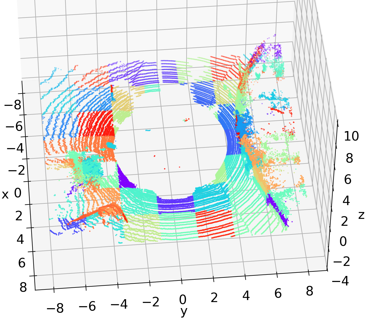
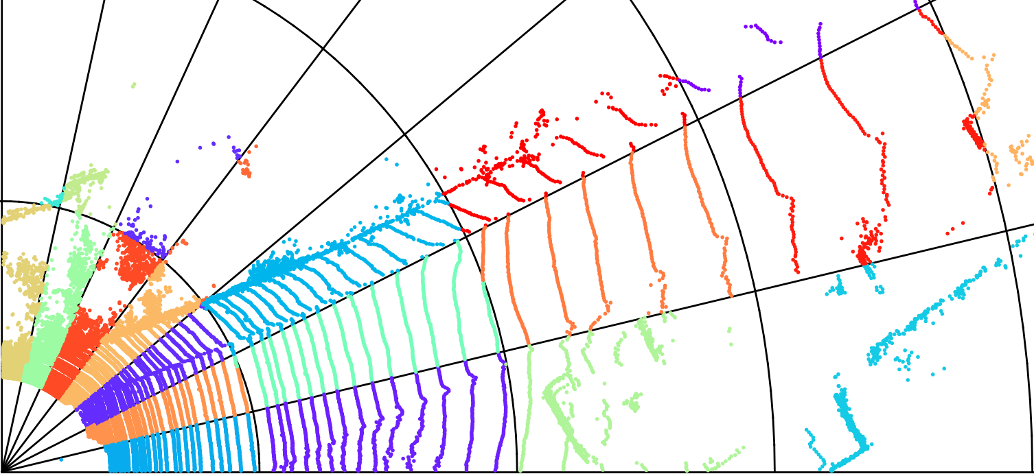
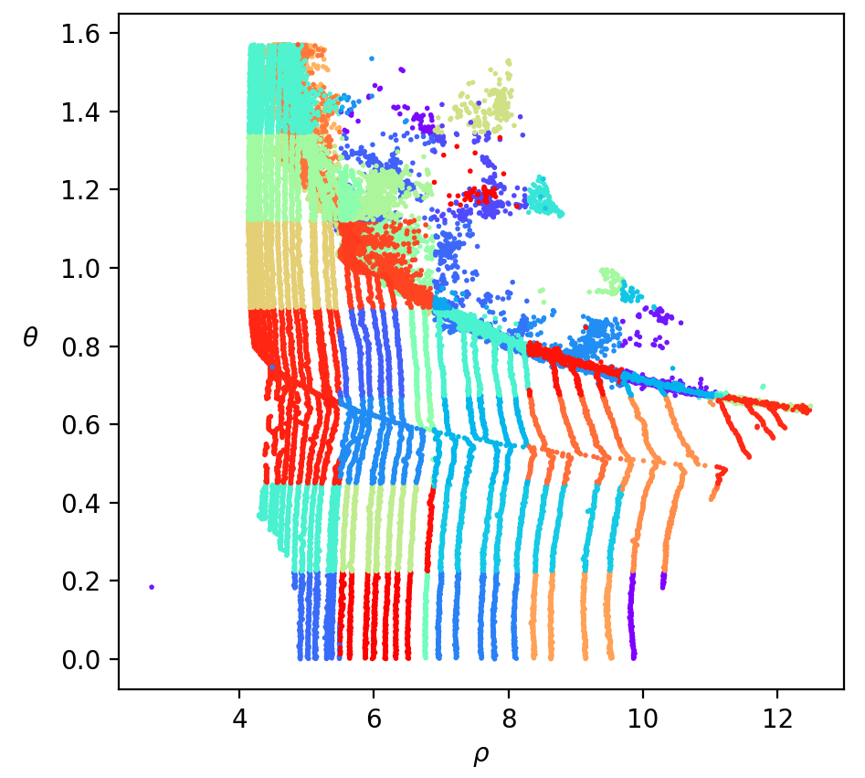
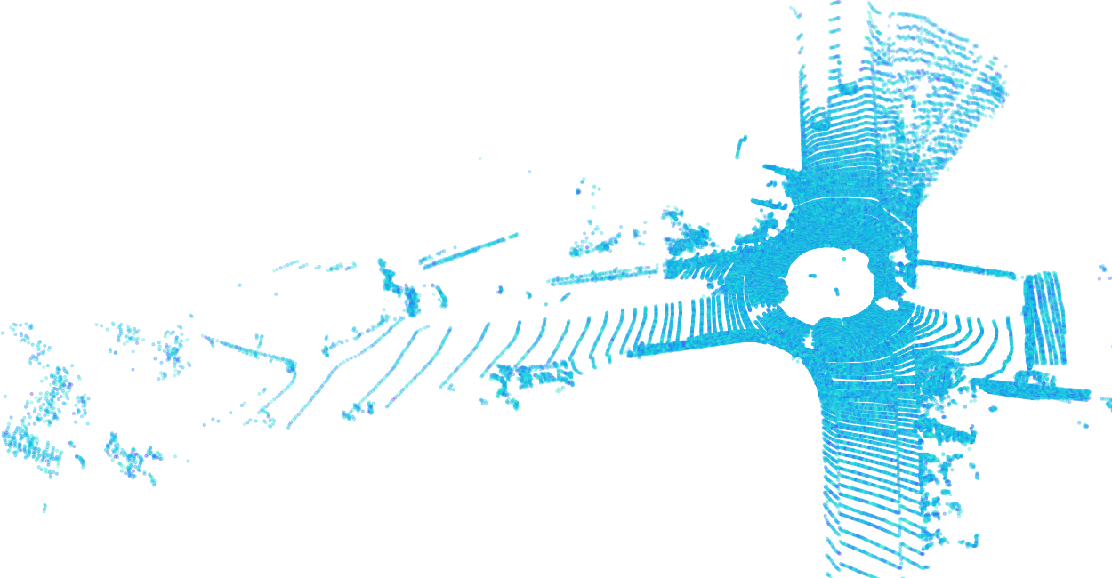
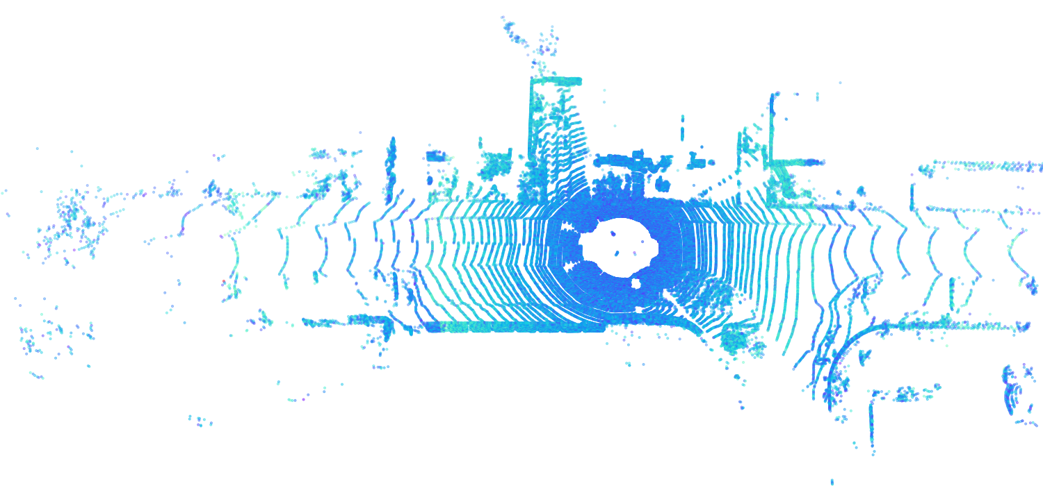
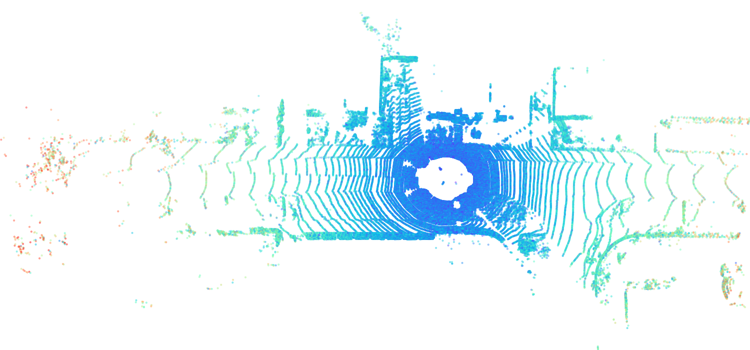
Nevertheless, the aforementioned learned methods overlook a crucial feature of spinning LiDAR point clouds. Fig. 1(a) visualizes a spinning LiDAR point cloud. This LiDAR generates numerous circular-shaped point chains within the point clouds, leading to high redundancy. The predictive geometry in G-PCC utilizes spherical coordinates for encoding point chains, but it solely uses the information of points within the same chain as references, disregarding other neighboring points. The Cylindrical coordinates (Sridhara, Pavez, and Ortega 2021) inadequately represent point clouds since points in the same chain have different coordinates, causing separation in different voxels, as shown in Fig. 1(b)-right. Fortunately, inspired by predictive geometry, we find these points share the same azimuthal angle, leading to the use of Spherical coordinates where the azimuthal angle replaces the coordinate. This transformation allows points in the same chain to be split in the same voxel, concentrating the relevant information, as shown in Fig. 1(c).
In this paper, we focus on the spinning LiDAR point cloud, which is called LiDAR PC for abbreviation. To fully leverage the circular-shaped azimuthal-angle-invariant point chains in LiDAR PCs, we introduce a model-agnostic Spherical-Coordinate-based learned Point cloud compression (SCP) method. SCP transforms LiDAR PCs from Cartesian coordinates to Spherical coordinates, concentrating the relevant information and making it easier for neural networks to reduce redundancy. It’s important to note that, as SCP primarily alters the data pre-processing methods, it is model-agnostic and can be applied to various learned point cloud compression methods. In our experiments, we demonstrate its effectiveness by applying SCP to recent Cartesian-coordinate-based methods like EHEM (Song et al. 2023) and OctAttention (Fu et al. 2022). Additionally, as shown in Fig. 2, the distant voxels in the Spherical-coordinate-based Octree have larger voxel sizes than the central voxels, and the voxel size is positively correlated with the reconstruction errors, resulting in higher reconstruction errors for distant voxels. To solve this problem, we propose a multi-level Octree for SCP, which assigns additional levels to distant voxels. With more levels, the voxel size decreases, leading to lower reconstruction errors.
We trained and evaluated the baseline methods and SCP on the SemanticKITTI (Behley et al. 2019) and Ford (Pandey, McBride, and Eustice 2011) datasets. According to our experiment results, SCP surpasses previous state-of-the-art methods in all conducted experiments. The contributions of our work can be summarized as follows:
-
•
We introduce a model-agnostic Spherical-Coordinate-based learned Point cloud compression (SCP) method. This method transforms point clouds into Spherical coordinates, thereby fully leveraging the circular shapes and the azimuthal angle invariance feature inherent in LiDAR PCs.
-
•
We propose a multi-level Octree structure, which mitigates the increment of reconstruction error of distant voxels in the Spherical-coordinate-based Octree.
-
•
Our experiments on various backbone methods demonstrate that our methods can efficiently reduce redundancy among points, surpassing previous state-of-the-art methods by up to 29.14% in point-to-point PSNR BD-Rate (Bruylants, Munteanu, and Schelkens 2015).
Related Work
Hand-Crafted Methods
Hand-crafted methods based on geometry typically employ tree structures like Octree (Jackins and Tanimoto 1980; Garcia and de Queiroz 2018; Unno et al. 2023) and predictive geometry (ISO/IEC JTC 1/SC 29/WC 7 2019) to organize unstructured point clouds. The Octree structure is widely used in numerous methods, such as (Huang et al. 2008; Kammerl et al. 2012). Predictive geometry, on the other hand, models LiDAR PCs as a predictive tree, where each branch represents a complete point chain scanned by a laser beam. This approach leverages the circular chain structure in LiDAR PCs to predict subsequent points based on the angles and distances of previous points in the chain. Leveraging the circular shape of LiDAR PCs, (Sridhara, Pavez, and Ortega 2021) proposed a transformation from Cartesian-coordinate-based positions to Cylindrical coordinates. This approach, being sensitive to circular shapes, enhances the performance of the G-PCC algorithm in compressing point clouds.
Learned Point Cloud Compression Methods
In recent years, learned point cloud compression methods have been emerging. Many of these techniques, including those cited in (Nguyen et al. 2021b; Quach, Valenzise, and Dufaux 2019; Que, Lu, and Xu 2021; Nguyen et al. 2021a; Wang et al. 2022), utilize Octree to represent and compress point clouds.
OctSqueeze (Huang et al. 2020) builds the Octree of the point cloud, predicting voxel occupancy level by level, using information from ancient voxels and known data about the current voxel. Building upon OctSqueeze, methods such as VoxelDNN (Nguyen et al. 2021a), VoxelContext-Net (Que, Lu, and Xu 2021), SparsePCGC (Wang et al. 2022), and OctFormer (Cui et al. 2023) eliminate redundancy by employing the information of neighbor voxels of the parent voxel. Moreover, Surface Prior (Chen et al. 2022) incorporates neighbor voxels which share the same depth as the current coding voxel, into the framework. OctAttention (Fu et al. 2022) further utilizes this kind of voxel, increasing the context size from surrounding 26 voxels to 1024 voxels. This significantly expands the receptive field of the current voxel. Building on OctAttention, EHEM (Song et al. 2023) further exploits the potential of the Transformer framework by integrating the Swin Transformer (Liu et al. 2021) into their method. This effectively increases the context size to 8192 sibling voxels. Simultaneously, it transitions from serial coding to a checkerboard (He et al. 2021a) type, resulting in a substantial reduction in decoding time. In another aspect, (Chen et al. 2022) employs a context with uncle voxels and utilizes the feature of circular shapes in the LiDAR PCs by incorporating a geometry-prior loss for training.
Preliminary
In this section, we explain the Octree structure, which efficiently represents the point clouds. Then the coordinate systems involved in our proposed method are introduced. Finally, our optimizing target is illustrated.
Octree Structure
The Octree is a hierarchical data structure that provides an efficient way of representing 3D point clouds and is beneficial for dealing with inherently unstructured and sparse LiDAR PCs. When constructing the Octree, the whole point cloud is taken as a cube, a.k.a a voxel, then divided into 8 equal-sized sub-voxels. This procedure repeats until the side length of a leaf voxel is equal to the quantization step. Then the quantization operation merges points in the same leaf voxel together. In each non-leaf voxel, the sub-voxels with points in them are represented by a bit , and the empty ones are set to value . Therefore, each non-leaf voxel is represented by an occupancy symbol composed of 8 bits , where each bit indicates the occupancy status of the corresponding sub-voxel.
Coordinate Systems
We introduce different coordinate systems involved in our experiments: 3-D Cartesian coordinates, Cylindrical coordinates, and Spherical coordinates.
3-D Cartesian Coordinate System
describes each point in the space by 3 numerical coordinates, which are the signed distances from the point to three mutually perpendicular planes. These coordinates are given as .
Cylindrical Coordinate System
is a natural extension of polar coordinates. It describes a point by three values: radial distance from the origin, the angular coordinate (the same as in polar coordinates), and the height , which is the same as in Cartesian coordinates. The transformation from Cartesian coordinates to Cylindrical coordinates can be written as:
| (1) |
note that the quadrant of is decided by signs of and .
Spherical Coordinate System
also describes a point with three values: the radial distance from the origin to the point, and two angles: the polar angle , which is the same angle used in cylindrical coordinates, and the azimuthal angle , which is the angle from the positive coordinate to the point. The transformation equations from Cartesian coordinates are:
| (2) |
again, the quadrant of depends on the signs of and .
Task Definition
The occupancy sequence ( is the number of voxels) of voxels in an Octree is losslessly encoded by an entropy encoder into a bitstream, based on the predicted probability from a neural network. After transmission, the Octree is reconstructed from the entropy-decoded occupancy sequence and converted back into the point cloud. Hence, the objective of point cloud geometry compression is to predict the occupancy of each voxel in the Octree, which can be viewed as a 255-category classification problem. Given all the parameters in our model as and context information as , the optimization objective is the cross-entropy between the ground truth occupancy value and the corresponding predicted probability of each voxel . This can be defined as follows:
| (3) |
Methodology
We propose a model-agnostic Spherical-Coordinate-based learned Point cloud compression (SCP) method, which efficiently leverages the features of LiDAR PCs. Furthermore, we introduce a multi-level Octree method to solve the higher reconstruction errors problem for distant voxels in the Spherical-coordinate-based Octree.
Spherical-Coordinate-based Learned Point Cloud Compression
The circular shapes and azimuthal angle invariance features in LiDAR PCs lead to a high degree of redundancy. In common-used Cartesian coordinates, redundant points are segmented into discrete voxels, as shown in Fig. 1(a). This segmentation creates an unstable context, in which nearby voxels may not be relevant.
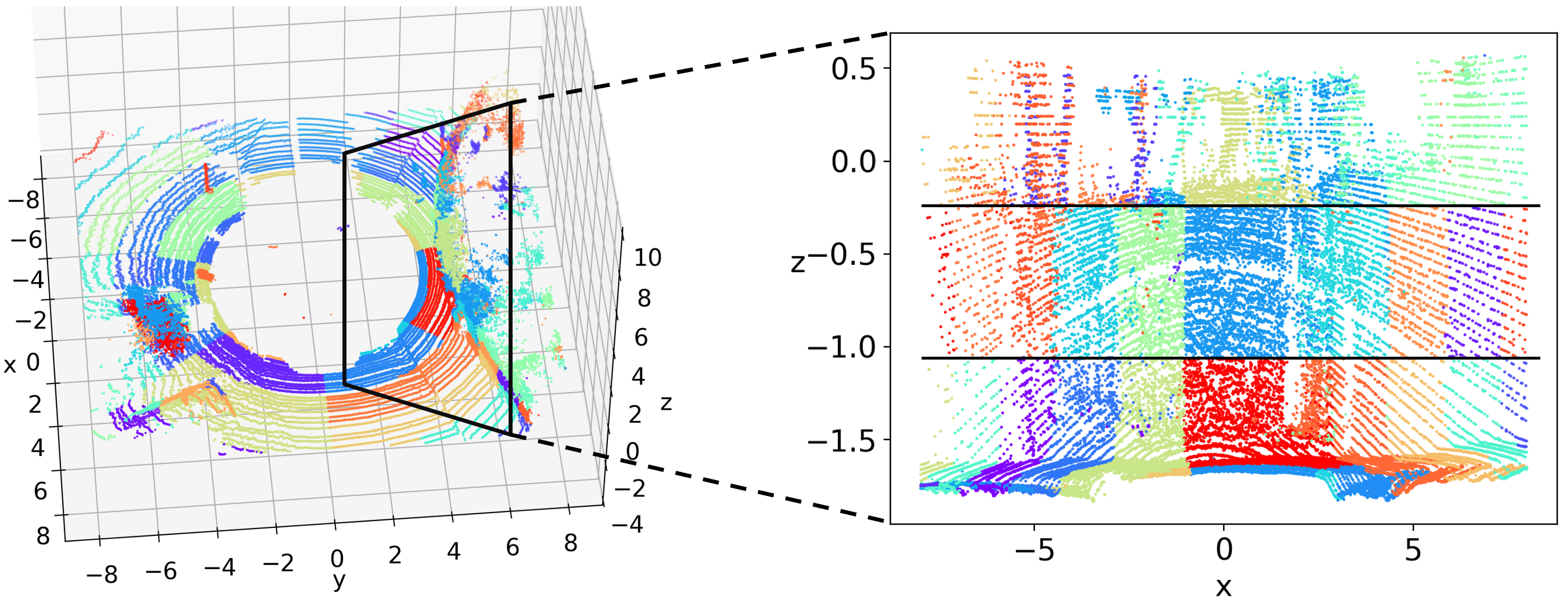
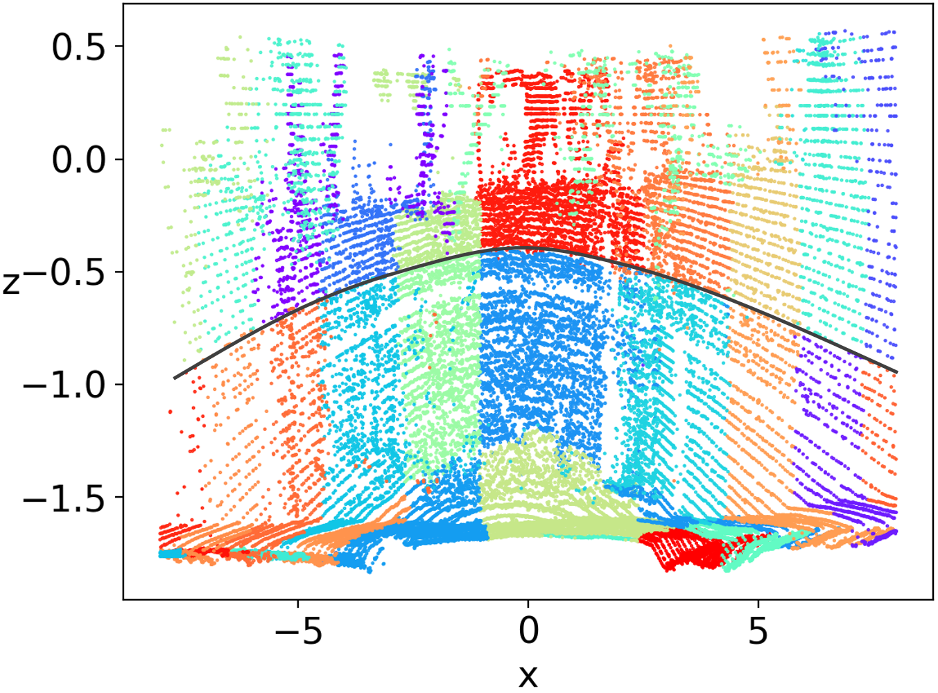
To leverage both features of LiDAR PCs, we propose the Spherical-Coordinate-based learned Point cloud Compression (SCP) method, which converts the points from Cartesian coordinates to Spherical coordinates. When looking up-down, the Spherical-coordinate-based Octree has the same structure as the Cylindrical one, as shown in Fig. 1(a)-left. Points in the same chain are assigned together, making better usage of circular shapes. On the other hand, when looking horizontally from the original point, the Spherical-coordinate-based Octree (Fig. 1(c)) is more likely to assign the points in the same chain to the same voxel compared with the Cylindrical one (Fig. 1(a)-right), harnessing the azimuthal angle invariance feature. Furthermore, the representation of circular structures in Spherical coordinates is simplified from quadratic to linear, making the prediction problem easier to solve, as illustrated in Fig. 3.
When constructing Octree in Spherical coordinates, the quantization procedure differs from that in Cartesian coordinates. The variation range for the , and coordinates in Spherical coordinates are , and , respectively. The varies in different point clouds. When quantizing the point clouds, we adopt the quantization step of EHEM (Song et al. 2023) to the coordinate, noted as . Therefore, the total number of bins for coordinate is . Subsequently, we divide the ranges of the and coordinates by separately to generate their respective quantization steps, as demonstrated in Eq.(LABEL:eq:qs).
| (4) | ||||
where is the quantization step. By setting these and , the bin number of each coordinate are the same.
Multi-Level Octree for SCP
In the Spherical-coordinate-based Octree, the distance is positively related to the reconstruction error, causing the higher reconstruction error of distant voxels. To maintain a reconstruction error lower or similar to that in Cartesian coordinates, we propose a multi-level Octree for SCP, which allocates additional levels to distant voxels. We initially discuss the relation between distant voxels and reconstruction errors of the quantized point cloud in Cartesian and Spherical coordinates, then illustrate our multi-level Octree method.
For Cartesian coordinates, the upper bound of the error can be expressed as follows:
| (5) |
where represents the original position of point , and is its position after quantization, is the quantization step size. It is obvious that this error is uniformly distributed throughout the entire space of Cartesian coordinates because the upper bound is only related to the quantization step. The complete derivation can be found in the Appendix.
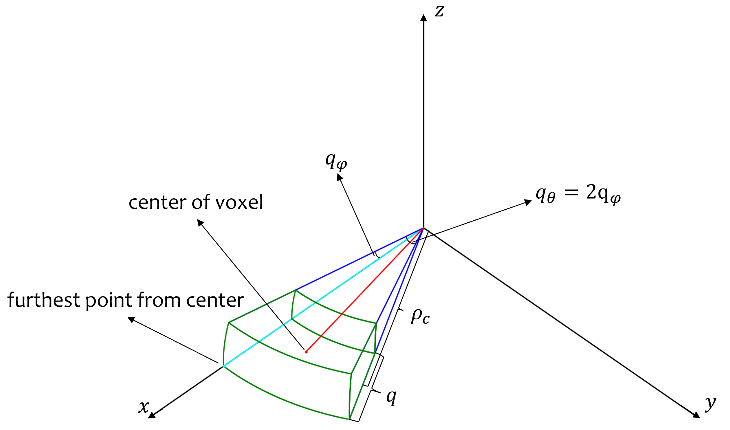
In the Spherical coordinate system, however, the voxels’ reconstruction error is non-uniform. As depicted in Fig. 2, the further a voxel (with a larger value) is from the origin, the larger its size. This characteristic leads to a higher upper bound of reconstruction error for distant voxels. As shown in Eq.(6), the reconstruction error linearly correlated with the value of the coordinate.
| (6) |
We put the proof into the Appendix and further discuss the quantization results in the Experimental Results of the Experiments section.
Based on the above findings, if we allocate additional levels (depths) to the distant areas in the Octree, each added level will reduce the quantization step size of the distant area from to , which in turn halves according to Eq.(6). Motivated by this, we propose a multi-level Octree method to reduce the reconstruction error of distant voxels by adding additional levels. Specifically, we divide the point cloud into parts to assign different numbers of additional levels. Each part has additional levels with , where , , . The assigned extra levels can be represented by the reduction of the quantization , making the reconstruction error upper bound of each part lower or similar to the upper bound of , which can be expressed as
| (7) |
where we assign additional levels for the part . In our experiments, we describe how to pick the optimal for each part to keep .
Experiments
Experiment Settings
Datasets
We compare all the baseline models and SCP on two LiDAR PC datasets, SemanticKITTI (Behley et al. 2019) and Ford (Pandey, McBride, and Eustice 2011). SemanticKITTI comprises 43,552 LiDAR scans obtained from 22 point cloud sequences. The default split for training includes sequences 00 to 10, while sequences 11 to 21 are used for evaluation. We quantize them with a quantization step of with Octree depth . The Ford dataset, utilized in the MPEG point cloud compression standardization, includes three sequences, each containing 1,500 scans. We adhere to the partitioning of the MPEG standardization, where sequence 01 is used for training and sequences 02 and 03 for evaluation. Each sequence in the Ford dataset contains an average of 100,000 points per frame and is quantized to a precision of 1mm. We set the quantization step to with Octree depth . Both settings are the same as EHEM.
Metrics

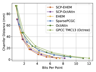
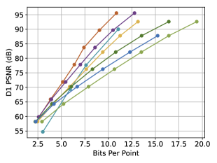
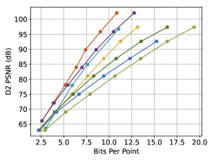
We evaluate point cloud compression methods across two dimensions: rate and distortion. The rate is measured in bits per point (bpp), which is the quotient of the bitstream length and the number of points. For distortion, we employ the most frequently used three metrics: point-to-point PSNR (D1 PSNR), point-to-plane PSNR (D2 PSNR) (ISO/IEC JTC 1/SC 29/WG 7 2021), and Chamfer distance (CD). These metrics are adopted in the former methods, such as EHEM (Song et al. 2023) and OctAttention (Fu et al. 2022), making them convenient to compare with former methods. We also employ BD-Rate (Bruylants, Munteanu, and Schelkens 2015) to illustrate our experimental results clearly. Following EHEM (Song et al. 2023) and (Biswas et al. 2020), we set the peak value of PSNR to 59.70 for SemanticKITTI and 30000 for Ford.
Implementation Details
Our experiments are conducted on OctAttention (Fu et al. 2022) and our reproduced EHEM (Song et al. 2023), as the official implementation of EHEM is not provided. During training, we input the information of Spherical-coordinate-based Octree to the models, including the following information: (1) Octant: the integer order of the current voxel in the parent voxel, in the range of ; (2) Level: the integer depth of the current voxel in the Octree, in the range of and for SemanticKITTI and Ford, respectively; (3) Occupancy, Octant, Level of ancient voxels: All the information of former levels. We trace back 3 levels, the same as OctAttention (Fu et al. 2022); (4) Position: three floating-point positions of the current voxel in the Spherical coordinates, regularized to range .
For the multi-level Octree method, we can deduce from Eq.(5) and Eq.(6) that at approximately , respectively. On the other hand, SCP predicts the distribution of each part separately, which means we repeat the processing of the first several levels times. Hence, for efficiency, is set to the inverse of the power of 2, which utmost reduces repetition. In our experiments, to keep the reconstruction error of SCP lower than that in Cartesian coordinates, we set and , which divides the point clouds into 3 parts: the inner part with , the middle part with , and outer part with . This splitting method constrains the upper bound of the reconstruction error to be lower or equal to the one in Cartesian coordinates for most areas, thereby achieving similar or better reconstruction results for both distant and central parts in LiDAR PCs.
We train SCP models on SemanticKITTI and Ford datasets for 20 and 150 epochs, respectively. We employ the default Adam optimizer (Kingma and Ba 2014) for all experiments with a learning rate of . All the experiments are done on a server with 8 NVIDIA A100 GPUs and 2 AMD EPYC 7742 64-core CPUs.
Baselines
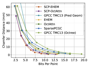
We use recent methods as our baseline to verify the effectiveness of our SCP method. These methods include the state-of-the-art EHEM (Song et al. 2023), which employs the Swin Transformer (Liu et al. 2021) and checkerboard (He et al. 2021a) to compress point clouds; the sparse-CNN-based method SparsePCGC (Wang et al. 2022), which achieves high compression performance with an end-to-end scheme; the aforementioned OctAttention (Fu et al. 2022), which uses the Transformer and sibling voxel contexts; and the MPEG G-PCC TMC13 (ISO/IEC JTC 1/SC 29/WC 7 2021) with either Octree or predictive geometry, which is the mainstream hand-crafted compression method. Note that the predictive geometry is only available for the Ford dataset since the SemanticKITTI dataset lacks the necessary sensor information for the calculation of predictive geometry.
| Method | Depth=12 | Depth=14 | Depth=16 |
| G-PCC | 0.22 / 0.06 | 0.63 / 0.21 | 1.05 / 0.39 |
| EHEM | 0.60 / 0.57 | 1.48 / 1.57 | 2.92 / 3.13 |
| SCP-E w/o | 0.63 / 0.62 | 1.73 / 1.86 | 3.21 / 3.49 |
| SCP-EHEM | 1.16 / 1.11 | 2.34 / 2.41 | 3.92 / 4.09 |
Experimental Results
We designate SCP with a multi-level Octree as the default method, referred to as “SCP”, while the SCP method without a multi-level Octree is called “SCP w/o multi-level” or “SCP w/o”. The SCP methods with EHEM (Song et al. 2023) and OctAttention (Fu et al. 2022) as the backbone are represented as “SCP-EHEM” and “SCP-OctAttn”, respectively.
Quantitative results
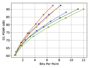
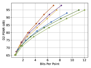
As depicted in Fig. 4, our SCP-EHEM models achieve significant improvement when compared with all the baselines. SCP achieves a 61.23% D1 PSNR BD-Rate gain on the SemanticKITTI dataset and 72.54% on the Ford dataset when compared with Octree-based G-PCC. On the other hand, SCP-EHEM and SCP-OctAttention models outperform the baseline methods by 13.02% and 29.14% D1 PSNR BD-rate improvement on the SemanticKITTI dataset, respectively; 25.54% and 24.78% on the Ford dataset, respectively. Remarkably, SCP-OctAttention even surpasses the original EHEM method, which has an 8 times larger receptive field than OctAttention. Our results on D2 PSNR and CD metrics also significantly outperform the previous method, demonstrating the robustness of SCP in efficiently compressing various point clouds under different driving environments for point cloud acquisition. For the results of predictive-geometry-based G-PCC on the Ford dataset, it has a much better performance than the Octree-based one except for the lowest reconstruction quality. However, it is surpassed by both SCP-EHEM and SCP-OctAttention because of the lack of context information. All these experiments showcase the universality of our SCP, which can be applied to various learned methods to fully leverage the circular feature of LiDAR PCs and improve the performance of these methods.
We show the inference time comparisons among G-PCC, the reproduced EHEM, SCP-EHEM without multi-level Octree (SCP-E w/o), and SCP-EHEM in Table 1. The reconstruction performance of SCP-E w/o is better than the original Cartesian-coordinate-based EHEM because Spherical-coordinate-based Octree has lower reconstruction error in the central parts, which contain most points in the point cloud. This reserves more individual points after quantization, leading to a correspondingly longer processing time. On the other hand, one limitation of SCP-EHEM is that it repeats calculations of the beginning levels for each part, resulting in time overhead, which can be eliminated by processing the former levels together for all 3 parts. We will solve the problem of this overhead in our future work.
Qualitative results
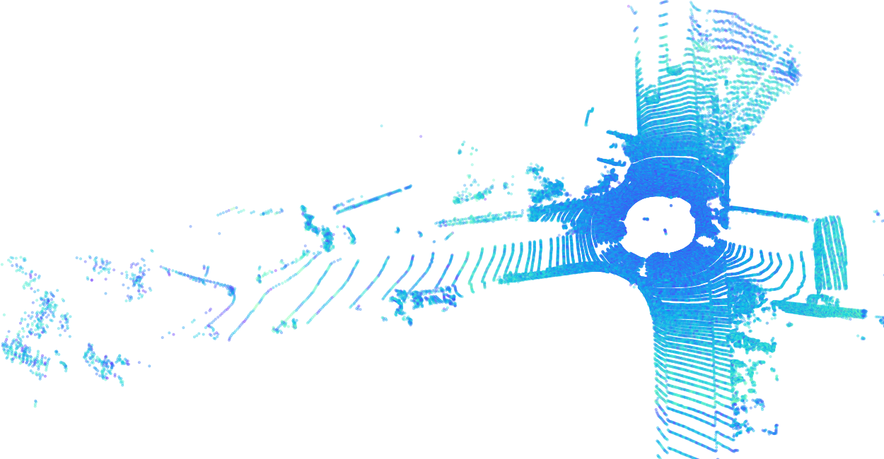
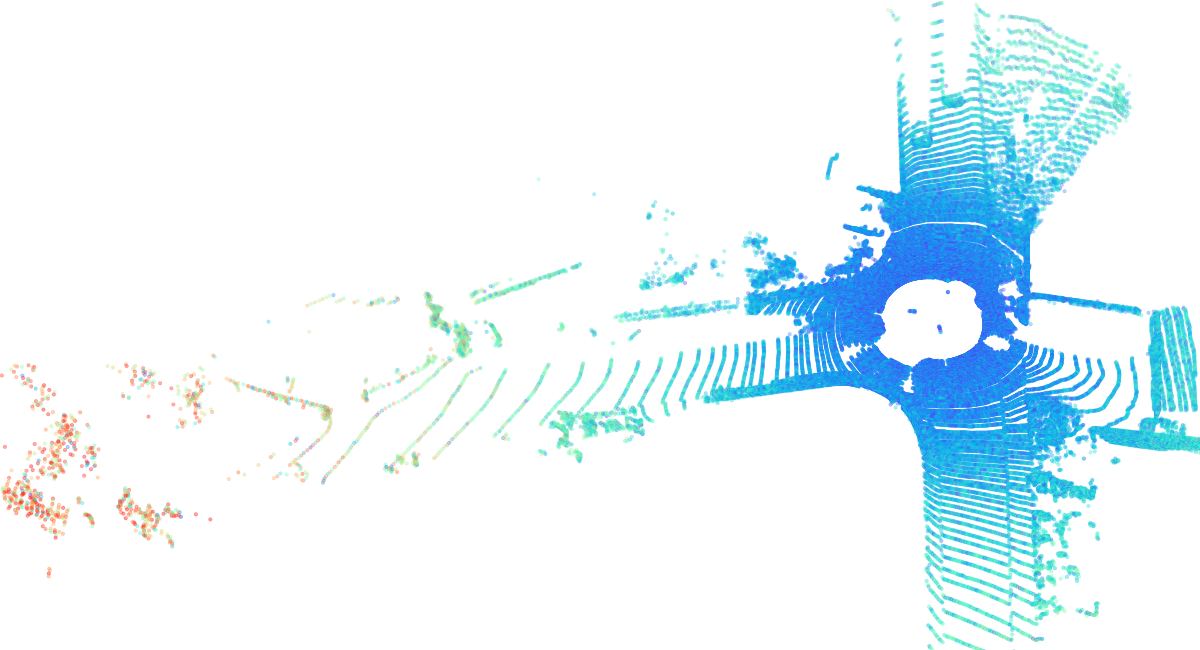
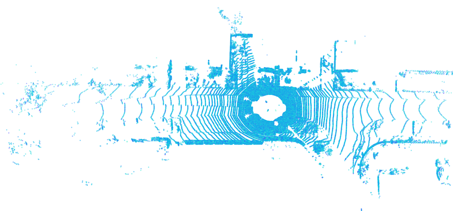
As depicted in Fig. 5, we visualize the reconstruction errors for point clouds in the SemanticKITTI dataset. The errors are represented with a rainbow color scheme, where purple indicates lower error and red signifies higher error. It is evident that the central parts of Fig. 5(b) and Fig. 5(e) have lower errors than those of Fig. 5(a) and Fig. 5(d), while the distant parts of our method exhibit similar reconstruction errors. In another perspective, the distant area of Fig. 5(c) and Fig. 5(f) exhibit significantly higher errors compared to the central areas. This issue is substantially mitigated following the application of our multi-level Octree method, as demonstrated in Fig. 5(b) and Fig. 5(e).
Ablation Study
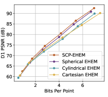
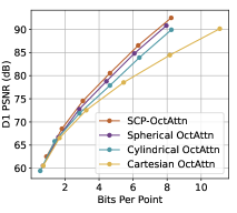
To validate the effectiveness of SCP and the multi-level Octree method, we conducted ablation studies on them, as shown in Fig. 6. For the selection of metric, we find the curve tendencies of 3 metrics in Fig. 4 are similar, so we follow the ablation settings of EHEM, using D1 PSNR as the metric.
To verify the good performance of SCP, we experiment on all three coordinate systems, Spherical, Cylindrical, and Cartesian, with both backbone models EHEM and OctAttention. Note that the Cartesian-coordinate-based methods are the original EHEM/OctAttention. These experiments are conducted without the multi-level Octree method because it is designed for angle-based coordinate systems and is not applicable to Cartesian-coordinate-based Octree. As shown in Fig. 6, Spherical-coordinate-based methods (Spherical ones) are better than both the Cartesian-coordinate-based ones (Cartesian methods) and the Cylindrical-coordinate-based ones (Cylindrical methods). As mentioned in Fig. 1, the Octree under Spherical coordinates has better relevant context for each point in the point cloud than that under Cylindrical/Cartesian coordinates. The improvement is introduced by the azimuthal coordinate and polar (, ) coordinates in the Spherical coordinate system. For the ablation study on the multi-level Octree method, our SCP methods outperform the version without our multi-level Octree method (SCP- w/o), proving the effectiveness of our method.
Conclusion
We introduce a model-agnostic Spherical-Coordinate-based learned Point cloud compression (SCP) method that effectively leverages the circular shapes and azimuthal angle invariance feature present in spinning LiDAR point clouds. Concurrently, we address the higher reconstruction error issue in distant areas of the Spherical-coordinate-based Octree by implementing a multi-level Octree method. Our techniques exhibit high universality, making them applicable to a wide range of learned point cloud compression methods. Experimental results on two backbone methods, EHEM and OctAttention, exhibit the high effectiveness of our SCP and multi-level Octree method. On the other hand, our methods still have the potential to be improved on the inference time, which will be done in our future work.
Acknowledgments
These research results were obtained from the commissioned research (No. JPJ012368C06801, JPJ012368C03801) by National Institute of Information and Communications Technology (NICT), Japan; JSPS KAKENHI Grant Number JP23K16861.
References
- Behley et al. (2019) Behley, J.; Garbade, M.; Milioto, A.; Quenzel, J.; Behnke, S.; Stachniss, C.; and Gall, J. 2019. Semantickitti: A dataset for semantic scene understanding of lidar sequences. In Proceedings of the IEEE/CVF international conference on computer vision, 9297–9307.
- Biswas et al. (2020) Biswas, S.; Liu, J.; Wong, K.; Wang, S.; and Urtasun, R. 2020. Muscle: Multi sweep compression of lidar using deep entropy models. Advances in Neural Information Processing Systems, 33: 22170–22181.
- Bruylants, Munteanu, and Schelkens (2015) Bruylants, T.; Munteanu, A.; and Schelkens, P. 2015. Wavelet based volumetric medical image compression. Signal processing: Image communication, 31: 112–133.
- Chen et al. (2022) Chen, Z.; Qian, Z.; Wang, S.; and Chen, Q. 2022. Point Cloud Compression with Sibling Context and Surface Priors. In European Conference on Computer Vision, 744–759. Springer.
- Choe et al. (2021) Choe, J.; Joung, B.; Rameau, F.; Park, J.; and Kweon, I. S. 2021. Deep point cloud reconstruction. arXiv preprint arXiv:2111.11704.
- Cui et al. (2023) Cui, M.; Long, J.; Feng, M.; Li, B.; and Kai, H. 2023. OctFormer: Efficient Octree-Based Transformer for Point Cloud Compression with Local Enhancement. In Proceedings of the AAAI Conference on Artificial Intelligence, volume 37, 470–478.
- Fernandes et al. (2021) Fernandes, D.; Silva, A.; Névoa, R.; Simões, C.; Gonzalez, D.; Guevara, M.; Novais, P.; Monteiro, J.; and Melo-Pinto, P. 2021. Point-cloud based 3D object detection and classification methods for self-driving applications: A survey and taxonomy. Information Fusion, 68: 161–191.
- Fu et al. (2022) Fu, C.; Li, G.; Song, R.; Gao, W.; and Liu, S. 2022. Octattention: Octree-based large-scale contexts model for point cloud compression. In Proceedings of the AAAI Conference on Artificial Intelligence, volume 36, 625–633.
- Garcia and de Queiroz (2018) Garcia, D. C.; and de Queiroz, R. L. 2018. Intra-frame context-based octree coding for point-cloud geometry. In 2018 25th IEEE International Conference on Image Processing (ICIP), 1807–1811. IEEE.
- He et al. (2021a) He, D.; Zheng, Y.; Sun, B.; Wang, Y.; and Qin, H. 2021a. Checkerboard context model for efficient learned image compression. In Proceedings of the IEEE/CVF Conference on Computer Vision and Pattern Recognition, 14771–14780.
- He et al. (2021b) He, Y.; Huang, H.; Fan, H.; Chen, Q.; and Sun, J. 2021b. Ffb6d: A full flow bidirectional fusion network for 6d pose estimation. In Proceedings of the IEEE/CVF Conference on Computer Vision and Pattern Recognition, 3003–3013.
- He et al. (2020) He, Y.; Sun, W.; Huang, H.; Liu, J.; Fan, H.; and Sun, J. 2020. Pvn3d: A deep point-wise 3d keypoints voting network for 6dof pose estimation. In Proceedings of the IEEE/CVF conference on computer vision and pattern recognition, 11632–11641.
- Huang et al. (2020) Huang, L.; Wang, S.; Wong, K.; Liu, J.; and Urtasun, R. 2020. Octsqueeze: Octree-structured entropy model for lidar compression. In Proceedings of the IEEE/CVF conference on computer vision and pattern recognition, 1313–1323.
- Huang et al. (2008) Huang, Y.; Peng, J.; Kuo, C.-C. J.; and Gopi, M. 2008. A generic scheme for progressive point cloud coding. IEEE Transactions on Visualization and Computer Graphics, 14(2): 440–453.
- ISO/IEC JTC 1/SC 29/WC 7 (2019) ISO/IEC JTC 1/SC 29/WC 7. 2019. Predictive Geometry Coding. M51012.
- ISO/IEC JTC 1/SC 29/WC 7 (2021) ISO/IEC JTC 1/SC 29/WC 7. 2021. Mpeg g-pcc tmc13. https://github.com/MPEGGroup/mpeg-pcc-tmc13.
- ISO/IEC JTC 1/SC 29/WG 7 (2021) ISO/IEC JTC 1/SC 29/WG 7. 2021. Common test conditions for g-pcc. N00106.
- Jackins and Tanimoto (1980) Jackins, C. L.; and Tanimoto, S. L. 1980. Oct-trees and their use in representing three-dimensional objects. Computer Graphics and Image Processing, 14(3): 249–270.
- Kammerl et al. (2012) Kammerl, J.; Blodow, N.; Rusu, R. B.; Gedikli, S.; Beetz, M.; and Steinbach, E. 2012. Real-time compression of point cloud streams. In 2012 IEEE international conference on robotics and automation, 778–785. IEEE.
- Kingma and Ba (2014) Kingma, D. P.; and Ba, J. 2014. Adam: A method for stochastic optimization. arXiv preprint arXiv:1412.6980.
- Li et al. (2021) Li, R.; Li, X.; Heng, P.-A.; and Fu, C.-W. 2021. Point cloud upsampling via disentangled refinement. In Proceedings of the IEEE/CVF conference on computer vision and pattern recognition, 344–353.
- Li et al. (2020) Li, Y.; Ma, L.; Zhong, Z.; Liu, F.; Chapman, M. A.; Cao, D.; and Li, J. 2020. Deep learning for lidar point clouds in autonomous driving: A review. IEEE Transactions on Neural Networks and Learning Systems, 32(8): 3412–3432.
- Liu et al. (2021) Liu, Z.; Lin, Y.; Cao, Y.; Hu, H.; Wei, Y.; Zhang, Z.; Lin, S.; and Guo, B. 2021. Swin transformer: Hierarchical vision transformer using shifted windows. In Proceedings of the IEEE/CVF international conference on computer vision, 10012–10022.
- Nguyen et al. (2021a) Nguyen, D. T.; Quach, M.; Valenzise, G.; and Duhamel, P. 2021a. Learning-based lossless compression of 3d point cloud geometry. In ICASSP 2021-2021 IEEE International Conference on Acoustics, Speech and Signal Processing (ICASSP), 4220–4224. IEEE.
- Nguyen et al. (2021b) Nguyen, D. T.; Quach, M.; Valenzise, G.; and Duhamel, P. 2021b. Learning-based lossless compression of 3d point cloud geometry. In ICASSP 2021-2021 IEEE International Conference on Acoustics, Speech and Signal Processing (ICASSP), 4220–4224. IEEE.
- Pandey, McBride, and Eustice (2011) Pandey, G.; McBride, J. R.; and Eustice, R. M. 2011. Ford campus vision and lidar data set. The International Journal of Robotics Research, 30(13): 1543–1552.
- Quach, Valenzise, and Dufaux (2019) Quach, M.; Valenzise, G.; and Dufaux, F. 2019. Learning convolutional transforms for lossy point cloud geometry compression. In 2019 IEEE international conference on image processing (ICIP), 4320–4324. IEEE.
- Que, Lu, and Xu (2021) Que, Z.; Lu, G.; and Xu, D. 2021. Voxelcontext-net: An octree based framework for point cloud compression. In Proceedings of the IEEE/CVF Conference on Computer Vision and Pattern Recognition, 6042–6051.
- Silva et al. (2023) Silva, A. L.; Oliveira, P.; Durães, D.; Fernandes, D.; Névoa, R.; Monteiro, J.; Melo-Pinto, P.; Machado, J.; and Novais, P. 2023. A Framework for Representing, Building and Reusing Novel State-of-the-Art Three-Dimensional Object Detection Models in Point Clouds Targeting Self-Driving Applications. Sensors, 23(14): 6427.
- Song et al. (2023) Song, R.; Fu, C.; Liu, S.; and Li, G. 2023. Efficient Hierarchical Entropy Model for Learned Point Cloud Compression. In Proceedings of the IEEE/CVF Conference on Computer Vision and Pattern Recognition (CVPR), 14368–14377.
- Sridhara, Pavez, and Ortega (2021) Sridhara, S. N.; Pavez, E.; and Ortega, A. 2021. Cylindrical coordinates for LiDAR point cloud compression. In 2021 IEEE International Conference on Image Processing (ICIP), 3083–3087. IEEE.
- Unno et al. (2023) Unno, K.; Matsuzaki, K.; Komorita, S.; and Kawamura, K. 2023. Rate-Distortion Optimized Variable-Node-size Trisoup for Point Cloud Coding. In ICASSP 2023-2023 IEEE International Conference on Acoustics, Speech and Signal Processing (ICASSP), 1–5. IEEE.
- Wang et al. (2019) Wang, C.; Xu, D.; Zhu, Y.; Martín-Martín, R.; Lu, C.; Fei-Fei, L.; and Savarese, S. 2019. Densefusion: 6d object pose estimation by iterative dense fusion. In Proceedings of the IEEE/CVF conference on computer vision and pattern recognition, 3343–3352.
- Wang et al. (2022) Wang, J.; Ding, D.; Li, Z.; Feng, X.; Cao, C.; and Ma, Z. 2022. Sparse tensor-based multiscale representation for point cloud geometry compression. IEEE Transactions on Pattern Analysis and Machine Intelligence.
- Zhu et al. (2021) Zhu, X.; Zhou, H.; Wang, T.; Hong, F.; Ma, Y.; Li, W.; Li, H.; and Lin, D. 2021. Cylindrical and asymmetrical 3d convolution networks for lidar segmentation. In CVPR, 9939–9948.
Appendix
Reconstruction error of Cartesian coordinates and Spherical coordinates
We illustrate the derivation of Eq.(5) and Eq.(6) in this section. We use the -norm to evaluate the reconstruction error. This -norm is used in all three metrics in our experiments.
For the Octree in Cartesian coordinates, the leaf voxels are cubes whose side length is quantization step . The position of a voxel is the center of it, marked as . The upper bound of reconstruction error can be reached at the corners of the cube, one of which can be written as . Therefore, the upper bound of reconstruction error in Cartesian coordinates is
| (8) |
To compare with former methods, we need to convert Spherical coordinates back to Cartesian coordinates for reconstruction error calculation. In Spherical coordinates, the size of voxels is only relevant to coordinate , therefore, we analyze the one voxel beside coordinate , as the green box shown in Fig. 7, which is easier for derivation. The voxel center can be marked as . We use to replace according to Eq.(LABEL:eq:qs). In the most situation, is much smaller that , so we can set , . Then the position can be rewritten as: . On the other hand, one of the furthest points in the voxel is indicated in Fig. 7. The position of it is , which can be approximated as since is much smaller than . In conclusion, the upper bound of the reconstruction error can be derived by calculating the distance between these two points, as shown in Eq.(9).
| (9) |