Search for continuous gravitational waves from neutron stars in five globular clusters with a phase-tracking hidden Markov model in the third LIGO observing run
Abstract
A search is performed for continuous gravitational waves emitted by unknown neutron stars in five nearby globular clusters using data from the third Laser Interferometer Gravitational-Wave Observatory (LIGO) observing run, over the frequency range –. The search uses a hidden Markov model to track both the frequency and phase of the continuous wave signal from one coherent segment to the next. It represents the first time that a phase-tracking hidden Markov model has been used in a LIGO search. After applying vetoes to reject candidates consistent with non-Gaussian artifacts, no significant candidates are detected. Estimates of the strain sensitivity at 95% confidence and corresponding neutron star ellipticity are presented. The best strain sensitivity, at , is achieved for the cluster NGC6544.
I Introduction
Continuous gravitational waves (CWs) are long-lasting and nearly monochromatic signals which may be emitted by a variety of sources, but which have so far remained undetected [1, 2]. In the frequency band covered by existing terrestrial interferometers, one promising class of CW sources is rapidly rotating neutron stars located within the Milky Way. There are many possible emission mechanisms through which neutron stars can emit gravitational waves, involving both the crust and the interior. These include deformations created by thermal [3, 4, 5, 6], magnetic [7, 8, 9, 10, 11, 12], and tectonic [13, 14, 15] effects, as well as fluid oscillations (particularly -modes) [16, 17, 18]. CW searches thus serve to probe the physics involved in these mechanisms.
Globular clusters are an interesting target for CW searches, as their dense cores provide a natural formation site for millisecond pulsars (MSPs), fast-spinning neutron stars which have been “recycled” by accretion from a binary companion [19, 20, 21, 22]. The gravitational wave strain scales as the square of the spin frequency for several important emission mechanisms [1]. Once recycled, MSPs may also experience further accretion episodes later in their life, as the stellar density in the cluster core enhances the likelihood of stellar encounters which disrupt the orbits of debris disks [23, 24, 25] or planets around the pulsar [26, 27, 28, 29, 30]. Two CW searches targeting globular clusters specifically have been carried out in the past [2]. Abbott et al. [24] carried out a search with 10 days of Initial Laser Interferometer Gravitational-Wave Observatory (LIGO) Science Run 6 data targeting unknown neutron stars in the globular cluster NGC 6544. Dergachev et al. [31] carried out a search with Advanced LIGO Observing Run 1 data targeting a small sky region containing both the Galactic Center and the globular cluster Terzan 5. Searches directed at the Galactic Center are broadly similar to globular cluster searches, being wide parameter space searches targeting an interesting sky region, and a number of these searches have been performed previously [32, 31, 33, 34]. Besides the two specific searches, globular cluster MSPs have been targeted in searches for known pulsars [35, 36, 37, 38, 39, 34].
This paper presents a search for CW emission from unknown neutron stars in five globular clusters in the Milky Way. We allow for the possibility that the phase model of the signal does not follow a simple Taylor expansion but includes some additional stochasticity (called “spin wandering”). The search uses a hidden Markov model (HMM) to track both the frequency and phase of the wandering signal [40, 41, 42]. HMMs have been used in a number of CW searches in the past [43, 44, 45, 46, 47, 48, 49, 50, 51, 52, 53, 54, 55] but previously tracked only the frequency, typically using the -statistic for isolated targets [56, 57] or the -statistic for targets in binaries [58]. In contrast, the HMM implementation used in this paper, developed by Melatos et al. [42], employs a modified version of the -statistic [59, 42], which is a function of both frequency and phase. Phase tracking improves the sensitivity (by as it turns out) by downweighting noise features, that are not approximately phase-coherent over the search. We opt to use the phase-tracking HMM in this search both to take advantage of its enhanced sensitivity and as a technology demonstration in its own right. This is the first time that a phase-tracking HMM has been used in an astrophysical search, and its successful application here shows that the technique can be feasibly applied to searches over a wide parameter domain.
The structure of the paper is as follows. In Section II we describe the HMM framework in general, its implementation in this specific search, and the modified -statistic which serves as the coherent detection statistic. In Section III we discuss the setup of the search, including target selection and the parameter domain. In Section IV we discuss the candidates returned by the search, the veto procedures used to reject spurious candidates, and the results of applying the vetoes. In Section V we estimate the sensitivity of the search to CW emission from each cluster. In Section VI we summarise the results and look to future work.
II Algorithms
In this section we briefly recap the HMM formalism and its algorithmic components. We define the signal model (Section II.1), derive the form of the phase-sensitive -statistic which serves as the coherent detection statistic throughout this search (Section II.2), and explain how the -statistic is combined with phase-frequency transition probabilities as part of a HMM (Section II.3).
II.1 Signal model
Following Jaranowski et al. [56], the mass quadrupole gravitational wave signal from an isolated rotating neutron star emitting at twice the spin frequency can be written as a linear combination of four components
| (1) |
with , where we adopt the Einstein summation convention. The are the “amplitude parameters” given by Eqs. (32)–(35) in Jaranowski et al. [56]. They do not evolve and depend on the characteristic strain amplitude , the cosine of the inclination angle , the polarisation angle and the initial signal phase .111Strictly speaking the also depend on the angle between the total angular momentum of the star and the axis of symmetry, , as well as the angle between the interferometer arms, [56]. The are multiplied by a factor of , but for the LIGO detectors, and we assume also, so this factor is unity. The are combinations of the antenna pattern functions [Eqs. (12) and (13) of Jaranowski et al. [56]] and the phase of the signal , whose evolution is expanded as a Taylor series, viz.
| (2) |
In Eq. (2), is the -th time derivative of the frequency evaluated at , is an additional stochastic wandering term, the nature of which is discussed in detail in Section II.3.2, and is the phase contribution from the transformation between the solar system barycentre (SSB) and the detector frame, cf. Eq. (14) of Jaranowski et al. [56]. For the form of see Eq. (36) in Ref. [56].
II.2 Phase-dependent -statistic
The -statistic was introduced by Prix and Krishnan [59] as a Bayesian alternative to the well-known -statistic [56]. The -statistic is obtained by analytically maximizing the likelihood function over and hence , , and . The -statistic is obtained by instead marginalising over these parameters with a physically motivated prior which is uniform in , , , and . Melatos et al. [42] modified this approach to leave as a free parameter, so that we can compute the -statistic for many coherent segments and then track and across these segments using a HMM as discussed in Section II.3. Here we briefly justify the form of the phase-dependent -statistic and discuss how to compute it in practice. The discussion draws on Refs. [56, 59, 42].
We begin with the log likelihood
| (3) |
where is the detector data and is the signal as defined in Eqs. (1) and (2). The inner product is defined as
| (4) | ||||
| (5) |
where is the one-sided power spectral density of the noise at a frequency , is the total length of the data, and the approximate equality holds for finite-length signals localized spectrally to a narrow band around in which can be taken as constant (which is a good approximation for the quasi-monochromatic signals of interest here [56]). Defining and we write
| (6) |
The phase-dependent -statistic is obtained by marginalising over , , and :
| (7) |
In Eq. (7), is the prior, where is a large but arbitrary maximum and is an irrelevant normalising constant. Since is a constant and can be taken outside the integral it is dropped going forward.
We now substitute Eq. (6) into Eq. (7) and perform the triple integral. Writing , with independent of , and collapsing the triple integral for notational convenience, we obtain
| (8) |
We use the following identity to perform the integral over :
| (9) |
We also take , which is arbitrary, to be sufficiently large that the second term approaches unity. The result is
| (10) |
The ingredients of the integrand — , and — are all straightforward to compute using existing functionality in lalsuite, the standard software suite for analysis of LIGO, Virgo, and KAGRA data [60]. We use the existing graphics processing unit (GPU) framework [61] to compute the -statistic and hence , the most expensive step. We also integrate Eq. (10) using GPUs, running a simple Simpson integrator on a grid of and values. We verify using synthetic data that the relative error in the value of the -statistic when computed using an grid compared to a finer grid is typically small, with a mean fractional error of 1.9% and a fractional error exceeding 10% occurring in 1.2% of the -statistic values (corresponding to five bands with a coherence time of five days and eight phase bins) computed for the purposes of this test.
II.3 HMMs and the Viterbi algorithm
The number of signal templates needed to cover an astrophysically relevant parameter domain grows quickly for a phase-coherent search, as the observational timespan increases. Hence a number of “semicoherent” techniques for CW searches have been developed, which perform phase-coherent computations on subdivided segments of length and combine the segments without enforcing phase coherence between them. Most semicoherent methods completely discard the phase information between segments (see e.g. Refs. [40, 62, 63, 64]). Some, termed “loosely coherent”, retain some phase information but do not enforce perfect phase continuity [65, 66, 67]. While there is some loss of sensitivity inherent in this approach — the sensitivity of semicoherent searches scales as [62, 68], compared to for coherent searches — there is a large computational saving. Some semicoherent methods also offer flexibility in the face of the unexpected. For example, although fully coherent methods can accommodate deviations away from an assumed signal model through explicit searches over the parameters determining the phase evolution [69, 70, 71], if there is a stochastic component to the phase evolution which operates on timescales shorter than the observing timespan then a semicoherent approach may be needed. A HMM solved by the Viterbi algorithm to find the most likely sequence of signal frequencies is one such approach, which has been used in a number of CW searches in the past [43, 44, 45, 47, 46, 48, 49, 50, 51, 52, 53, 54, 55]. This approach was extended to include tracking of by Melatos et al. [42], and is the subject of the present paper. In this section we review the basic framework of HMMs and the way it is put into practice for the present, loosely coherent search.
II.3.1 HMMs
HMMs model the evolution and observation of systems fulfilling two important criteria: a) the evolution of the internal state of the system is Markovian, and b) the internal state is hidden from the observer but may be probed probabilistically through measurement. This section briefly describes the formalism involved; for a more detailed review of HMMs see Rabiner [72].
The hidden state of the system is assumed here to be discretised and bounded, so that each state is in the set , where is the total number of hidden states. Time is likewise discretised, with the HMM occupying the hidden state at each timestep ,where is an “initial timestep” before any observations have been made. A sequence of possible hidden states occupied during a particular realisation of the HMM is denoted by . The dynamics of the system are captured by the transition matrix , whose entries are defined as
| (11) |
At each timestep we assume that the system is observed. For a given realisation we write the sequence of observations as . The set of possible observations need not be finite, discretised, or bounded. All we require is that there exists an emission probability function defined as
| (12) |
i.e. the probability of observing at the timestep , if the hidden state is occupied at .
Finally we specify a belief about the state of the system at the beginning of the analysis, i.e.
| (13) |
In this paper we have no reason to impose anything other than a uniform prior, viz. .
Given the above ingredients, it is straightforward to compute the probability of a hidden state sequence , given a sequence of observations :
| (14) |
The goal is to compute .
II.3.2 Phase tracking
In this paper, the full observation is divided into segments of length , which are analysed coherently. Each coherent segment is a timestep in the HMM. The hidden states are pairs of frequencies and phases at the start of a segment, . The phase-dependent -statistic, defined in Section II.2, plays the role of . It then remains to specify the transition matrix. We follow Melatos et al. [42] and adopt the following model for the evolution of the signal frequency and phase :
| (15) | ||||
| (16) |
where is a zero-mean white noise term, i.e.
| (17) | ||||
| (18) |
and parametrises the noise strength. The forward transition matrix is readily obtained by solving the Fokker-Planck equation corresponding to Eqs. (15)–(18). For practical reasons it is useful to also know the backward transition matrix
| (19) |
which is similarly obtained by solving the backward Fokker-Planck equation for this system.
Details of the transition matrices are given in Appendix A, and an illustrative figure is shown in Fig. 1.
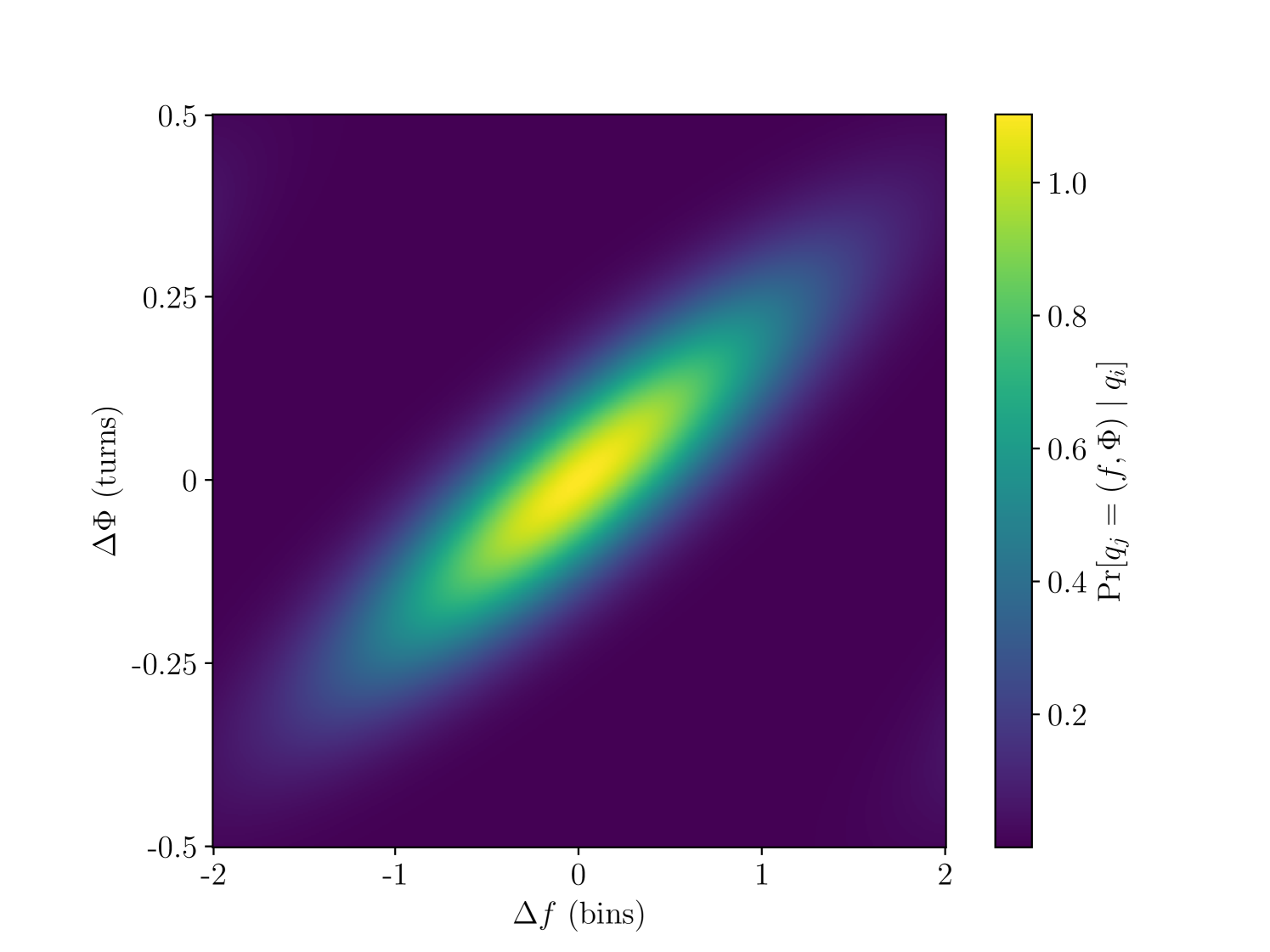
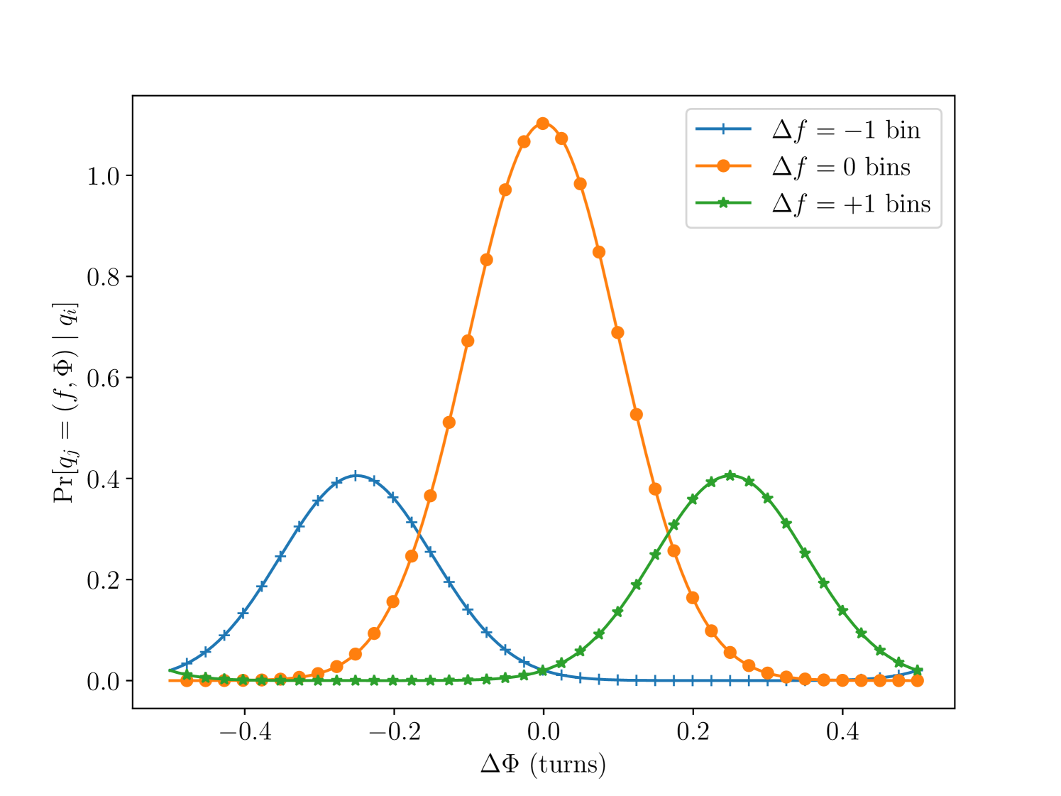
The top panel of Fig. 1 shows a heatmap of as a function of and . As shown in Melatos et al. [42] and Appendix A, it is approximately a truncated Gaussian centred on , with positive covariance between and . The bottom panel shows slices through the distribution at . These slices are the distributions used to compute the transition probabilities in the HMM. The bin distributions are identical up to the location of the peak and each contain approximately 20% of the total probability, while the bin contains the other 60%. The transitions probabilities are broad in phase. All three distributions have similar widths. From this figure we see that the probability is concentrated in the same bin as the previous timestep, but some leakage into neighboring bins does occur.
Melatos et al. [42] included a damping term in Eq. (15). This approximates the tendency of the spin frequency of the neutron star to approach zero in the long term, i.e. it represents the long-term spin down process. In this search we explicitly search over the spin-down rate as a parameter in the deterministic part of the signal model (see Sections III.5.1 and III.6.1), and assume that once the deterministic spin down is taken into account, the mean drift of the signal frequency is negligible. As such, we impose the condition which implies [42]. This renders the effect of in Eq. (15) negligible, and in this work we do not include it. The approximation is justified in more detail in Appendix A.
II.3.3 Optimal Viterbi path
With the HMM fully specified, we turn to the question of to use it in a CW search. To find signal candidates we use the Viterbi algorithm [72, 40] to find the most likely sequence of hidden states,
| (20) |
More precisely, for each possible terminating frequency bin we find the most likely sequence of hidden states which terminates in that bin,
| (21) |
These paths are sorted according to their probability . Paths exceeding a predetermined threshold are marked for follow-up analysis. The determination of the threshold as a function of the desired false alarm probability is discussed in Section IV.1. To maximize numerical accuracy, we work with log probabilities so that the products in Eq. (14) become sums. Hence we threshold candidates according to their log likelihood .
To maximize computational performance the HMM tracking step is performed on GPUs, as with the computation of the -statistic described in Section II.2.
III Setting up a globular cluster search
In this section we describe the astronomical targets and data inputs (Sections III.1 and III.2 respectively) for the globular cluster search performed in this paper, the choices of certain control parameters which dictate the behaviour of the HMM (Sections III.3 and III.4 respectively), and the astrophysical and computational motivations for the parameter domain and its associated grid spacing (Sections III.5 and III.6 respectively).
III.1 Target selection
Globular clusters are dense stellar environments, with correspondingly high rates of dynamical interactions. They are prodigious manufacturers of low-mass X-ray binaries (LMXBs) [19, 20, 22], which are the progenitors of MSPs, neutron stars which have been “recycled” to millisecond spin periods via accretion [21]. Although accretion from a binary companion offers several mechanisms to increase the mass quadrupole moment of a neutron star [73, 3, 74], the search in this paper is not tuned to sources in binaries, as the -statistic in Section II.2 does not include the effects of binary motion on the frequency modulation of the signal (doing so would require a blind search over the binary parameters, adding greatly to the cost of the search). Hence the ideal target in this paper is a neutron star that has spent some time in a binary system historically, so as to be recycled to spin frequencies in the LIGO band above (see Section III.5.1), but was disrupted since by a secondary encounter and became an isolated source.
The catalog of Milky Way globular clusters compiled by Harris [75] (2010 edition) contains parameters for 157 clusters. With limited resources, we are unable to search every known globular cluster for CW emission. Therefore we develop a simple ranking statistic to guide target selection. The rest of this section describes that statistic and the resulting target list.
Verbunt and Freire [76] introduced a parameter222Verbunt and Freire [76] labelled this parameter , here we relabel it as to avoid confusion with the introduced in Section II.3.2. which they refer to as the “single-binary encounter rate”. Roughly speaking it equals the reciprocal of the lifetime of a binary, before it is disrupted by a secondary encounter. It scales with globular cluster parameters as
| (22) |
where is the core luminosity density and is the core radius. Larger values of are correlated with properties which are encouraging for the present search [76]. First and foremost, isolated MSPs are more prevalent in high- clusters, perhaps due to recycling followed by ejection from the binary by secondary encounters. Second, high- clusters contain pulsars far from the core. A pulsar kicked out of the core by a dynamical interaction should sink back to the core due to dynamical friction, as long as it remains bound [77]. Hence detections of MSPs far from the core suggests that the secondary encounter which ejected the pulsar from the binary happened relatively recently so the overall rate of such encounters is indeed enhanced in high- clusters.
We follow Abbott et al. [24] and prioritize targets according to the cluster figure of merit , where is the distance to the cluster. The figure of merit follows from the age-based limit on strain amplitude previously used in searches for CWs from supernova remnants [78, 48, 79], viz.
| (23) |
where is the age of the object. Recalling that is the reciprocal of the binary disruption timescale, and that shorter timescales are preferred for our application, we replace by , following Ref. [24]. This approach yields the figure of merit (up to a multiplicative constant which we ignore, as we are only interested in the ranking of the clusters).
Ranking the clusters listed in the Harris catalog [75] according to this figure of merit and taking the top five, we arrive at the list in Table 1.
| Name | Right ascension | Declination | [pc] | [kpc] | ||
|---|---|---|---|---|---|---|
| NGC 6325 | 5.52 | 7.8 | 11.8 | |||
| Terzan 6 | 5.83 | 6.8 | 13.4 | |||
| NGC 6540 | 5.85 | 5.3 | 25.4 | |||
| NGC 6544 | 6.06 | 3.0 | 52.2 | |||
| NGC 6397 | 5.76 | 2.3 | 65.5 |
The cluster with the second highest figure of merit is NGC 6544, which was previously targeted in the 10-day coherent search using data from the sixth LIGO science run performed by Abbott et al. [24]. We caution that the figure of merit is not directly related to an expected strain amplitude, despite its origin in the age-based limit for supernova remnants. It should instead be regarded as a convenient encapsulation of the two primary criteria for this search: isolated sources (higher ) are better, as are closer sources (lower ). The target selection strategy employed here is relatively simple and by no means optimal. A comprehensive study of how CW sources might form in globular clusters, and how observable cluster parameters correlate with these formation processes, is certainly worthwhile but beyond the scope of this work.
III.2 Data
This paper analyzes data from the third observing run (O3) of the Advanced LIGO detectors [80], two dual-recycled Fabry-Pérot Michelson interferometers with arms located in Hanford, Washington (H1) and Livingston, Louisiana (L1) in the United States of America [81]. The data cover the time period 1st April 2019 15:00 UTC (GPS 1238166018) to 27th March 2020 17:00 UTC (GPS 1269363618), with a commissioning break between 1st October 2019 and 1st November 2019 [82]. We analyze a calibrated data stream [83, 84], and so are working with measurements of the dimensionless strain .
The O3 LIGO data contain noise transients. A self-gating procedure mitigates their impact on continuous wave searches [85, 86]. The detector data are packaged into “Short Fourier Transforms” (SFTs) generated from of data. Multiple SFTs are combined to construct the -statistic in each coherent segment of length (see Section II.2). In the event that there are not enough data available to compute the -statistic in a given coherent segment, due to detector downtime, the value of in that segment is set to zero for all . In this paper the only data gaps significant enough to prevent the computation of the -statistic for a coherent segment occur during the commissioning break mentioned above.
III.3 Coherence time
The duration of each coherent step is an important parameter. It controls the sensitivity of the search, although the dependence is fairly weak, scaling roughly as [62, 68]. It also plays a role in determining the HMM’s tolerance to deviations away from a deterministic signal model, either via in Eq. (2), or via errors in the parameters which determine the first and third terms of Eq. (2). In this paper we cover a wide parameter space, so it makes sense to set relatively low to reduce the number of templates and hence the computational cost In this search we adopt , c.f. in some HMM searches published previously [44, 46, 53, 52].
Tracking intrinsic spin wandering is a secondary priority in this paper. Electromagnetic measurements of timing noise in non-accreting pulsars, which are the objects primarily targeted in this search, suggest that with the transition matrix described in Section II.3 allows conservatively for more spin wandering than is observed, assuming that the spin wandering in the CW signal tracks the electromagnetic observations. The timescale of decoherence due to spin wandering is typically [87]. Hence any plausible choice of with regard to computational cost () allows for more spin wandering than what is expected astrophysically. As a precaution, we inject spin wandering above the astrophysically expected levels when assessing the performance of the HMM method in Sections III.4 and V. This allows us to verify that we remain sensitive to a wide range of signal models, including some that are unlikely a priori.
III.4 HMM control parameters
III.4.1 Timing noise strength
The phase-tracking implementation of the HMM assumes that the evolution of the rotational phase is driven by a random walk in the frequency, with a strength parametrised by a control parameter [see Equations (15)–(18)]. Our approach here is to fix based on the particular details of the search, whether that involves prior belief about the nature of the spin wandering, or a desire to keep the number of sky position/spindown templates under control (see Section (III.3). With fixed, we then set to be consistent with the signal model implied by our choice of . Setting appropriately is a subtle task. If is too large, the transition probabilities become uniform in both frequency and phase, the dynamical constraints imposed by the noise model are lost, and the method reduces approximately to the phase-maximized -statistic [56]. If is too small then the HMM struggles to track stochastic spin wandering or other unexpected phase evolution. Melatos et al. [42] recommended
| (24) |
but did not validate Eq. (24) empirically.
There is no unique prescription for choosing . The uncertainty about the physical origin of the time-varying mass-quadrupole moment makes it difficult to argue in general that one choice of (reflecting the assumed nature of the underlying noise process) is optimal for a given search. However, endows the signal model with flexibility and allows the HMM to absorb small errors in parameters determining the secular spin evolution, e.g. sky position and spin-down rate. This in turn reduces the number of templates and hence the computational cost. As the HMM is restricted by construction to moving by at most one frequency bin per timestep, there is a limit to the parameter error which can be absorbed.333For sufficiently large mismatches in sky position or spindown a significant fraction of the total power is also lost in each coherent step, whether or not the HMM is allowed to track the frequency evolution of the signal across coherent steps. The aim, then, is to check whether Eq. (24) strikes an acceptable balance, allowing for both secular and stochastic deviations away from a Taylor-expanded signal model, as reflected in our choice of , without discarding the advantage gained by phase tracking.
We test the suitability of Eq. (24) via synthetic data injections into both Gaussian noise and the LIGO O3 data. For a range of values we compute the detection probability for , , and as well as for no phase tracking, at a fixed false alarm probability of per frequency bin. We inject moderate frequency wandering via stepwise changes in ; in each of 52 7-day chunks of injected data is randomly chosen from a uniform distribution spanning . The values of , , and are updated self-consistently as the signal evolves. With the chosen distribution, wanders by approximately 28 frequency bins on average, after correcting for the mean . Note that the timescale of evolution is deliberately chosen not to coincide with to challenge the algorithm. The sky position (right ascension , declination ) and initial value of is chosen at random. The value of is chosen uniformly over the full search range when injecting into synthetic Gaussian noise, but fixed at when injecting into LIGO O3 data to avoid intersecting with non-Gaussian artefacts in the data. Signal recovery is performed at the injected sky position, with a frequency band centred on and . The injection and recovery setup is specified in Table 2.
| Parameter | Value |
|---|---|
| Detectors | H1, L1 |
| Spin wandering timescale | |
In order to find the detection probability at a given probability of false alarm we require an estimate of the noise-only distribution of the log likelihoods returned by the HMM. To obtain this we fit an exponential tail to the distribution of log likelihoods returned from a large number of simulations, using the procedure outlined in Appendix B and adopted in previous searches [53, 88]. The injected amplitude of the signal is characterised by , a combination of and which determines approximately the signal-to-noise ratio for many CW search methods and is defined as [89]
| (25) |
For we have , for we have , and averaging over a uniform distribution in gives . Figure 2 graphs as a function of for the choices of outlined above, showing both the case where the signals are injected into simulated Gaussian noise and the case where the signals are injected into the LIGO O3 data.
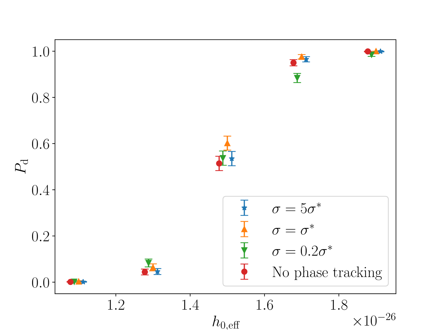
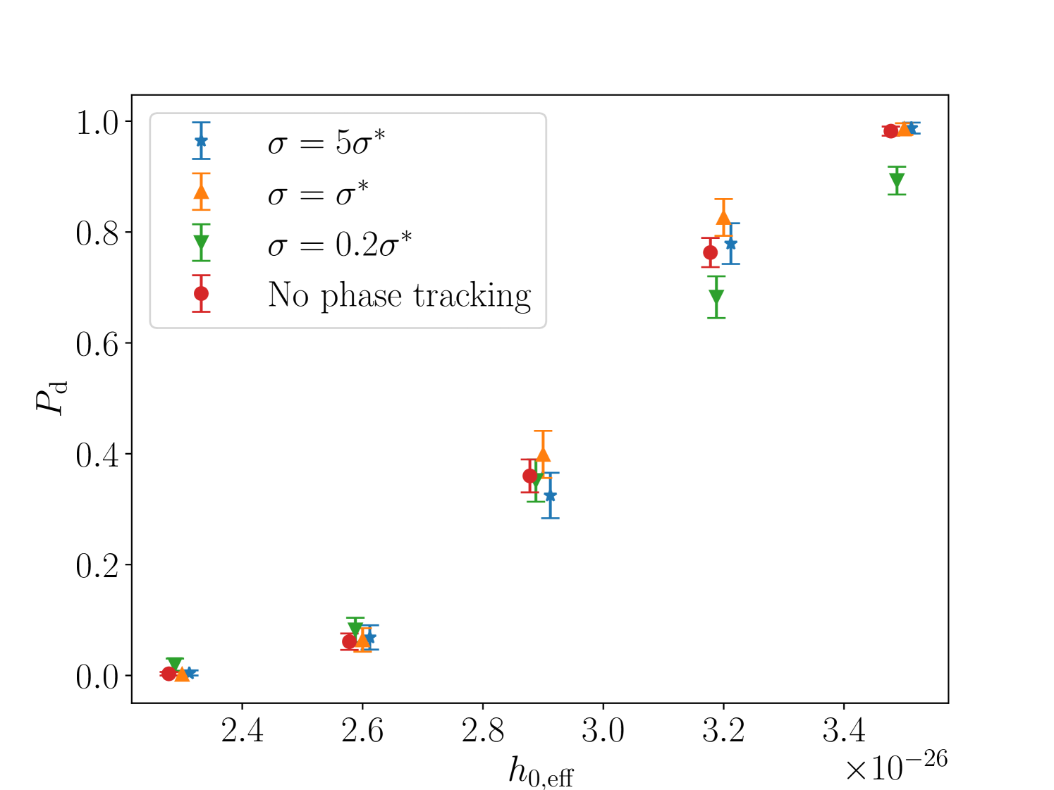
In both cases the choice performs as well as or better than the alternatives as well as no phase tracking across the full range. We adopt throughout the rest of this paper.
III.4.2 Number of phase bins
Another important tunable parameter in the HMM is the number of bins used to track the signal phase, . Melatos et al. [42] fixed . It is worth checking how reducing affects performance. We seek to reduce without sacrificing sensitivity, because the computational cost is proportional to .
To this end we test , , and (c.f. Section III.4.1). Sensitivity curves showing as a function of are displayed in Figure 3.
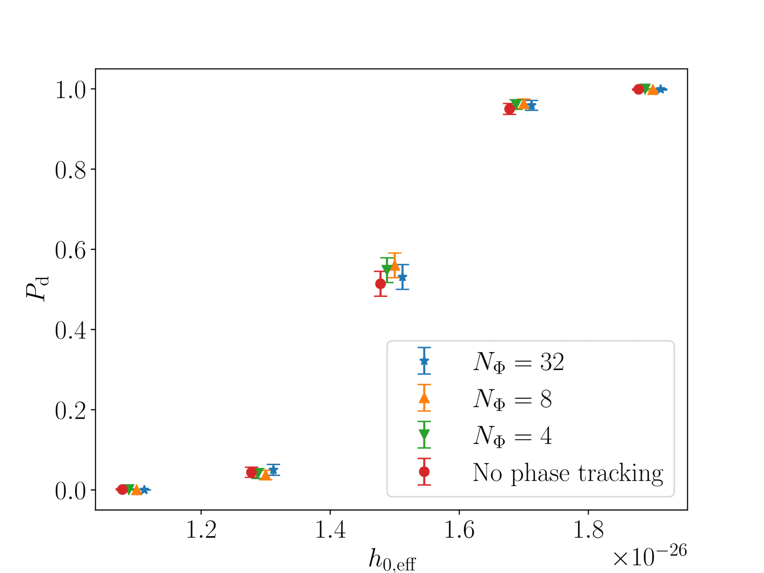
The differences are relatively minor, so we proceed with in what follows.
III.5 Parameter ranges
Ranges must be set for four parameters: the frequency and frequency derivative of the CW signal, and the sky regions covered for each cluster. Here we discuss each in turn, and justify the choices made in the implementation of the search.
III.5.1 Frequency and frequency derivative
In principle the possible frequency of CW emission from neutron stars spans a wide range. Observed pulsar spin frequencies range from less than [90, 91] up to [92]. Although the relationship between the rotation frequency and the CW signal frequency depends on the precise nature of the emission mechanism, one normally assumes [1]. We remind the reader that the notional target for this search is a recycled neutron star, whose rotation frequency is likely to fall between and , as for observed millisecond pulsars. Note that of pulsars above fall in the range [93]. There are also some practical considerations when it comes to selecting the frequency range. The LIGO interferometers are polluted by Newtonian noise below , and narrowband spectral features (instrumental lines) below [94, 95].
The spin-down rate of a CW signal is weakly constrained a priori. Under the optimistic assumption that CW emission is responsible for all of the spindown of the emitting body, the strain amplitude is equal to
| (26) |
where is the component of the moment of inertia tensor about the rotation axis. The expected sensitivity of this search is roughly [56, 78, 96]
| (27) |
which implies for . To beat the spin-down limit we require . We therefore wish to pick a bound on such that the cross-over point occurs at a high enough frequency that we beat the spin-down limit for a significant fraction of plausible signal frequencies. Figure 4 shows the curve with three curves overplotted with , , and . We set in all cases.
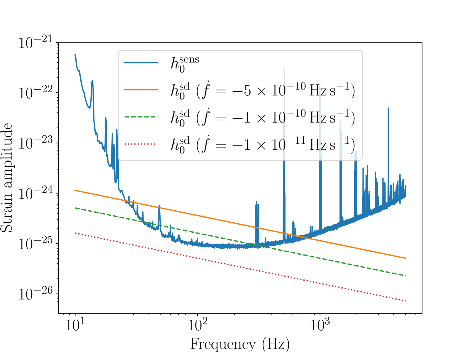
The curve crosses over at approximately . Hence for and we expect to approach or beat the spin-down limit across the full frequency range for each cluster. The range includes the bulk of the astrophysical prior on the signal frequency, recalling that the majority of MSPs have and thus . We therefore adopt and in the present paper. To facilitate data management, the total frequency range is divided into sub-bands which are searched independently.
We note that electromagnetically timed MSPs have spin-down rates orders of magnitude lower than our sensitivity limits according to Fig. 4 [93]. Their spin down is typically attributed to magnetic dipole braking, with the recycling process suppressing the magnetic dipole moment [97, 98, 9, 10, 99, 100]. Hence the signals to which this search is sensitive are most likely to come from a new class of objects with significantly higher spin-down torques, possibly dominated by gravitational radiation reaction [10, 101].
III.5.2 Sky position
Four of the clusters targeted in this search (NGC 6325, NGC 6397, NGC 6544, and Terzan 6) are core-collapsed; their density profiles peak sharply at the core. At the same time, our cluster selection criterion favors clusters which produce disrupted binaries where the neutron star may be ejected from the core. Indeed clusters similar to those selected are observed to contain millisecond pulsars many core radii away from the centre of the cluster [76]. Therefore, as a precaution, we extend the search to cover sky positions outside the core. Specifically, we extend the search out to the tidal radius as recorded in Harris [75], ensuring that every point within this radius is covered by at least one sky position template.
III.6 Parameter spacing
In this paper we search a fairly wide parameter domain (precisely how wide is discussed in Section III.5). In general, multiple templates are needed to cover the domain. In this section we discuss how closely spaced the templates must be. Sophisticated work has been done on this problem in the context of CW searches (e.g. [102, 103, 104, 105]), but we proceed empirically here, because the Viterbi tracking step makes it difficult to apply previous results.
III.6.1 Frequency and frequency derivative
We follow previous HMM-based searches and take the frequency resolution to be . Other choices are possible. In principle any desired frequency resolution may be achieved by padding or decimating the data, e.g. [48, 34], but has been successfully used many times previously (see e.g. Refs. [40, 43, 48, 53, 52]) and is assumed in Eq. (24).
The HMM accommodates some displacement between the value used to compute the -statistic and the true by letting the signal wander into adjacent frequency bins at the boundaries between coherent segments. To determine the resolution we empirically estimate the mismatch, i.e. the fractional loss of signal power which is incurred as the value of used in the search is displaced away from the true value, , with
| (28) |
where we define and is the mean likelihood returned in noise over a sub-band. Note that is the maximum value over a sub-band centred on the injected frequency, and so does not approach but plateaus at approximately , due to the maximisation over noise-only frequency paths (whereas is the mean noise-only value in a sub-band, not the maximum). We compute by injecting moderately loud signals into Gaussian noise, with and . An example of is displayed in Fig. 5, generated from a single realisation of noise and signal. All mismatch curves are smoothed using a Savitzky-Golay filter.
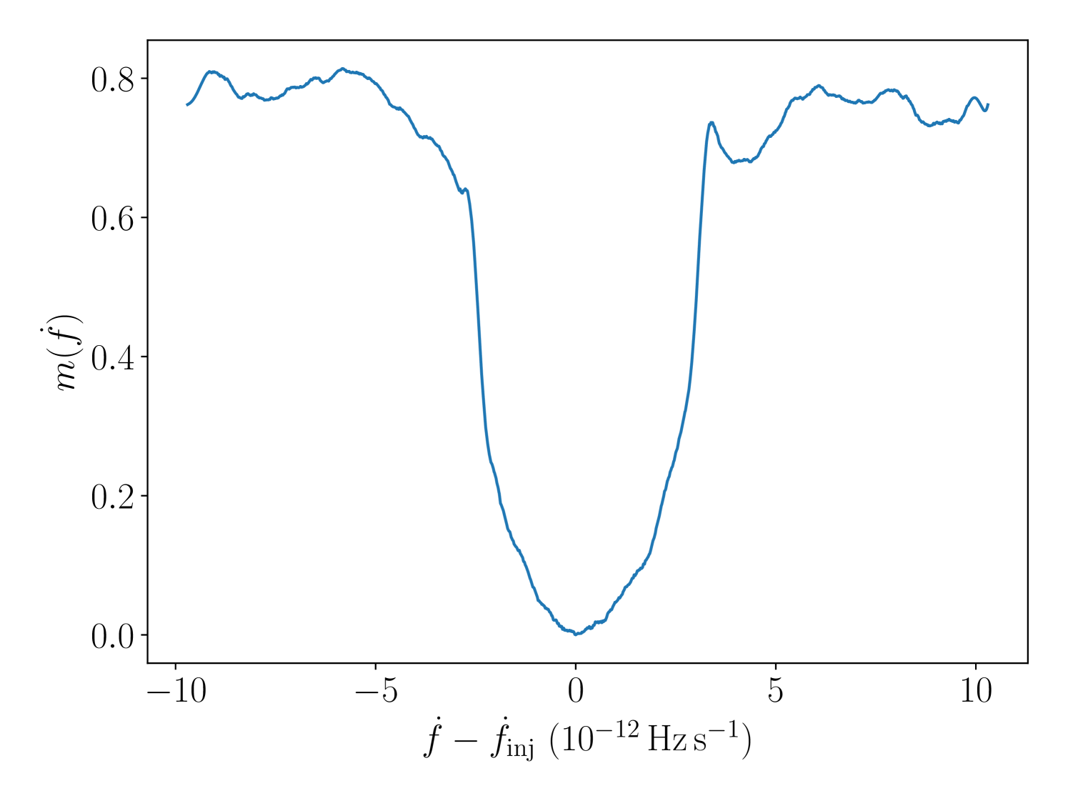
The shape of is consistent across noise realisations. Hence we take the resolution to be the median difference between the two values satisfying , drawn from 100 noise realisations. This gives an resolution of . We verify that the resolution is independent of the injected and values and adopt it throughout the search.
III.6.2 Sky location
A mismatch in sky location induces a small apparent variation in the signal frequency due to a residual Doppler shift. Although the locations of globular clusters are well-known, they are extended objects on the sky. In this search we take a conservative approach and search out to the tidal radius of each cluster, as discussed in Section III.5.2. In general a single sky pointing does not suffice to cover the full sky area of each cluster. As with a mismatch in , we expect the transition matrix in Equation (15) to track some of the residual Doppler variation. Nevertheless it is important to check how much variation can be accommodated before a significant amount of signal power is lost.
We specify the sky location by right ascension () and declination (), referenced to the J2000 epoch. We empirically estimate the mismatch profiles and and thence derive resolutions in and . As with , we smooth the mismatch profiles using a Savitzky-Golay filter. The treatment is somewhat more involved than in Section III.6.1, as and depend on the injected values and as well as , i.e. their shape is not a universal function of sky position offset, because the Doppler modulation varies across the sky. In particular, sky positions at declinations near the ecliptic poles experience relatively little Doppler modulation, and hence proportionally smaller residual Doppler modulations [24]. In this paper, we target five relatively small regions of the sky so we do not produce a full skymap of . Instead we measure the and resolutions independently for each cluster. The clusters themselves are fairly small (diameter ), so we approximate the and resolutions to be uniform within each cluster.
Each cluster is covered by ellipses arranged in a hexagonal grid, with their semimajor and semiminor axes given by the resolutions in and corresponding to and . The centre of one ellipse coincides with the cluster core, and the whole cluster out to the tidal radius is covered by at least one ellipse. The centres of the ellipses are taken as the sky position templates in the search. For simplicity we do not consider degeneracy between sky position and , which may reduce modestly the number of templates, but adds to the complexity of implementing the search.
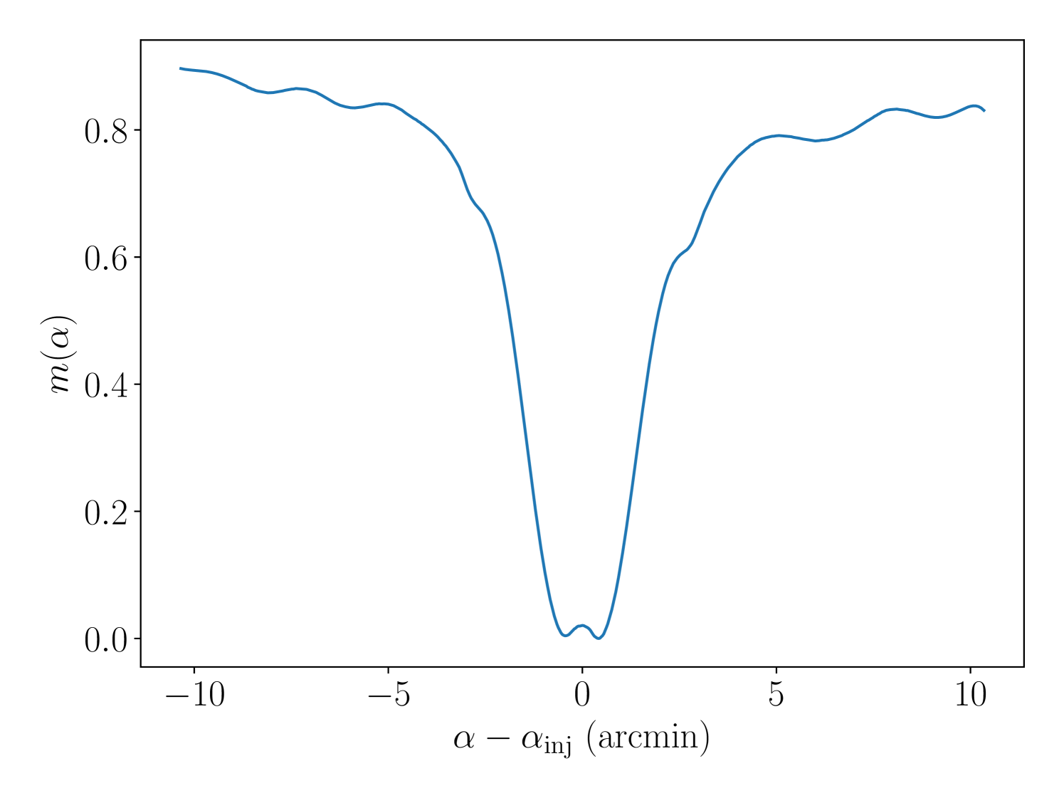
Examples of and are shown in the top two panels of Fig. 6, calculated for Terzan 6 at a frequency of . They are qualitatively similar, with well-defined troughs, but the resolutions, again defined as the distances between the two abcissae where , differ significantly — the resolution inferred from the profile is , compared to for . The bottom panel of 6 shows the measured resolution in and as a function of signal frequency for a series of injections at the sky location of Terzan 6.

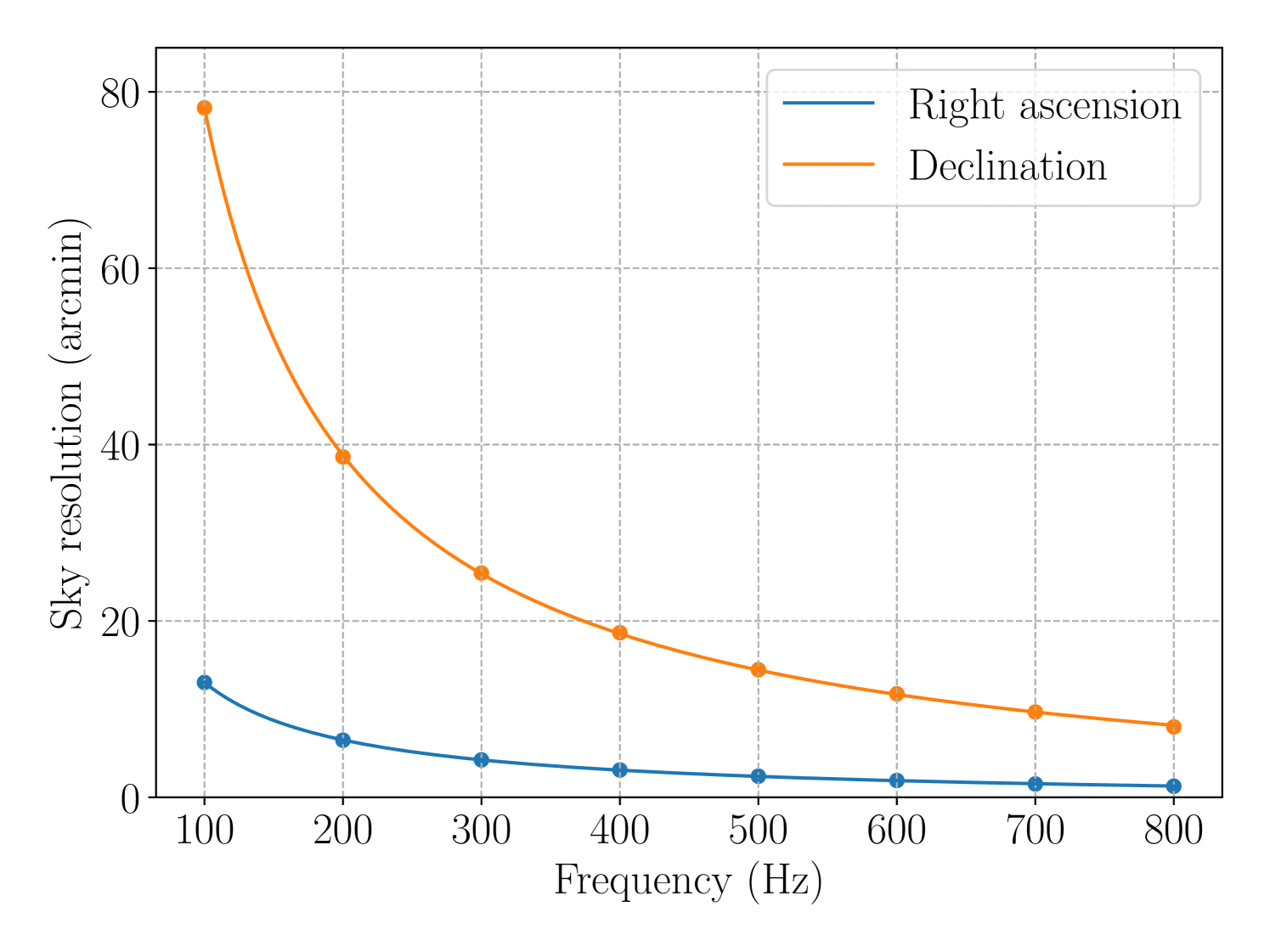
Clearly there is a strong frequency dependence, and it would be wasteful to simply apply the finest resolution across a wide band. Consequently, we produce curves like those in the bottom panel of Fig. 6 for each target. We interpolate by fitting a power-law function for , , and using the lmfit package [106] to find the resolution in each sub-band.
IV Candidates
In this section we present the results of the search. We set the log likelihood threshold in terms of the desired false alarm probaility in Section IV.1. We study the candidates produced by a first-pass analysis in Section IV.2 and apply vetoes to reject those not of astrophysical origin. Finally we study the veto survivors in more depth in Section IV.3.
IV.1 Thresholds
We set a threshold log likelihood above which candidates are kept for further analysis. The threshold is determined by the desired , and is computed according to the procedure outlined in Appendix B. In short, we obtain a sample of values calculated in the absence of a signal, and fit an exponential distribution to the tail of this sample. The exponential distribution is used to calculate the value of that gives the desired . Empirical noise-only distributions of are obtained from random sky pointings in each of three bands beginning at , , and , chosen arbitrarily but checked to ensure that the detector amplitude spectral densities (ASDs) show no obvious spectral artifacts. We find that is similar across the three bands (within of the mean value per cluster), so we take the mean value over the three bands to be as a good approximation. We do not obtain separate noise-only distributions for each cluster.
The choice of is subjective. Historically different searches have used a range of values [24, 39, 33, 48, 53, 52]. In this paper, we take a relatively aggressive approach (i.e. is relatively high), setting on a per-cluster basis such that across all templates in that cluster, we expect one false alarm on average, and so expect the full search to produce five false alarms. This total number of expected false alarms is broadly comparable to other published HMM-based searches, which have adopted values giving false alarm rates ranging from 0.15 per search [48] to 18 per search [53]. The search for CWs from NGC 6544 carried out by Abbott et al. [24] adopted a false alarm rate of 184 per search, while the search targeting Terzan 5 and the galactic center carried out by Dergachev et al. [31] did not set a threshold explicitly in terms of a false alarm rate.
The total number of sky templates and hence differs between clusters. The per-cluster sky template counts and values of corresponding to a false alarm rate of one per cluster are quoted in Table 3.
| Cluster | Sky templates | |
|---|---|---|
| NGC 6544 | 3022 | |
| NGC 6325 | 8416 | |
| NGC 6540 | 8957 | |
| Terzan 6 | 28462 | |
| NGC 6397 | 43909 |
IV.2 First pass candidates and vetoes
The number of above-threshold candidates in each cluster is listed in the pre-veto column of Table 4. The total across all clusters is , with the candidates distributed approximately evenly among the five clusters444For comparison, the total number of Viterbi paths evaluated in this search is approximately .. As discussed in Section IV.2.1, these pre-veto numbers are lower bounds, as most candidates are from heavily disturbed sub-bands and are not saved. The candidate counts in the subsequent columns are complete.
While is far greater than the five expected based on the arguments in Section IV.1, we emphasise that those arguments are based on the assumption that the noise is approximately Gaussian. All but a handful at most of the candidates in the pre-veto column of Table 4 are due to non-Gaussian features in the data. In this section and the next we apply a sequence of veto procedures designed to reject candidates that are consistent with non-Gaussian noise.
IV.2.1 Disturbed sub-band veto
Some of the sub-bands are so disturbed by non-Gaussian artifacts that they are unusable in the absence of noise cancellation [107, 108, 109, 110]. In view of this, we impose a blanket veto on sub-bands which produce output files larger than (corresponding to more than candidates per file). Between % and % of the full search band is removed thus, with the smallest number of removed sub-bands in NGC 6544 (55 out of 1400), and the highest in NGC 6397 (75 out of 1400). These percentages are roughly in line with the all-sky O3a search reported by Abbott et al. [111], for which 13% of the observing band was removed due to an unmanageable number of candidates (noting that the band in that search extended to ). After this veto, approximately candidates remain.
IV.2.2 Known-lines veto
The known-lines veto is simple and efficient, rejecting many candidates with relatively little computational cost. The LIGO Scientific Collaboration maintains a list of known instrumental lines [112, 95]. When assessing coincidence we must take into account that the line frequencies and bandwidths in Ref. [112] are quoted in the detector frame, while the HMM frequency path of a candidate is recorded in the Solar System barycentre frame. The resulting Doppler shift amounts to approximately [113]. For each candidate we check whether any portion of the HMM frequency path overlaps with a known line in either detector, after correcting for the Doppler shift. In the event of any overlap the candidate is vetoed. After this veto, candidates remain.
IV.3 Second pass survivors and vetoes
The survivors from the first pass vetoes are still daunting to follow up manually. We apply three more vetos to further exclude candidates that are consistent with non-Gaussian noise artifacts.
IV.3.1 Cross-cluster veto
The cross-cluster veto excludes candidates which have frequencies overlapping (up to Doppler modulation) with candidates in another cluster. Candidates which appear at the same frequency in multiple clusters are consistent with non-Gaussian noise artifacts.
Given the targeted false alarm rate of one per cluster, we expect five candidate which are due to Gaussian noise fluctuations, and a candidate which overlaps with one of these will be falsely dismissed under this veto. Here we briefly show that the probability of a collision between a Gaussian false alarm and an astrophysical candidate is low. Our criterion for coincidence between two candidates is , where and are the terminal frequencies of the two candidate frequency paths, and is the Doppler broadening factor. To evaluate the probability of a collision, we simulate a search by picking a candidate frequency uniformly over the search range , which is designated as the frequency of the astrophysical candidate, and then pick five more frequencies, again uniformly, which represent the frequencies of the Gaussian false alarm candidates. We then check the coincidence criterion for each Gaussian false alarm against the astrophysical candidate. Simulating searches in this way, we find collisions, i.e. the probability of falsely dismissing an astrophysical candidate due to coincidence with a Gaussian false alarm is approximately , which we find to be acceptably low. We therefore veto any candidate for which there is a candidate in another cluster with respective frequencies and satisfying .
candidates are vetoed this way. We find that all of the vetoed candidates have at least 4 cross-cluster counterparts, i.e. distinct combinations of , , and with at least one frequency path with overlapping with the vetoed candidate — multiple cross-cluster counterparts may be associated with the same cluster. After this veto, candidates remain.
IV.3.2 Single-interferometer veto
If a candidate is due to a non-Gaussian feature which is present in the data from only one interferometer, we expect the significance of the candidate to increase when data from only that interferometer is used. We thus veto candidates satisfying , where is the log likelihood of the candidate template using only data from detector and is the log likelihood computed using data from both detectors. Before carrying out this veto we group candidates that have frequencies within of each other, in order to reduce the computation required and enable manual verification of the results of the veto procedure. There are 10 candidate groups in total, appearing in two clusters, NGC 6397 and NGC 6544. To compute over the relevant frequency band we use the loudest sky position and template in each candidate group, and is taken to be the loudest log likelihood value in the candidate group. Plots showing in comparison to for each candidate are collected in Appendix C. In all but one case, one value peaks above , indicating that the candidate group is likely to be due to a disturbance in the corresponding interferometer and is not astrophysical. These candidate groups are vetoed.
After the single-interferometer veto, two candidates remain.
IV.3.3 Unknown lines veto
The line list used for the known-lines veto [112] includes only lines for which there is good evidence of a non-astrophysical origin. Other line-like features are visible by eye in plots of the detector ASDs but have not yet been confidently associated with a terrestrial source.
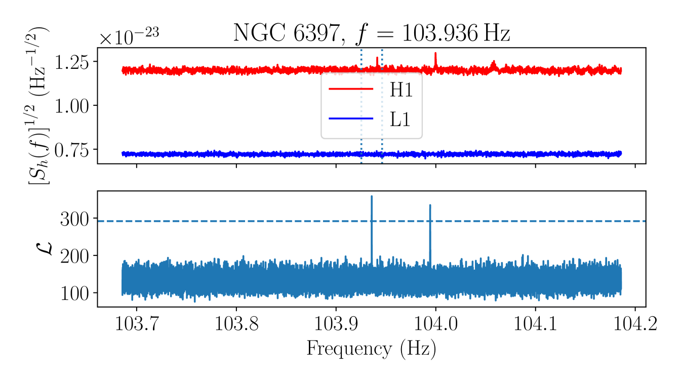
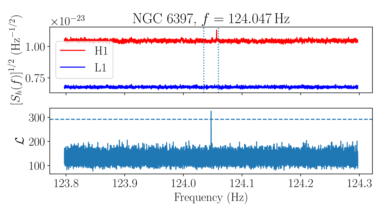
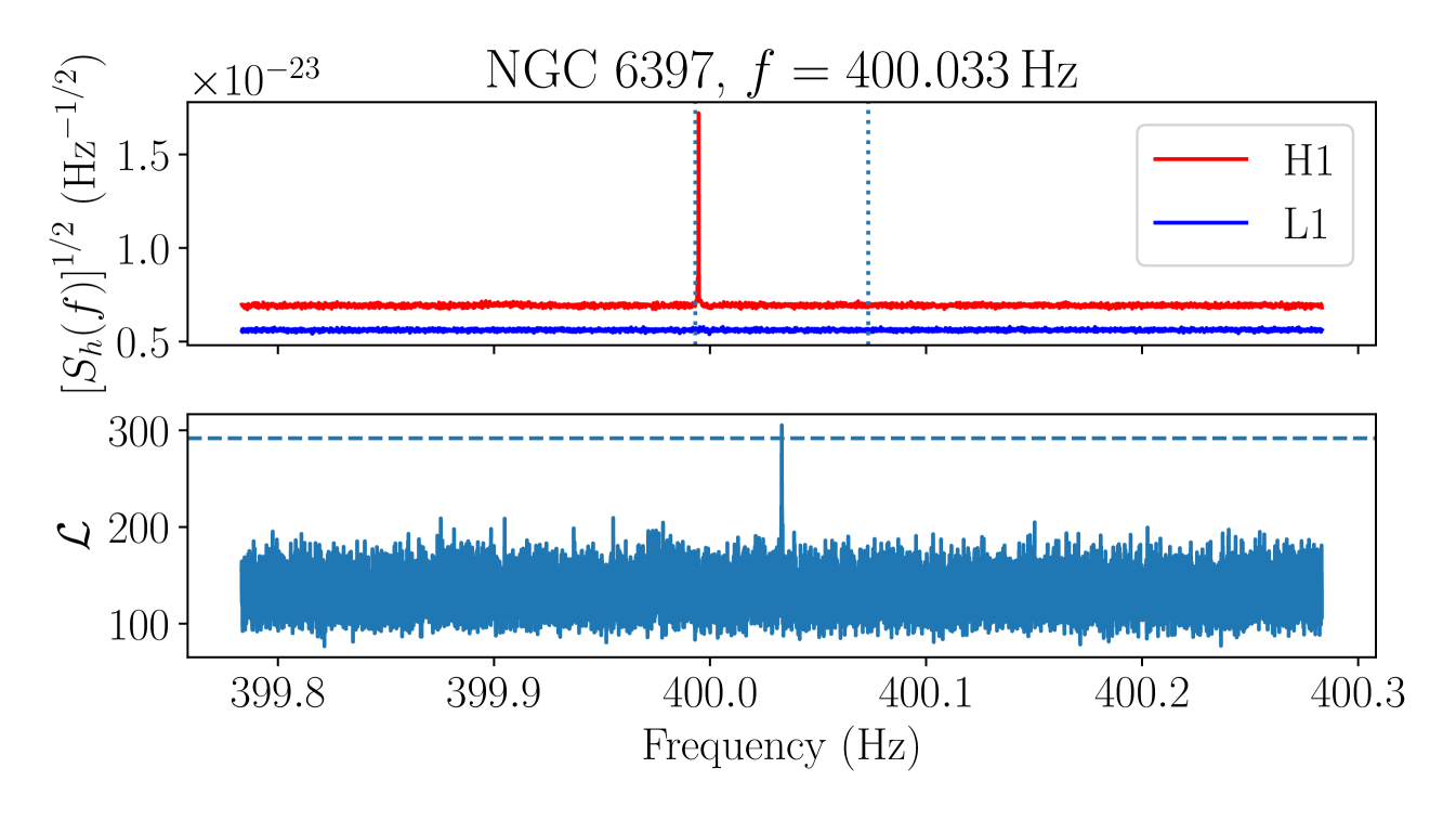
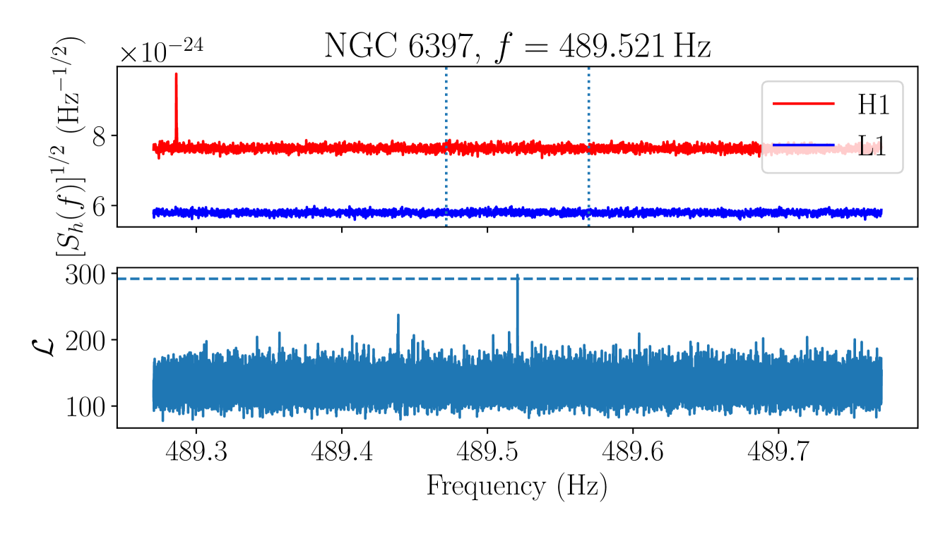
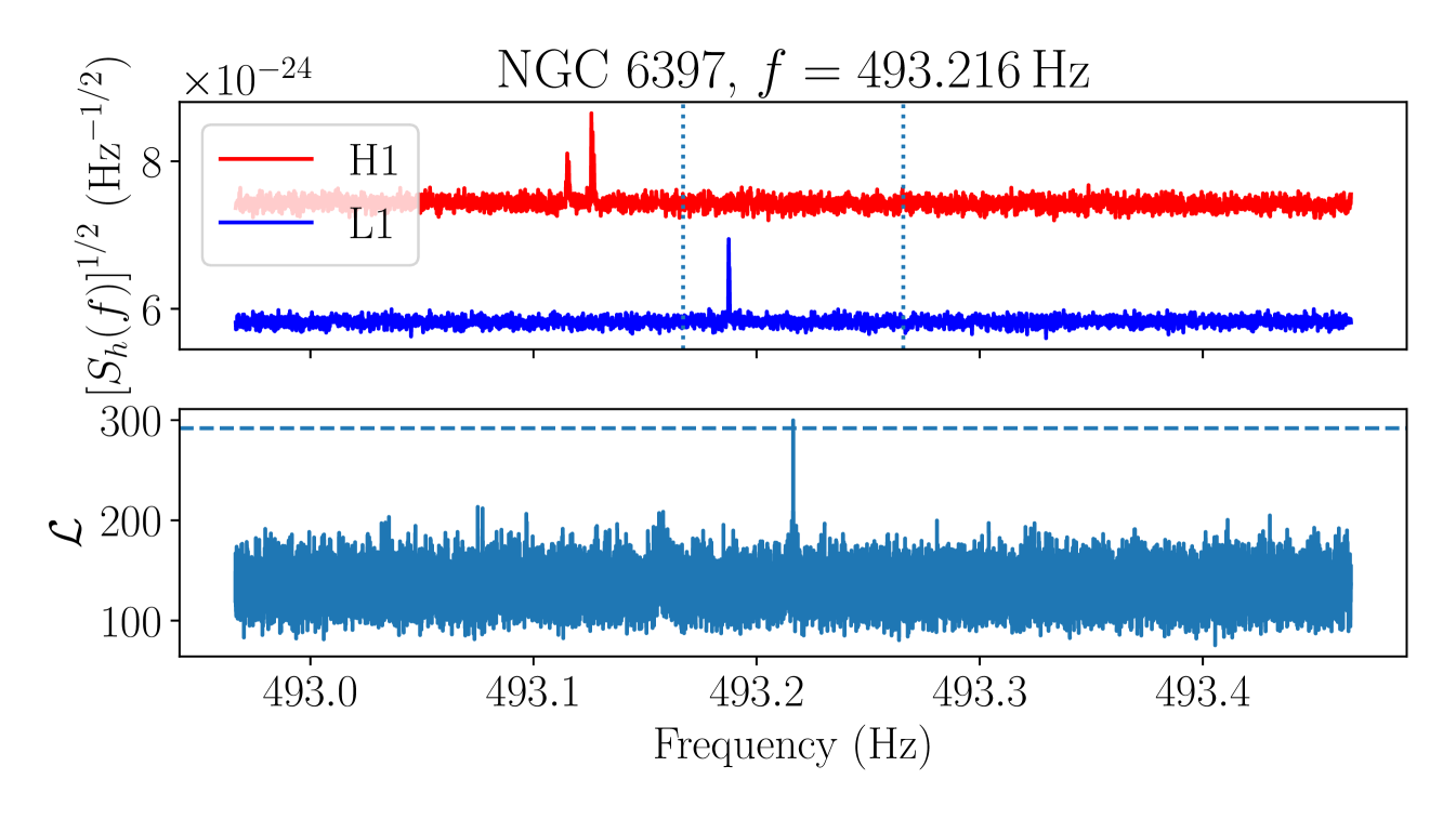
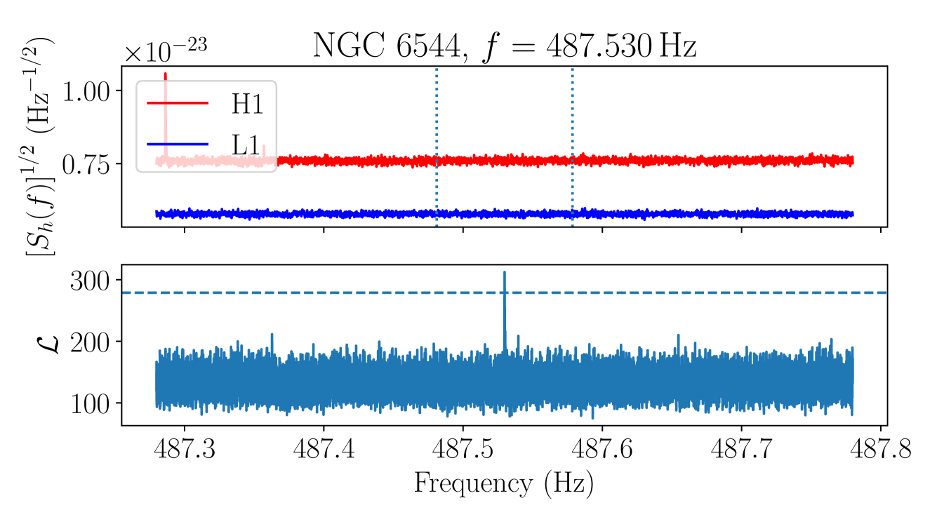
As a further check on the final remaining candidate group, we manually inspect the ASD in each detector to check whether the candidate group overlaps with a loud non-Gaussian feature in the data, taking into account the Doppler modulation. Candidates which overlap with a clear feature in an ASD are vetoed, on the grounds that we expect any astrophysical signal to be at most marginally visible in the detector ASDs at distances [114]. A plot showing the detector ASDs and corresponding values for the loudest candidate in the remaining candidate group, in the cluster NGC at , is shown in Figure 7.
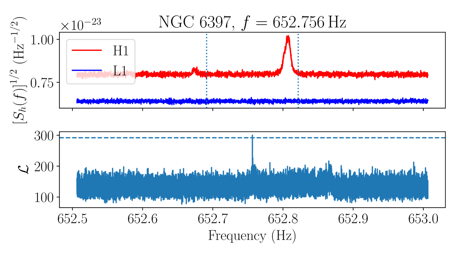
There is a clear, broad peak in the H1 ASD within the Doppler modulation range of the candidate, with no corresponding feature visible in the L1 ASD. We therefore veto this candidate group.
After the unknown lines veto, no candidates remain.
IV.4 Summary of vetoes
After applying the veto procedures described in Sections IV.2 and IV.3, we are left with no surviving candidates. A summary of the results of the veto procedures is given in Table 4.
| Cluster | Pre-veto | DS | KL | CC | 1IFO | UL |
|---|---|---|---|---|---|---|
| NGC 6544 | ||||||
| NGC 6325 | ||||||
| NGC 6540 | ||||||
| Terzan 6 | ||||||
| NGC 6397 | ||||||
| Total |
The disturbed sub-band and known-lines vetos reject most of the candidates but leave , still a significant number. The cross-cluster veto further rejects all but candidates, which are grouped into ten narrow frequency bands. We find that for nine of the ten groups, one of the single-detector log likelihoods peaks at a higher value than the joint-detector peak, indicating that these candidates are due to a non-Gaussian feature which is peculiar to one detector. Hence these groups are vetoed. The remaining group is in the vicinity of a broad, loud disturbance in the H1 detector and is therefore also vetoed.
V Sensitivity
In this section we estimate the sensitivity of the search to CW emission from each targeted globular cluster. Specifically, for each cluster we estimate , the effective strain amplitude [defined in Eq. (25)] at which we would expect to detect a signal 95% of the time. We draw the distinction between the search sensitivity, defined as above, and an upper limit. An upper limit is a limit on the loudest astrophysical signal actually present in the data, and is necessarily estimated with reference to the results of the search (i.e. estimation of the upper limit in a given sub-band depends on the loudest candidate in that sub-band). By contrast the search sensitivity is not a function of the results of the search, only the search configuration. We prefer to estimate the search sensitivity here as it is straightforward to interpret and requires less computation. Computing upper limits requires estimating a relationship between the noise ASD in a given sub-band, , the log likelihood of the loudest candidate in that sub-band, , and the effective strain amplitude which produces a candidate at least that loud 95% of the time, . This can be done, of course, but it is more involved and requires costly signal injection studies. Here we estimate the search sensitivity in a small number of sub-bands and subsequently interpolate across the full search band, as described below.
In order to estimate the search sensitivity we inject synthetic signals into the real O3 data. We inject at sky positions slightly offset in right ascension from the true cluster position, so that the sky templates do not overlap with the search, so as to avoid the possibility of contamination by an astrophysical signal from the cluster.In a given sub-band we inject signals at ten evenly spaced levels between and and determine the detection rate as a function of . We then fit these rates as a function of to a sigmoid curve, following Abbott et al. [48]. We use the best-fit parameters to determine the value yielding , in that sub-band.
The off-target injections and recoveries are treated much the same as in the actual search. The key difference is that the centre of the injection-containing mock cluster is offset from the true cluster centre by five tidal radii in right ascension. The placement of , , and templates mimics that of the real search, but to save computational resources we only search templates within of the injected . We also search a reduced frequency range around the injection frequency. The value of is the same as in the real search555In the searches around these mock injections the number of templates is smaller than the number used in real searches, implying a smaller for the targeted false alarm rate. Nonetheless the aim is to ascertain the sensitivity of the real searches, and so we use the values quoted in Table 3., and we claim a successful recovery if the maximum recovered value of exceeds regardless of which template returns the maximum. As we set on a per-cluster basis (see Section IV.1), we expect different sensitivity curves for each cluster, with clusters requiring fewer sky position templates (and hence smaller values) reaching deeper sensitivities.
We determine the value of directly following the above recipe in a small number of bands (beginning at , , , , , and ) and then interpolate to cover the full observing band. The value of is a strong function of frequency, but to a good approximation it is directly proportional to the detector-averaged ASD . Therefore in order to interpolate the estimated values in the six sub-bands to a curve which covers the entire observing band we estimate the sensitivity depth , which is the constant of proportionality between and and is defined as
| (29) |
We compute using lalpulsar_ComputePSD, averaging over all data used in the search from both detectors. There is some scatter in the computed values in the six sub-bands, with for each cluster, where is the mean value of across the six sub-bands. There is no clear trend in as a function of frequency. As is defined to be the constant of proportionality between and , to obtain a curve of for each cluster over the full band we divide by the value for that cluster.
The resulting sensitivity curves are shown in the top panel of Figure 8.
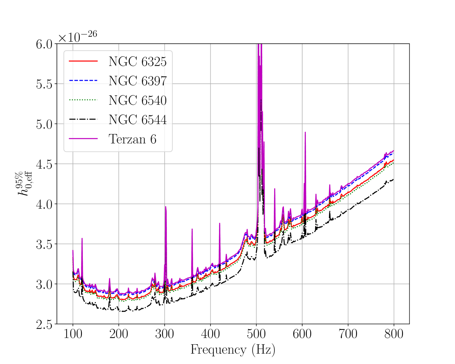
The values used to produce the curves are listed in Table 5.
| Cluster | |
|---|---|
| Terzan 6 | 116.3 |
| NGC 6397 | 117.0 |
| NGC 6325 | 119.3 |
| NGC 6540 | 120.2 |
| NGC 6544 | 125.9 |
The differences in sensitivity between the five clusters are due to the varying values for each cluster (see Table 3), which follow from the number of sky position templates (see Sections III.5.2 and III.6.2). The variation between clusters is fairly small: the least sensitive cluster (Terzan 6) is approximately 10% worse than the most sensitive (NGC 6544), achieving and respectively at the most sensitive frequency of .
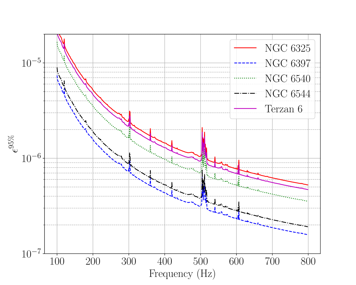
Out of astrophysical interest, we also convert in Figure 8 into estimates of the minimum ellipticity of a source which would have been detected by this search assuming emission at twice the rotational frequency, according to the relation [51]
| (30) |
Curves of versus signal frequency for the five clusters are shown in the bottom panel of Figure 8. The smallest minimum ellipticity estimates are achieved at the top of the observing band, , due to the factor in Eq. (30). The factor of introduces larger variation between the clusters compared to the variation in values, and modifies the relative ordering — the smallest minimum ellipticity estimate is , for the nearest cluster NGC 6397 (), while the largest is for the farthest cluster NGC 6325 ().
VI Conclusion
We carry out a search for continuous gravitational radiation from unknown neutron stars in five globular clusters. This is the first time that all but one of the chosen clusters have been targeted. For NGC 6544 which was previously searched using LIGO S6 data, the sensitivity is improved approximately one order of magnitude [24] (although note that the signal models and parameter domain differ, so a direct, like-for-like comparison is impossible). This is also the first search to use a phase-tracking HMM in conjunction with a phase-dependent version of the -statistic [59, 42]; previous HMM searches tracked frequency only, not phase. Phase tracking brings with it an increase in sensitivity, but also increases the computational cost. For searches aiming to optimize sensitivity at fixed computing cost, a careful analysis of the tradeoff between sensitivity and cost is crucial. We do not undertake this exercise in this paper, as a key aim is to demonstrate the use of the phase-tracking HMM in an astrophysical search for the first time.
We find no significant candidates. We estimate the effective strain amplitude sensitivity for each cluster, along with a corresponding estimate of the ellipticity sensitivity. The minimum per-cluster values of lie in the range , achieved at approximately , while the minimum values of are achieved at the top end of the search band (), and lie in the range . The lowest values are obtained for the cluster NGC 6544, while the lowest values are obtained for NGC 6397.
We surpass the spin-down limit for , with variation between clusters due primarily to the difference in distance. As discussed in Section III.5, electromagnetically visible MSPs have spin-down rates well below this limit, so this search is primarily sensitive to “gravitars” — neutron stars whose spin-down behaviour is dominated by gravitational rather than electromagnetic torques [101]. The inferred limits on the ellipticity of the star probe up to an order of magnitude below theoretical upper limits, viz. [115, 116].
Acknowledgments
Parts of this research are supported by the Australian Research Council (ARC) Centre of Excellence for Gravitational Wave Discovery (OzGrav) (project numbers CE170100004 and CE230100016) and ARC Discovery Project DP170103625. This material is based upon work supported by NSF’s LIGO Laboratory which is a major facility fully funded by the National Science Foundation. LD is supported by an Australian Government Research Training Program Scholarship. LS is supported by the ARC Discovery Early Career Researcher Award, Project Number DE240100206. This work was performed in part on the OzSTAR national facility at Swinburne University of Technology. The OzSTAR program receives funding in part from the Astronomy National Collaborative Research Infrastructure Strategy allocation provided by the Australian Government.
References
- Riles [2023] K. Riles, Searches for continuous-wave gravitational radiation, Living Reviews in Relativity 26, 3 (2023), arXiv:2206.06447 [astro-ph.HE] .
- Wette [2023] K. Wette, Searches for continuous gravitational waves from neutron stars: A twenty-year retrospective, Astroparticle Physics 153, 102880 (2023), arXiv:2305.07106 [gr-qc] .
- Bildsten [1998] L. Bildsten, Gravitational Radiation and Rotation of Accreting Neutron Stars, The Astrophysical Journal 501, L89 (1998), arXiv:astro-ph/9804325 [astro-ph] .
- Ushomirsky et al. [2000] G. Ushomirsky, C. Cutler, and L. Bildsten, Deformations of accreting neutron star crusts and gravitational wave emission, Monthly Notices of the Royal Astronomical Society 319, 902 (2000), arXiv:astro-ph/0001136 [astro-ph] .
- Osborne and Jones [2020] E. L. Osborne and D. I. Jones, Gravitational waves from magnetically induced thermal neutron star mountains, Monthly Notices of the Royal Astronomical Society 494, 2839 (2020), arXiv:1910.04453 [astro-ph.HE] .
- Hutchins and Jones [2023] T. J. Hutchins and D. I. Jones, Gravitational radiation from thermal mountains on accreting neutron stars: sources of temperature non-axisymmetry, Monthly Notices of the Royal Astronomical Society 522, 226 (2023), arXiv:2212.07452 [astro-ph.HE] .
- Bonazzola and Gourgoulhon [1996] S. Bonazzola and E. Gourgoulhon, Gravitational waves from pulsars: emission by the magnetic-field-induced distortion., Astronomy and Astrophysics 312, 675 (1996), arXiv:astro-ph/9602107 [astro-ph] .
- Cutler [2002] C. Cutler, Gravitational waves from neutron stars with large toroidal B fields, Physical Review D 66, 084025 (2002), arXiv:gr-qc/0206051 [gr-qc] .
- Payne and Melatos [2004] D. J. B. Payne and A. Melatos, Burial of the polar magnetic field of an accreting neutron star - I. Self-consistent analytic and numerical equilibria, Monthly Notices of the Royal Astronomical Society 351, 569 (2004), arXiv:astro-ph/0403173 [astro-ph] .
- Melatos and Payne [2005] A. Melatos and D. J. B. Payne, Gravitational Radiation from an Accreting Millisecond Pulsar with a Magnetically Confined Mountain, The Astrophysical Journal 623, 1044 (2005), arXiv:astro-ph/0503287 [astro-ph] .
- Payne and Melatos [2006] D. J. B. Payne and A. Melatos, Frequency Spectrum of Gravitational Radiation from Global Hydromagnetic Oscillations of a Magnetically Confined Mountain on an Accreting Neutron Star, The Astrophysical Journal 641, 471 (2006), arXiv:astro-ph/0510053 [astro-ph] .
- Rossetto et al. [2023] P. H. B. Rossetto, J. Frauendiener, R. Brunet, and A. Melatos, Magnetically confined mountains on accreting neutron stars in general relativity, Monthly Notices of the Royal Astronomical Society 526, 2058 (2023), arXiv:2309.09519 [astro-ph.HE] .
- Caplan and Horowitz [2017] M. E. Caplan and C. J. Horowitz, Colloquium: Astromaterial science and nuclear pasta, Reviews of Modern Physics 89, 041002 (2017), arXiv:1606.03646 [astro-ph.HE] .
- Gittins et al. [2021] F. Gittins, N. Andersson, and D. I. Jones, Modelling neutron star mountains, Monthly Notices of the Royal Astronomical Society 500, 5570 (2021), arXiv:2009.12794 [astro-ph.HE] .
- Kerin and Melatos [2022] A. D. Kerin and A. Melatos, Mountain formation by repeated, inhomogeneous crustal failure in a neutron star, Monthly Notices of the Royal Astronomical Society 514, 1628 (2022), arXiv:2205.15026 [astro-ph.HE] .
- Andersson et al. [1999] N. Andersson, K. D. Kokkotas, and N. Stergioulas, On the Relevance of the R-Mode Instability for Accreting Neutron Stars and White Dwarfs, The Astrophysical Journal 516, 307 (1999), arXiv:astro-ph/9806089 [astro-ph] .
- Arras et al. [2003] P. Arras, E. E. Flanagan, S. M. Morsink, A. K. Schenk, S. A. Teukolsky, and I. Wasserman, Saturation of the r-Mode Instability, The Astrophysical Journal 591, 1129 (2003), arXiv:astro-ph/0202345 [astro-ph] .
- Bondarescu et al. [2007] R. Bondarescu, S. A. Teukolsky, and I. Wasserman, Spin evolution of accreting neutron stars: Nonlinear development of the r-mode instability, Physical Review D 76, 064019 (2007), arXiv:0704.0799 [astro-ph] .
- Katz [1975] J. I. Katz, Two kinds of stellar collapse, Nature 253, 698 (1975).
- Clark [1975] G. W. Clark, X-ray binaries in globular clusters., The Astrophysical Journal 199, L143 (1975).
- Alpar et al. [1982] M. A. Alpar, A. F. Cheng, M. A. Ruderman, and J. Shaham, A new class of radio pulsars, Nature 300, 728 (1982).
- Pooley et al. [2003] D. Pooley, W. H. G. Lewin, S. F. Anderson, H. Baumgardt, A. V. Filippenko, B. M. Gaensler, L. Homer, P. Hut, V. M. Kaspi, J. Makino, B. Margon, S. McMillan, S. Portegies Zwart, M. van der Klis, and F. Verbunt, Dynamical Formation of Close Binary Systems in Globular Clusters, The Astrophysical Journal 591, L131 (2003), arXiv:astro-ph/0305003 [astro-ph] .
- Wang et al. [2006] Z. Wang, D. Chakrabarty, and D. L. Kaplan, A debris disk around an isolated young neutron star, Nature 440, 772 (2006), arXiv:astro-ph/0604076 [astro-ph] .
- Abbott et al. [2017a] B. P. Abbott, R. Abbott, T. D. Abbott, M. R. Abernathy, F. Acernese, K. Ackley, C. Adams, T. Adams, P. Addesso, R. X. Adhikari, and et al., Search for continuous gravitational waves from neutron stars in globular cluster NGC 6544, Physical Review D 95, 082005 (2017a), arXiv:1607.02216 [gr-qc] .
- Jennings et al. [2020] R. J. Jennings, J. M. Cordes, and S. Chatterjee, Pulsar Timing Signatures of Circumbinary Asteroid Belts, The Astrophysical Journal 904, 191 (2020), arXiv:2007.10388 [astro-ph.HE] .
- Wolszczan and Frail [1992] A. Wolszczan and D. A. Frail, A planetary system around the millisecond pulsar PSR1257 + 12, Nature 355, 145 (1992).
- Bailes et al. [2011] M. Bailes, S. D. Bates, V. Bhalerao, N. D. R. Bhat, M. Burgay, S. Burke-Spolaor, N. D’Amico, S. Johnston, M. J. Keith, M. Kramer, S. R. Kulkarni, L. Levin, A. G. Lyne, S. Milia, A. Possenti, L. Spitler, B. Stappers, and W. van Straten, Transformation of a Star into a Planet in a Millisecond Pulsar Binary, Science 333, 1717 (2011), arXiv:1108.5201 [astro-ph.SR] .
- Spiewak et al. [2018] R. Spiewak, M. Bailes, E. D. Barr, N. D. R. Bhat, M. Burgay, A. D. Cameron, D. J. Champion, C. M. L. Flynn, A. Jameson, S. Johnston, M. J. Keith, M. Kramer, S. R. Kulkarni, L. Levin, A. G. Lyne, V. Morello, C. Ng, A. Possenti, V. Ravi, B. W. Stappers, W. van Straten, and C. Tiburzi, PSR J2322-2650 - a low-luminosity millisecond pulsar with a planetary-mass companion, Monthly Notices of the Royal Astronomical Society 475, 469 (2018), arXiv:1712.04445 [astro-ph.HE] .
- Behrens et al. [2020] E. A. Behrens, S. M. Ransom, D. R. Madison, Z. Arzoumanian, K. Crowter, M. E. DeCesar, P. B. Demorest, T. Dolch, J. A. Ellis, R. D. Ferdman, E. C. Ferrara, E. Fonseca, P. A. Gentile, G. Jones, M. L. Jones, M. T. Lam, L. Levin, D. R. Lorimer, R. S. Lynch, M. A. McLaughlin, C. Ng, D. J. Nice, T. T. Pennucci, B. B. P. Perera, P. S. Ray, R. Spiewak, I. H. Stairs, K. Stovall, J. K. Swiggum, and W. W. Zhu, The NANOGrav 11 yr Data Set: Constraints on Planetary Masses Around 45 Millisecond Pulsars, The Astrophysical Journal 893, L8 (2020), arXiv:1912.00482 [astro-ph.EP] .
- Niţu et al. [2022] I. C. Niţu, M. J. Keith, B. W. Stappers, A. G. Lyne, and M. B. Mickaliger, A search for planetary companions around 800 pulsars from the Jodrell Bank pulsar timing programme, Monthly Notices of the Royal Astronomical Society 512, 2446 (2022), arXiv:2203.01136 [astro-ph.EP] .
- Dergachev et al. [2019] V. Dergachev, M. A. Papa, B. Steltner, and H.-B. Eggenstein, Loosely coherent search in LIGO O1 data for continuous gravitational waves from Terzan 5 and the Galactic Center, Physical Review D 99, 084048 (2019), arXiv:1903.02389 [gr-qc] .
- Aasi et al. [2013] J. Aasi, J. Abadie, B. P. Abbott, R. Abbott, T. Abbott, M. R. Abernathy, T. Accadia, F. Acernese, C. Adams, T. Adams, and et al., Directed search for continuous gravitational waves from the Galactic center, Physical Review D 88, 102002 (2013), arXiv:1309.6221 [gr-qc] .
- Piccinni et al. [2020] O. J. Piccinni, P. Astone, S. D’Antonio, S. Frasca, G. Intini, I. La Rosa, P. Leaci, S. Mastrogiovanni, A. Miller, and C. Palomba, Directed search for continuous gravitational-wave signals from the Galactic Center in the Advanced LIGO second observing run, Physical Review D 101, 082004 (2020), arXiv:1910.05097 [gr-qc] .
- Abbott et al. [2022a] R. Abbott, H. Abe, F. Acernese, K. Ackley, N. Adhikari, R. X. Adhikari, V. K. Adkins, V. B. Adya, C. Affeldt, D. Agarwal, and et al., Search for continuous gravitational wave emission from the Milky Way center in O3 LIGO-Virgo data, Physical Review D 106, 042003 (2022a), arXiv:2204.04523 [astro-ph.HE] .
- Abbott et al. [2010] B. P. Abbott, R. Abbott, F. Acernese, R. Adhikari, P. Ajith, B. Allen, G. Allen, M. Alshourbagy, R. S. Amin, S. B. Anderson, and et al., Searches for Gravitational Waves from Known Pulsars with Science Run 5 LIGO Data, The Astrophysical Journal 713, 671 (2010), arXiv:0909.3583 [astro-ph.HE] .
- Aasi et al. [2014] J. Aasi, J. Abadie, B. P. Abbott, R. Abbott, T. Abbott, M. R. Abernathy, T. Accadia, F. Acernese, C. Adams, T. Adams, and et al., Gravitational Waves from Known Pulsars: Results from the Initial Detector Era, The Astrophysical Journal 785, 119 (2014), arXiv:1309.4027 [astro-ph.HE] .
- Pitkin et al. [2015] M. Pitkin, C. Gill, D. I. Jones, G. Woan, and G. S. Davies, First results and future prospects for dual-harmonic searches for gravitational waves from spinning neutron stars, Monthly Notices of the Royal Astronomical Society 453, 4399 (2015), arXiv:1508.00416 [astro-ph.HE] .
- Abbott et al. [2017b] B. P. Abbott, R. Abbott, T. D. Abbott, M. R. Abernathy, F. Acernese, K. Ackley, C. Adams, T. Adams, P. Addesso, R. X. Adhikari, and et al., First Search for Gravitational Waves from Known Pulsars with Advanced LIGO, The Astrophysical Journal 839, 12 (2017b), arXiv:1701.07709 [astro-ph.HE] .
- Abbott et al. [2019a] B. P. Abbott, R. Abbott, T. D. Abbott, S. Abraham, F. Acernese, K. Ackley, C. Adams, R. X. Adhikari, V. B. Adya, C. Affeldt, and et al., All-sky search for continuous gravitational waves from isolated neutron stars using Advanced LIGO O2 data, Physical Review D 100, 024004 (2019a), arXiv:1903.01901 [astro-ph.HE] .
- Suvorova et al. [2016] S. Suvorova, L. Sun, A. Melatos, W. Moran, and R. J. Evans, Hidden Markov model tracking of continuous gravitational waves from a neutron star with wandering spin, Physical Review D 93, 123009 (2016), arXiv:1606.02412 [astro-ph.IM] .
- Suvorova et al. [2018] S. Suvorova, A. Melatos, R. J. Evans, W. Moran, P. Clearwater, and L. Sun, Phase-Continuous Frequency Line Track-Before-Detect of a Tone With Slow Frequency Variation, IEEE Transactions on Signal Processing 66, 6434 (2018).
- Melatos et al. [2021] A. Melatos, P. Clearwater, S. Suvorova, L. Sun, W. Moran, and R. J. Evans, Hidden Markov model tracking of continuous gravitational waves from a binary neutron star with wandering spin. III. Rotational phase tracking, Physical Review D 104, 042003 (2021), arXiv:2107.12822 [gr-qc] .
- Abbott et al. [2017c] B. P. Abbott, R. Abbott, T. D. Abbott, F. Acernese, K. Ackley, C. Adams, T. Adams, P. Addesso, R. X. Adhikari, V. B. Adya, and et al., Search for gravitational waves from Scorpius X-1 in the first Advanced LIGO observing run with a hidden Markov model, Physical Review D 95, 122003 (2017c), arXiv:1704.03719 [gr-qc] .
- Abbott et al. [2019b] B. P. Abbott, R. Abbott, T. D. Abbott, S. Abraham, F. Acernese, K. Ackley, C. Adams, R. X. Adhikari, V. B. Adya, C. Affeldt, and et al., Search for gravitational waves from Scorpius X-1 in the second Advanced LIGO observing run with an improved hidden Markov model, Physical Review D 100, 122002 (2019b), arXiv:1906.12040 [gr-qc] .
- Millhouse et al. [2020] M. Millhouse, L. Strang, and A. Melatos, Search for gravitational waves from 12 young supernova remnants with a hidden Markov model in Advanced LIGO’s second observing run, Physical Review D 102, 083025 (2020), arXiv:2003.08588 [gr-qc] .
- Middleton et al. [2020] H. Middleton, P. Clearwater, A. Melatos, and L. Dunn, Search for gravitational waves from five low mass x-ray binaries in the second Advanced LIGO observing run with an improved hidden Markov model, Physical Review D 102, 023006 (2020), arXiv:2006.06907 [astro-ph.HE] .
- Sun et al. [2020a] L. Sun, R. Brito, and M. Isi, Search for ultralight bosons in Cygnus X-1 with Advanced LIGO, Physical Review D 101, 063020 (2020a), arXiv:1909.11267 [gr-qc] .
- Abbott et al. [2021a] R. Abbott, T. D. Abbott, S. Abraham, F. Acernese, K. Ackley, A. Adams, C. Adams, R. X. Adhikari, V. B. Adya, C. Affeldt, and et al., Searches for Continuous Gravitational Waves from Young Supernova Remnants in the Early Third Observing Run of Advanced LIGO and Virgo, The Astrophysical Journal 921, 80 (2021a), arXiv:2105.11641 [astro-ph.HE] .
- Jones and Sun [2021] D. Jones and L. Sun, Search for continuous gravitational waves from Fomalhaut b in the second Advanced LIGO observing run with a hidden Markov model, Physical Review D 103, 023020 (2021), arXiv:2007.08732 [gr-qc] .
- Beniwal et al. [2021] D. Beniwal, P. Clearwater, L. Dunn, A. Melatos, and D. Ottaway, Search for continuous gravitational waves from ten H.E.S.S. sources using a hidden Markov model, Physical Review D 103, 083009 (2021), arXiv:2102.06334 [astro-ph.HE] .
- Beniwal et al. [2022] D. Beniwal, P. Clearwater, L. Dunn, L. Strang, G. Rowell, A. Melatos, and D. Ottaway, Search for continuous gravitational waves from HESS J1427-608 with a hidden Markov model, Physical Review D 106, 103018 (2022), arXiv:2210.09592 [astro-ph.HE] .
- Abbott et al. [2022b] R. Abbott, H. Abe, F. Acernese, K. Ackley, N. Adhikari, R. X. Adhikari, V. K. Adkins, V. B. Adya, C. Affeldt, D. Agarwal, and et al., Search for gravitational waves from Scorpius X-1 with a hidden Markov model in O3 LIGO data, Physical Review D 106, 062002 (2022b), arXiv:2201.10104 [gr-qc] .
- Abbott et al. [2022c] R. Abbott, T. D. Abbott, F. Acernese, K. Ackley, C. Adams, N. Adhikari, R. X. Adhikari, V. B. Adya, C. Affeldt, D. Agarwal, and et al., Search for continuous gravitational waves from 20 accreting millisecond x-ray pulsars in O3 LIGO data, Physical Review D 105, 022002 (2022c), arXiv:2109.09255 [astro-ph.HE] .
- Abbott et al. [2022d] R. Abbott, H. Abe, F. Acernese, K. Ackley, N. Adhikari, R. X. Adhikari, V. K. Adkins, V. B. Adya, C. Affeldt, D. Agarwal, and et al., All-sky search for continuous gravitational waves from isolated neutron stars using Advanced LIGO and Advanced Virgo O3 data, Physical Review D 106, 102008 (2022d), arXiv:2201.00697 [gr-qc] .
- Vargas and Melatos [2023] A. F. Vargas and A. Melatos, Search for continuous gravitational waves from PSR J 0437 -4715 with a hidden Markov model in O3 LIGO data, Physical Review D 107, 064062 (2023), arXiv:2208.03932 [gr-qc] .
- Jaranowski et al. [1998] P. Jaranowski, A. Królak, and B. F. Schutz, Data analysis of gravitational-wave signals from spinning neutron stars: The signal and its detection, Physical Review D 58, 063001 (1998), arXiv:gr-qc/9804014 [gr-qc] .
- Cutler and Schutz [2005] C. Cutler and B. F. Schutz, Generalized F-statistic: Multiple detectors and multiple gravitational wave pulsars, Physical Review D 72, 063006 (2005), arXiv:gr-qc/0504011 [gr-qc] .
- Suvorova et al. [2017] S. Suvorova, P. Clearwater, A. Melatos, L. Sun, W. Moran, and R. J. Evans, Hidden Markov model tracking of continuous gravitational waves from a binary neutron star with wandering spin. II. Binary orbital phase tracking, Physical Review D 96, 102006 (2017), arXiv:1710.07092 [astro-ph.IM] .
- Prix and Krishnan [2009] R. Prix and B. Krishnan, Targeted search for continuous gravitational waves: Bayesian versus maximum-likelihood statistics, Classical and Quantum Gravity 26, 204013 (2009), arXiv:0907.2569 [gr-qc] .
- LIGO Scientific Collaboration et al. [2018] LIGO Scientific Collaboration, Virgo Collaboration, and KAGRA Collaboration, LVK Algorithm Library - LALSuite, Free software (GPL) (2018).
- Dunn et al. [2022] L. Dunn, P. Clearwater, A. Melatos, and K. Wette, Graphics processing unit implementation of the {F} -statistic for continuous gravitational wave searches, Classical and Quantum Gravity 39, 045003 (2022), arXiv:2201.00451 [gr-qc] .
- Krishnan et al. [2004] B. Krishnan, A. M. Sintes, M. A. Papa, B. F. Schutz, S. Frasca, and C. Palomba, Hough transform search for continuous gravitational waves, Physical Review D 70, 082001 (2004), arXiv:gr-qc/0407001 [gr-qc] .
- Bayley et al. [2019] J. Bayley, C. Messenger, and G. Woan, Generalized application of the Viterbi algorithm to searches for continuous gravitational-wave signals, Physical Review D 100, 023006 (2019), arXiv:1903.12614 [astro-ph.IM] .
- Astone et al. [2014] P. Astone, A. Colla, S. D’Antonio, S. Frasca, and C. Palomba, Method for all-sky searches of continuous gravitational wave signals using the frequency-Hough transform, Physical Review D 90, 042002 (2014), arXiv:1407.8333 [astro-ph.IM] .
- Dergachev [2010] V. Dergachev, On blind searches for noise dominated signals: a loosely coherent approach, Classical and Quantum Gravity 27, 205017 (2010), arXiv:1003.2178 [gr-qc] .
- Dergachev [2012] V. Dergachev, Loosely coherent searches for sets of well-modeled signals, Physical Review D 85, 062003 (2012), arXiv:1110.3297 [gr-qc] .
- Dergachev and Papa [2023] V. Dergachev and M. A. Papa, Frequency-Resolved Atlas of the Sky in Continuous Gravitational Waves, Physical Review X 13, 021020 (2023), arXiv:2202.10598 [gr-qc] .
- Wette [2012] K. Wette, Estimating the sensitivity of wide-parameter-space searches for gravitational-wave pulsars, Physical Review D 85, 042003 (2012), arXiv:1111.5650 [gr-qc] .
- Abbott et al. [2008] B. Abbott, R. Abbott, R. Adhikari, P. Ajith, B. Allen, G. Allen, R. Amin, S. B. Anderson, W. G. Anderson, M. A. Arain, and et al., Beating the Spin-Down Limit on Gravitational Wave Emission from the Crab Pulsar, The Astrophysical Journal 683, L45 (2008), arXiv:0805.4758 [astro-ph] .
- Ashok et al. [2021] A. Ashok, B. Beheshtipour, M. A. Papa, P. C. C. Freire, B. Steltner, B. Machenschalk, O. Behnke, B. Allen, and R. Prix, New Searches for Continuous Gravitational Waves from Seven Fast Pulsars, The Astrophysical Journal 923, 85 (2021), arXiv:2107.09727 [astro-ph.HE] .
- Abbott et al. [2022e] R. Abbott, T. D. Abbott, F. Acernese, K. Ackley, C. Adams, N. Adhikari, R. X. Adhikari, V. B. Adya, C. Affeldt, D. Agarwal, and et al., Narrowband Searches for Continuous and Long-duration Transient Gravitational Waves from Known Pulsars in the LIGO-Virgo Third Observing Run, The Astrophysical Journal 932, 133 (2022e), arXiv:2112.10990 [gr-qc] .
- Rabiner [1989] L. Rabiner, A tutorial on hidden Markov models and selected applications in speech recognition, Proceedings of the IEEE 77, 257 (1989).
- Wagoner [1984] R. V. Wagoner, Gravitational radiation from accreting neutron stars, The Astrophysical Journal 278, 345 (1984).
- Vigelius and Melatos [2009] M. Vigelius and A. Melatos, Resistive relaxation of a magnetically confined mountain on an accreting neutron star, Monthly Notices of the Royal Astronomical Society 395, 1985 (2009), arXiv:0902.4484 [astro-ph.HE] .
- Harris [1996] W. E. Harris, A Catalog of Parameters for Globular Clusters in the Milky Way, The Astronomical Journal 112, 1487 (1996).
- Verbunt and Freire [2014] F. Verbunt and P. C. C. Freire, On the disruption of pulsar and X-ray binar ies in globular clusters, Astronomy and Astrophysics 561, A11 (2014), arXiv:1310.4669 [astro-ph.SR] .
- Phinney [1992] E. S. Phinney, Pulsars as Probes of Newtonian Dynamical Systems, Philosophical Transactions of the Royal Society of London Series A 341, 39 (1992).
- Wette et al. [2008] K. Wette, B. J. Owen, B. Allen, M. Ashley, J. Betzwieser, N. Christensen, T. D. Creighton, V. Dergachev, I. Gholami, E. Goetz, R. Gustafson, D. Hammer, D. I. Jones, B. Krishnan, M. Landry, B. Machenschalk, D. E. McClelland, G. Mendell, C. J. Messenger, M. A. Papa, P. Patel, M. Pitkin, H. J. Pletsch, R. Prix, K. Riles, L. Sancho de la Jordana, S. M. Scott, A. M. Sintes, M. Trias, J. T. Whelan, and G. Woan, Searching for gravitational waves from Cassiopeia A with LIGO, Classical and Quantum Gravity 25, 235011 (2008), arXiv:0802.3332 [gr-qc] .
- Abbott et al. [2022f] R. Abbott, T. D. Abbott, F. Acernese, K. Ackley, C. Adams, N. Adhikari, R. X. Adhikari, V. B. Adya, C. Affeldt, D. Agarwal, and et al., Search of the early O3 LIGO data for continuous gravitational waves from the Cassiopeia A and Vela Jr. supernova remnants, Physical Review D 105, 082005 (2022f), arXiv:2111.15116 [gr-qc] .
- Abbott et al. [2023] R. Abbott, H. Abe, F. Acernese, K. Ackley, S. Adhicary, N. Adhikari, R. X. Adhikari, V. K. Adkins, V. B. Adya, C. Affeldt, and et al., Open Data from the Third Observing Run of LIGO, Virgo, KAGRA, and GEO, The Astrophysical Journal Supplement Series 267, 29 (2023), arXiv:2302.03676 [gr-qc] .
- Buikema et al. [2020] A. Buikema, C. Cahillane, G. L. Mansell, C. D. Blair, R. Abbott, C. Adams, R. X. Adhikari, A. Ananyeva, S. Appert, K. Arai, J. S. Areeda, Y. Asali, S. M. Aston, C. Austin, A. M. Baer, M. Ball, S. W. Ballmer, S. Banagiri, D. Barker, L. Barsotti, J. Bartlett, B. K. Berger, J. Betzwieser, D. Bhattacharjee, G. Billingsley, S. Biscans, R. M. Blair, N. Bode, P. Booker, R. Bork, A. Bramley, A. F. Brooks, D. D. Brown, K. C. Cannon, X. Chen, A. A. Ciobanu, F. Clara, S. J. Cooper, K. R. Corley, S. T. Countryman, P. B. Covas, D. C. Coyne, L. E. H. Datrier, D. Davis, C. Di Fronzo, K. L. Dooley, J. C. Driggers, P. Dupej, S. E. Dwyer, A. Effler, T. Etzel, M. Evans, T. M. Evans, J. Feicht, A. Fernandez-Galiana, P. Fritschel, V. V. Frolov, P. Fulda, M. Fyffe, J. A. Giaime, K. D. Giardina, P. Godwin, E. Goetz, S. Gras, C. Gray, R. Gray, A. C. Green, E. K. Gustafson, R. Gustafson, J. Hanks, J. Hanson, T. Hardwick, R. K. Hasskew, M. C. Heintze, A. F. Helmling-Cornell, N. A. Holland, J. D. Jones, S. Kandhasamy, S. Karki, M. Kasprzack, K. Kawabe, N. Kijbunchoo, P. J. King, J. S. Kissel, R. Kumar, M. Landry, B. B. Lane, B. Lantz, M. Laxen, Y. K. Lecoeuche, J. Leviton, J. Liu, M. Lormand, A. P. Lundgren, R. Macas, M. MacInnis, D. M. Macleod, S. Márka, Z. Márka, D. V. Martynov, K. Mason, T. J. Massinger, F. Matichard, N. Mavalvala, R. McCarthy, D. E. McClelland, S. McCormick, L. McCuller, J. McIver, T. McRae, G. Mendell, K. Merfeld, E. L. Merilh, F. Meylahn, T. Mistry, R. Mittleman, G. Moreno, C. M. Mow-Lowry, S. Mozzon, A. Mullavey, T. J. N. Nelson, P. Nguyen, L. K. Nuttall, J. Oberling, R. J. Oram, B. O’Reilly, C. Osthelder, D. J. Ottaway, H. Overmier, J. R. Palamos, W. Parker, E. Payne, A. Pele, R. Penhorwood, C. J. Perez, M. Pirello, H. Radkins, K. E. Ramirez, J. W. Richardson, K. Riles, N. A. Robertson, J. G. Rollins, C. L. Romel, J. H. Romie, M. P. Ross, K. Ryan, T. Sadecki, E. J. Sanchez, L. E. Sanchez, T. R. Saravanan, R. L. Savage, D. Schaetzl, R. Schnabel, R. M. S. Schofield, E. Schwartz, D. Sellers, T. Shaffer, D. Sigg, B. J. J. Slagmolen, J. R. Smith, S. Soni, B. Sorazu, A. P. Spencer, K. A. Strain, L. Sun, M. J. Szczepańczyk, M. Thomas, P. Thomas, K. A. Thorne, K. Toland, C. I. Torrie, G. Traylor, M. Tse, A. L. Urban, G. Vajente, G. Valdes, D. C. Vander-Hyde, P. J. Veitch, K. Venkateswara, G. Venugopalan, A. D. Viets, T. Vo, C. Vorvick, M. Wade, R. L. Ward, J. Warner, B. Weaver, R. Weiss, C. Whittle, B. Willke, C. C. Wipf, L. Xiao, H. Yamamoto, H. Yu, H. Yu, L. Zhang, M. E. Zucker, and J. Zweizig, Sensitivity and performance of the Advanced LIGO detectors in the third observing run, Physical Review D 102, 062003 (2020), arXiv:2008.01301 [astro-ph.IM] .
- [82] E. Goetz and K. Riles, Segments used for creating standard SFTs in O3 data, LIGO Document T2300068.
- Sun et al. [2020b] L. Sun, E. Goetz, J. S. Kissel, J. Betzwieser, S. Karki, A. Viets, M. Wade, D. Bhattacharjee, V. Bossilkov, P. B. Covas, L. E. H. Datrier, R. Gray, S. Kandhasamy, Y. K. Lecoeuche, G. Mendell, T. Mistry, E. Payne, R. L. Savage, A. J. Weinstein, S. Aston, A. Buikema, C. Cahillane, J. C. Driggers, S. E. Dwyer, R. Kumar, and A. Urban, Characterization of systematic error in Advanced LIGO calibration, Classical and Quantum Gravity 37, 225008 (2020b), arXiv:2005.02531 [astro-ph.IM] .
- Sun et al. [2021] L. Sun, E. Goetz, J. S. Kissel, J. Betzwieser, S. Karki, D. Bhattacharjee, P. B. Covas, L. E. H. Datrier, S. Kandhasamy, Y. K. Lecoeuche, G. Mendell, T. Mistry, E. Payne, R. L. Savage, A. Viets, M. Wade, A. J. Weinstein, S. Aston, C. Cahillane, J. C. Driggers, S. E. Dwyer, and A. Urban, Characterization of systematic error in Advanced LIGO calibration in the second half of O3, arXiv e-prints , arXiv:2107.00129 (2021), arXiv:2107.00129 [astro-ph.IM] .
- Davis et al. [2021] D. Davis, J. S. Areeda, B. K. Berger, R. Bruntz, A. Effler, R. C. Essick, R. P. Fisher, P. Godwin, E. Goetz, A. F. Helmling-Cornell, and et al., LIGO detector characterization in the second and third observing runs, Classical and Quantum Gravity 38, 135014 (2021), arXiv:2101.11673 [astro-ph.IM] .
- [86] J. Zweizig and K. Riles, Information on self-gating of used in O3 continuous-wave and stochastic searches, LIGO Document T2000384.
- Jones [2004] D. I. Jones, Is timing noise important in the gravitational wave detection of neutron stars?, Physical Review D 70, 042002 (2004), arXiv:gr-qc/0406045 [gr-qc] .
- Knee et al. [2024] A. M. Knee, H. Du, E. Goetz, J. McIver, J. B. Carlin, L. Sun, L. Dunn, L. Strang, H. Middleton, and A. Melatos, Search for continuous gravitational waves directed at subthreshold radiometer candidates in O3 LIGO data, Physical Review D 109, 062008 (2024), arXiv:2311.12138 [gr-qc] .
- Messenger et al. [2015] C. Messenger, H. J. Bulten, S. G. Crowder, V. Dergachev, D. K. Galloway, E. Goetz, R. J. G. Jonker, P. D. Lasky, G. D. Meadors, A. Melatos, S. Premachandra, K. Riles, L. Sammut, E. H. Thrane, J. T. Whelan, and Y. Zhang, Gravitational waves from Scorpius X-1: A comparison of search methods and prospects for detection with advanced detectors, Physical Review D 92, 023006 (2015), arXiv:1504.05889 [gr-qc] .
- Tan et al. [2018] C. M. Tan, C. G. Bassa, S. Cooper, T. J. Dijkema, P. Esposito, J. W. T. Hessels, V. I. Kondratiev, M. Kramer, D. Michilli, S. Sanidas, T. W. Shimwell, B. W. Stappers, J. van Leeuwen, I. Cognard, J. M. Grießmeier, A. Karastergiou, E. F. Keane, C. Sobey, and P. Weltevrede, LOFAR Discovery of a 23.5 s Radio Pulsar, The Astrophysical Journal 866, 54 (2018), arXiv:1809.00965 [astro-ph.HE] .
- Reig [2011] P. Reig, Be/X-ray binaries, Astrophysics and Space Science 332, 1 (2011), arXiv:1101.5036 [astro-ph.HE] .
- Hessels et al. [2006] J. W. T. Hessels, S. M. Ransom, I. H. Stairs, P. C. C. Freire, V. M. Kaspi, and F. Camilo, A Radio Pulsar Spinning at 716 Hz, Science 311, 1901 (2006), arXiv:astro-ph/0601337 [astro-ph] .
- Manchester et al. [2005] R. N. Manchester, G. B. Hobbs, A. Teoh, and M. Hobbs, The Australia Telescope National Facility Pulsar Catalogue, The Astronomical Journal 129, 1993 (2005), arXiv:astro-ph/0412641 [astro-ph] .
- Covas et al. [2018] P. B. Covas, A. Effler, E. Goetz, P. M. Meyers, A. Neunzert, M. Oliver, B. L. Pearlstone, V. J. Roma, R. M. S. Schofield, V. B. Adya, and et al., Identification and mitigation of narrow spectral artifacts that degrade searches for persistent gravitational waves in the first two observing runs of Advanced LIGO, Physical Review D 97, 082002 (2018), arXiv:1801.07204 [astro-ph.IM] .
- [95] Gravitational Wave Open Science Center, O3 Instrumental Lines, https://gwosc.org/O3/o3speclines/.
- Sun et al. [2018] L. Sun, A. Melatos, S. Suvorova, W. Moran, and R. J. Evans, Hidden Markov model tracking of continuous gravitational waves from young supernova remnants, Physical Review D 97, 043013 (2018), arXiv:1710.00460 [astro-ph.IM] .
- Konar and Bhattacharya [1997] S. Konar and D. Bhattacharya, Magnetic field evolution of accreting neutron stars, Monthly Notices of the Royal Astronomical Society 284, 311 (1997).
- Melatos and Phinney [2001] A. Melatos and E. S. Phinney, Hydromagnetic Structure of a Neutron Star Accreting at Its Polar Caps, Publications of the Astronomical Society of Australia 18, 421 (2001).
- Priymak et al. [2011] M. Priymak, A. Melatos, and D. J. B. Payne, Quadrupole moment of a magnetically confined mountain on an accreting neutron star: effect of the equation of state, Monthly Notices of the Royal Astronomical Society 417, 2696 (2011), arXiv:1109.1040 [astro-ph.HE] .
- Mukherjee [2017] D. Mukherjee, Revisiting Field Burial by Accretion onto Neutron Stars, Journal of Astrophysics and Astronomy 38, 48 (2017), arXiv:1709.07332 [astro-ph.HE] .
- Palomba [2005] C. Palomba, Simulation of a population of isolated neutron stars evolving through the emission of gravitational waves, Monthly Notices of the Royal Astronomical Society 359, 1150 (2005), arXiv:astro-ph/0503046 [astro-ph] .
- Prix [2007a] R. Prix, Template-based searches for gravitational waves: efficient lattice covering of flat parameter spaces, Classical and Quantum Gravity 24, S481 (2007a), arXiv:0707.0428 [gr-qc] .
- Prix [2007b] R. Prix, Search for continuous gravitational waves: Metric of the multidetector F-statistic, Physical Review D 75, 023004 (2007b), arXiv:gr-qc/0606088 [gr-qc] .
- Pletsch [2010] H. J. Pletsch, Parameter-space metric of semicoherent searches for continuous gravitational waves, Physical Review D 82, 042002 (2010), arXiv:1005.0395 [gr-qc] .
- Wette [2015] K. Wette, Parameter-space metric for all-sky semicoherent searches for gravitational-wave pulsars, Physical Review D 92, 082003 (2015), arXiv:1508.02372 [gr-qc] .
- Newville et al. [2016] M. Newville, T. Stensitzki, D. B. Allen, M. Rawlik, A. Ingargiola, and A. Nelson, Lmfit: Non-Linear Least-Square Minimization and Curve-Fitting for Python, Astrophysics Source Code Library, record ascl:1606.014 (2016).
- Tiwari et al. [2015] V. Tiwari, M. Drago, V. Frolov, S. Klimenko, G. Mitselmakher, V. Necula, G. Prodi, V. Re, F. Salemi, G. Vedovato, and I. Yakushin, Regression of environmental noise in LIGO data, Classical and Quantum Gravity 32, 165014 (2015), arXiv:1503.07476 [gr-qc] .
- Davis et al. [2019] D. Davis, T. Massinger, A. Lundgren, J. C. Driggers, A. L. Urban, and L. Nuttall, Improving the sensitivity of Advanced LIGO using noise subtraction, Classical and Quantum Gravity 36, 055011 (2019), arXiv:1809.05348 [astro-ph.IM] .
- Driggers et al. [2019] J. C. Driggers, S. Vitale, A. P. Lundgren, M. Evans, K. Kawabe, S. E. Dwyer, K. Izumi, R. M. S. Schofield, A. Effler, D. Sigg, and et al., Improving astrophysical parameter estimation via offline noise subtraction for Advanced LIGO, Physical Review D 99, 042001 (2019), arXiv:1806.00532 [astro-ph.IM] .
- Kimpson et al. [2024] T. Kimpson et al., Adaptive cancellation of mains power interference in continuous gravitational wave searches with a hidden Markov model, submitted (2024).
- Abbott et al. [2021b] R. Abbott, T. D. Abbott, S. Abraham, F. Acernese, K. Ackley, A. Adams, C. Adams, R. X. Adhikari, V. B. Adya, C. Affeldt, and et al., All-sky search for continuous gravitational waves from isolated neutron stars in the early O3 LIGO data, Physical Review D 104, 082004 (2021b), arXiv:2107.00600 [gr-qc] .
- [112] E. Goetz, A. Neunzert, K. Riles, A. Matas, S. Kandhasamy, et al., O3 lines and combs found in self-gated C01 data, LIGO Document T2100200.
- Jones et al. [2022] D. Jones, L. Sun, J. Carlin, L. Dunn, M. Millhouse, H. Middleton, P. Meyers, P. Clearwater, D. Beniwal, L. Strang, A. Vargas, and A. Melatos, Validating continuous gravitational-wave candidates from a semicoherent search using Doppler modulation and an effective point spread function, Physical Review D 106, 123011 (2022), arXiv:2203.14468 [gr-qc] .
- Jaume et al. [2024] R. Jaume, R. Tenorio, and A. M. Sintes, Assessing the Similarity of Continuous Gravitational-Wave Signals to Narrow Instrumental Artifacts, Universe 10, 121 (2024), arXiv:2403.03027 [gr-qc] .
- Johnson-McDaniel and Owen [2013] N. K. Johnson-McDaniel and B. J. Owen, Maximum elastic deformations of relativistic stars, Physical Review D 88, 044004 (2013), arXiv:1208.5227 [astro-ph.SR] .
- Morales and Horowitz [2022] J. A. Morales and C. J. Horowitz, Neutron star crust can support a large ellipticity, Monthly Notices of the Royal Astronomical Society 517, 5610 (2022), arXiv:2209.03222 [gr-qc] .
Appendix A Transition probabilities
The transition probabilities used in this work are essentially the same as those derived by Melatos et al. [42]. They are are derived from the system of equations (15) and (16) except that we discard the damping term included in Eq. (15) by Melatos et al. [42]. In this appendix we reproduce the form for which appears in Melatos et al. [42], and subsequently justify the choice to drop the term. We then write down the transition probabilities in the limit, which we adopt in the search.
With specifying the difference between the final and initial states, the distribution is a wrapped Gaussian [41, 42],
| (31) |
where we have
| (32) | ||||
| (33) | ||||
| (34) | ||||
| (35) | ||||
| (36) |
with . The condition in Ref. [42] ensures that the argument of the exponent, , is .
Taylor expanding the exponentials in Eqs. (34)–(36) about allows us to write these expressions as a prefactor multiplied by a power series in with a constant term that is , e.g.
| (37) |
Given we conclude by inspecting (37) and its counterparts that the effect of the damping term on the moments of the transition probability distribution is negligible in this case. We therefore take the limit and write
| (38) | ||||
| (39) | ||||
| (40) |
The transition probabilities are obtained by substituting (38)–(40) into (31).
Appendix B Detection thresholds
In order to reduce the number of candidates from a search to a manageable level, we set thresholds on the log likelihood of the paths returned from the search and do not retain any paths which fall below the threshold for followup analysis. The thresholds are set to target a desired false alarm probability , i.e. one in every paths has in sub-bands where the data are not significantly polluted by non-Gaussian features.
Since in general we want to be small, setting requires knowledge of the behaviour of the distribution of path log likelihoods in the tail. In this work we assume that the tail of the distribution is exponential, as confirmed empirically in previous work [53, 88]. We use off-target searches in the real data to infer the parameters of the exponential distribution. We follow the method described in Appendix A 1 of Abbott et al. [53], which we briefly recapitulate here.
We assume that the likelihood distribution has the form
| (41) |
where and are constants and is an empirically determined cut-off above which the distribution is approximately exponential. We have a sample of paths, of which have . The sample is generated by searching random sky positions and values in sub-bands that appear free from disturbance based on the detector noise ASDs. Then is simply , and the maximum-likelihood estimate of is
| (42) |
For a desired we then estimate to be
| (43) |
Appendix C Single-interferometer veto
This appendix collects the plots of the single-detector log likelihood values in the vicinity of the ten candidate groups which pass through the single-interferometer veto described in Section IV.3.2. The plots are displayed in Figure 9. The log likelihoods are computed using the template of the loudest candidate in each group. The frequency of each candidate is indicated by a vertical dashed line, and the joint-detector log likelihood is indicated by a horizontal dashed line. A candidate group is vetoed if for either detector. Nine of the ten candidate groups are vetoed this way.
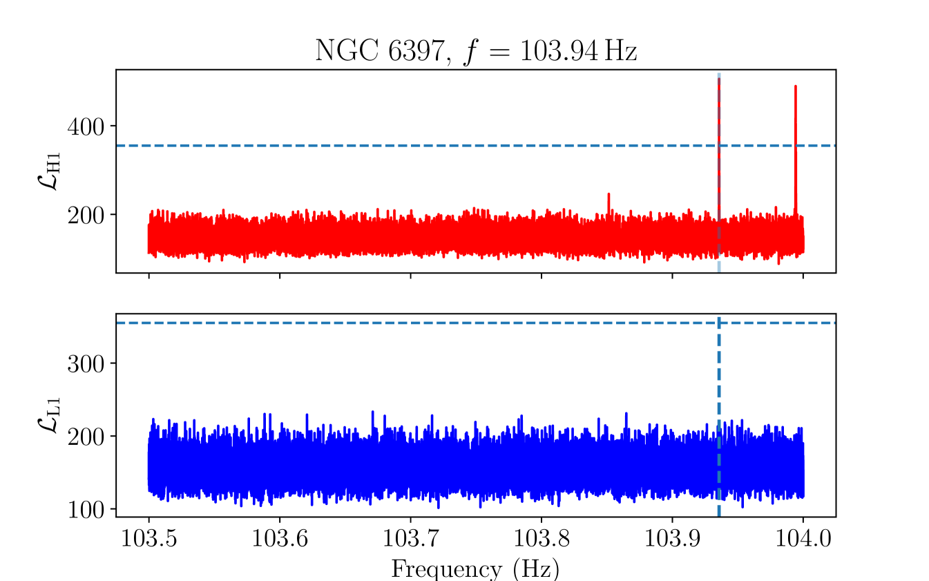
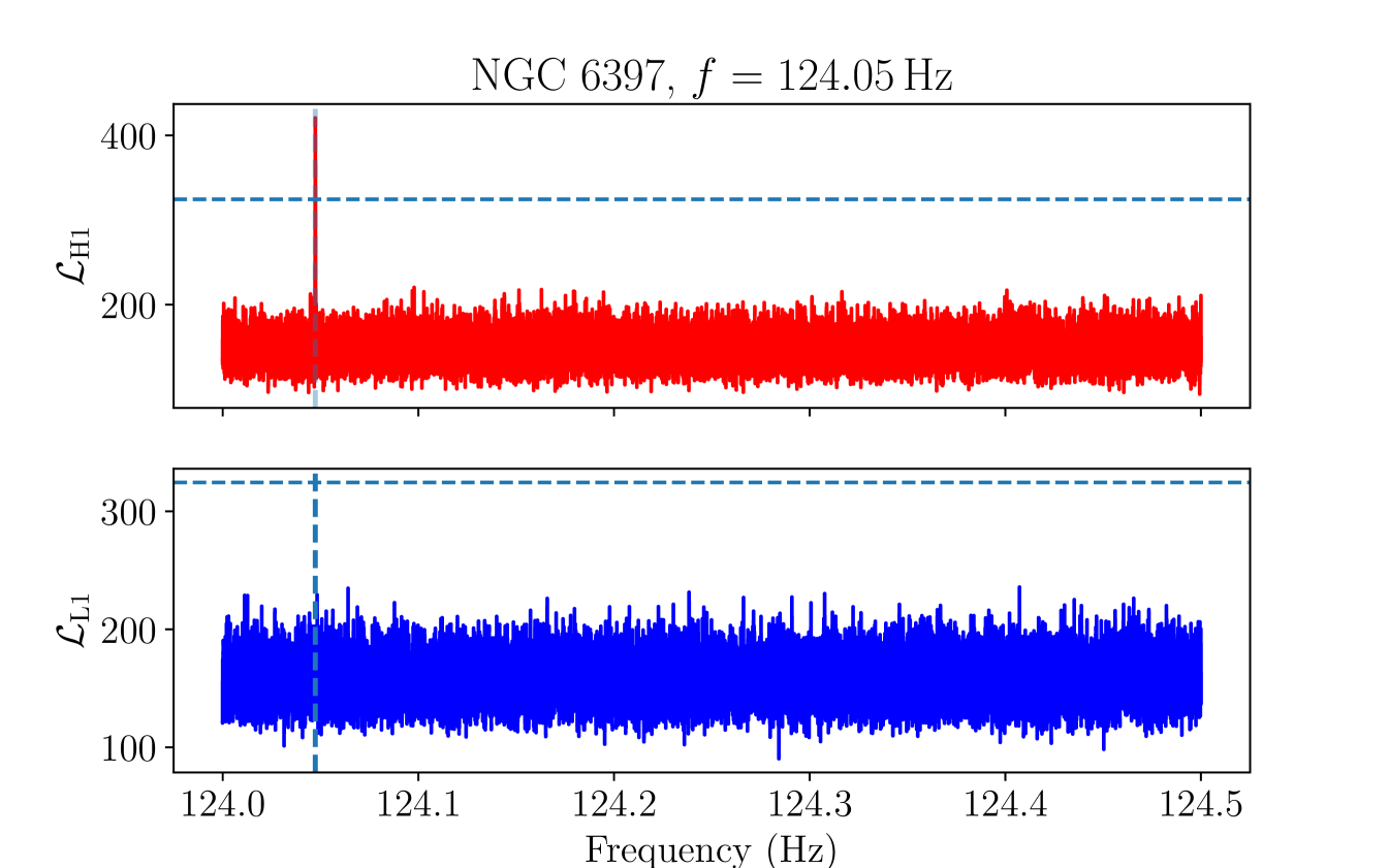
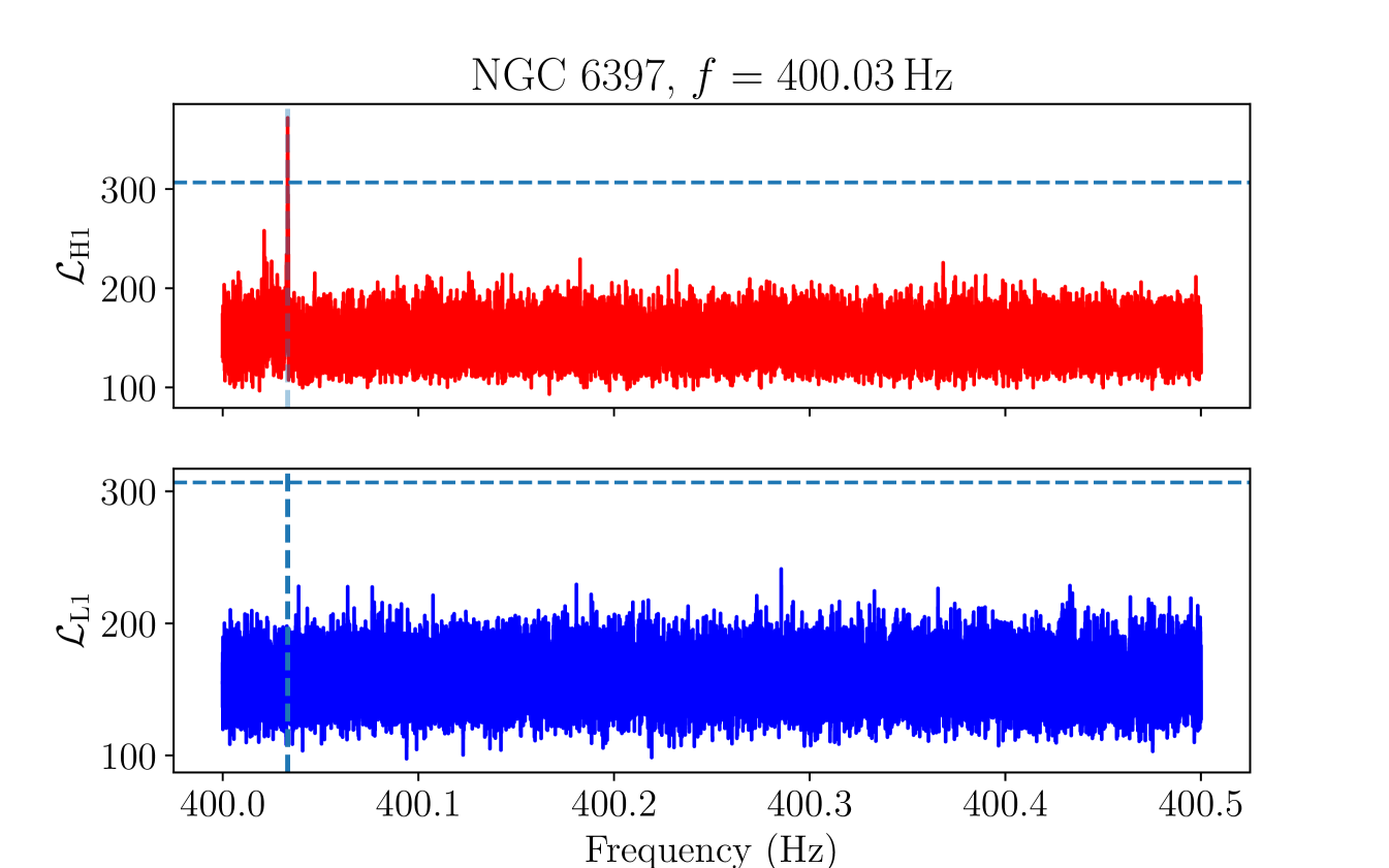
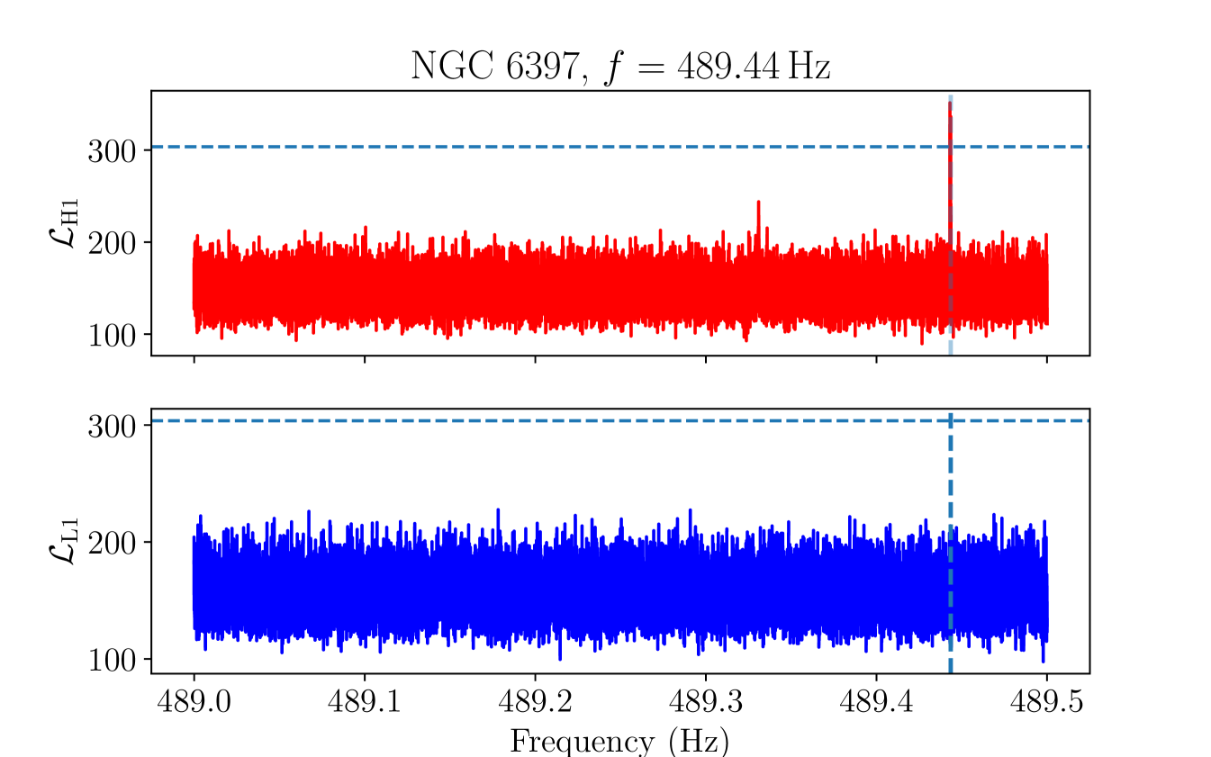
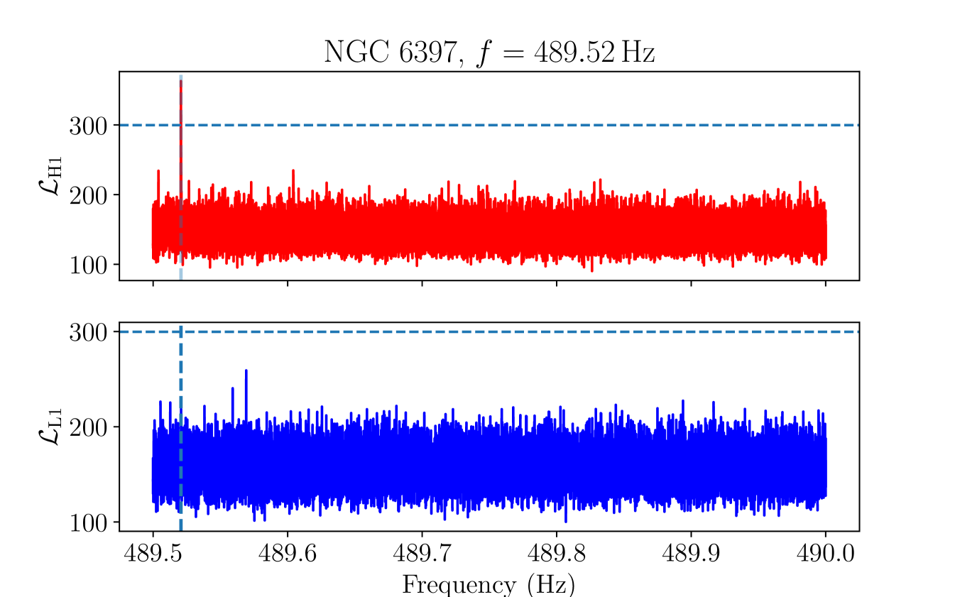
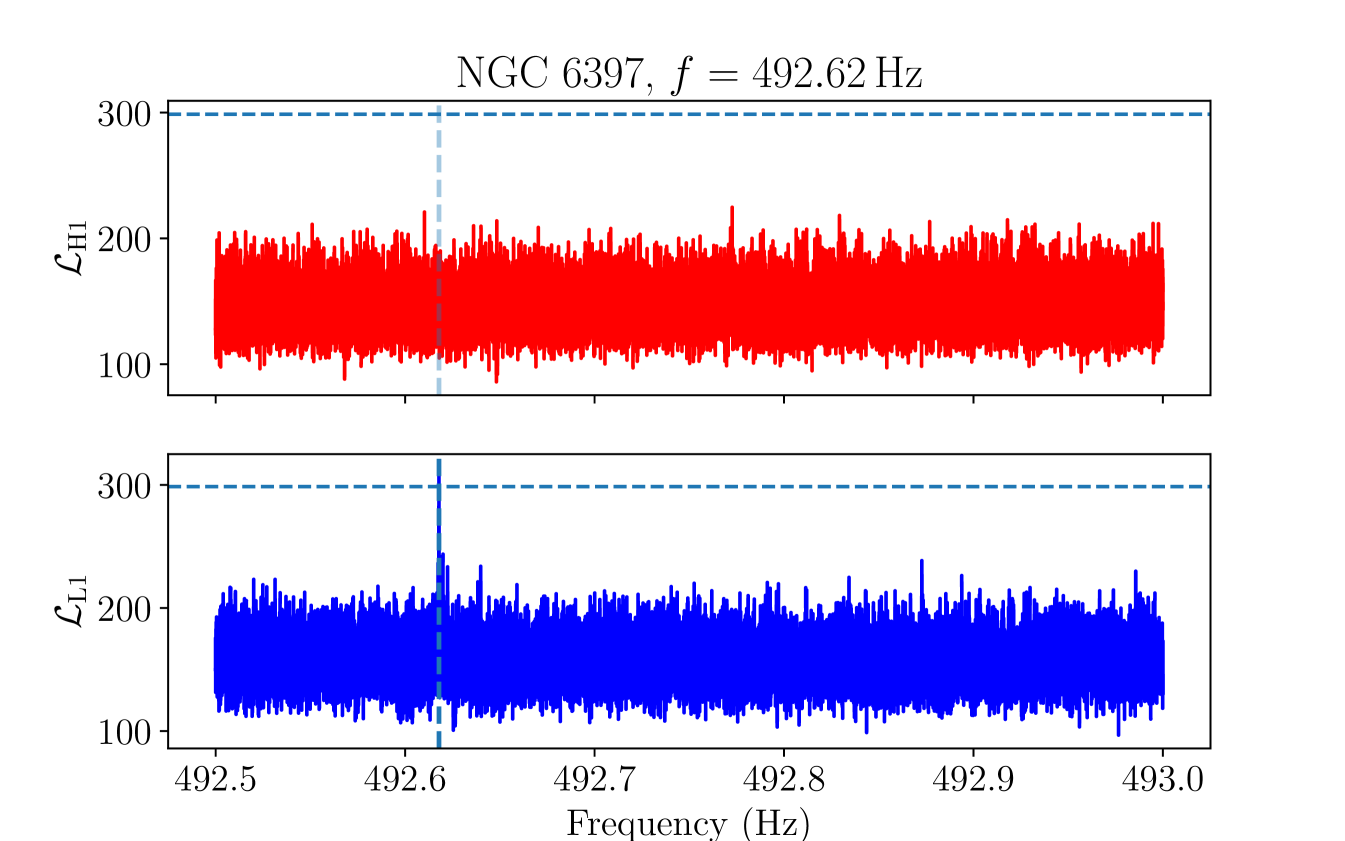
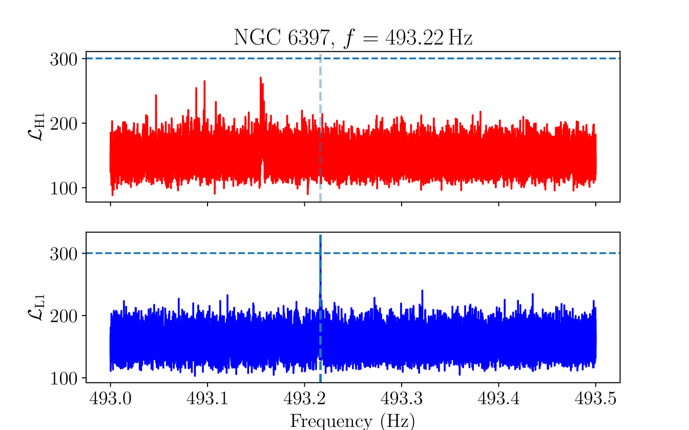
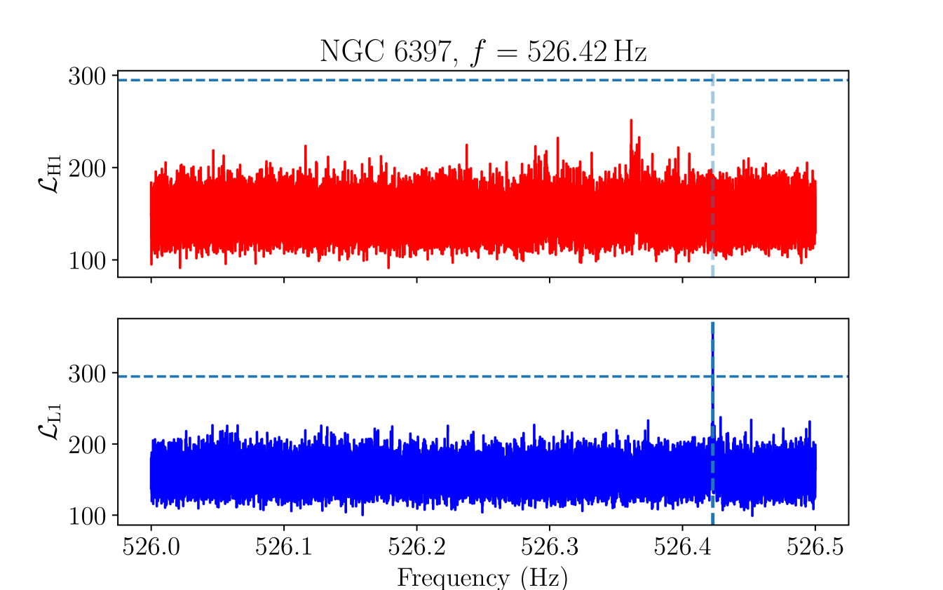
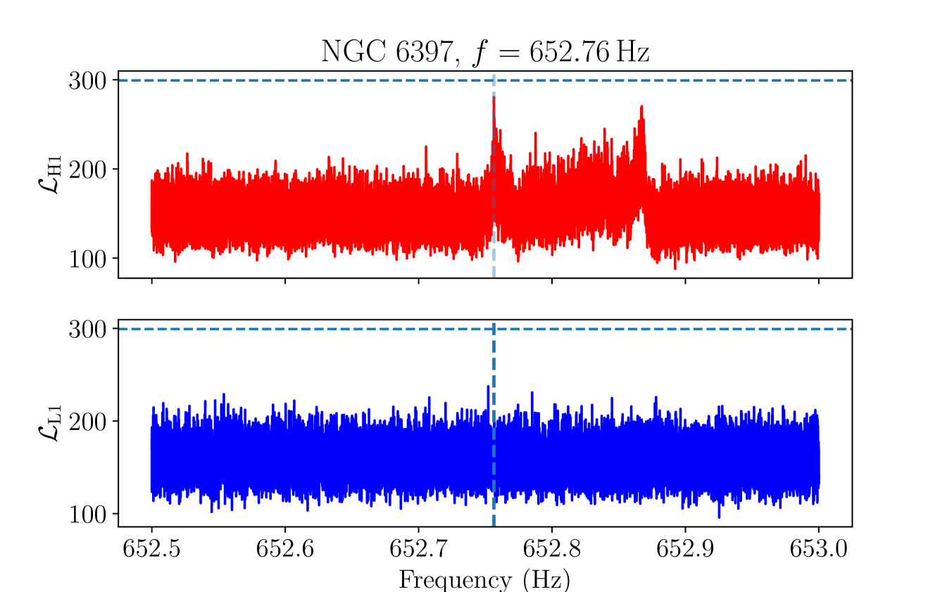
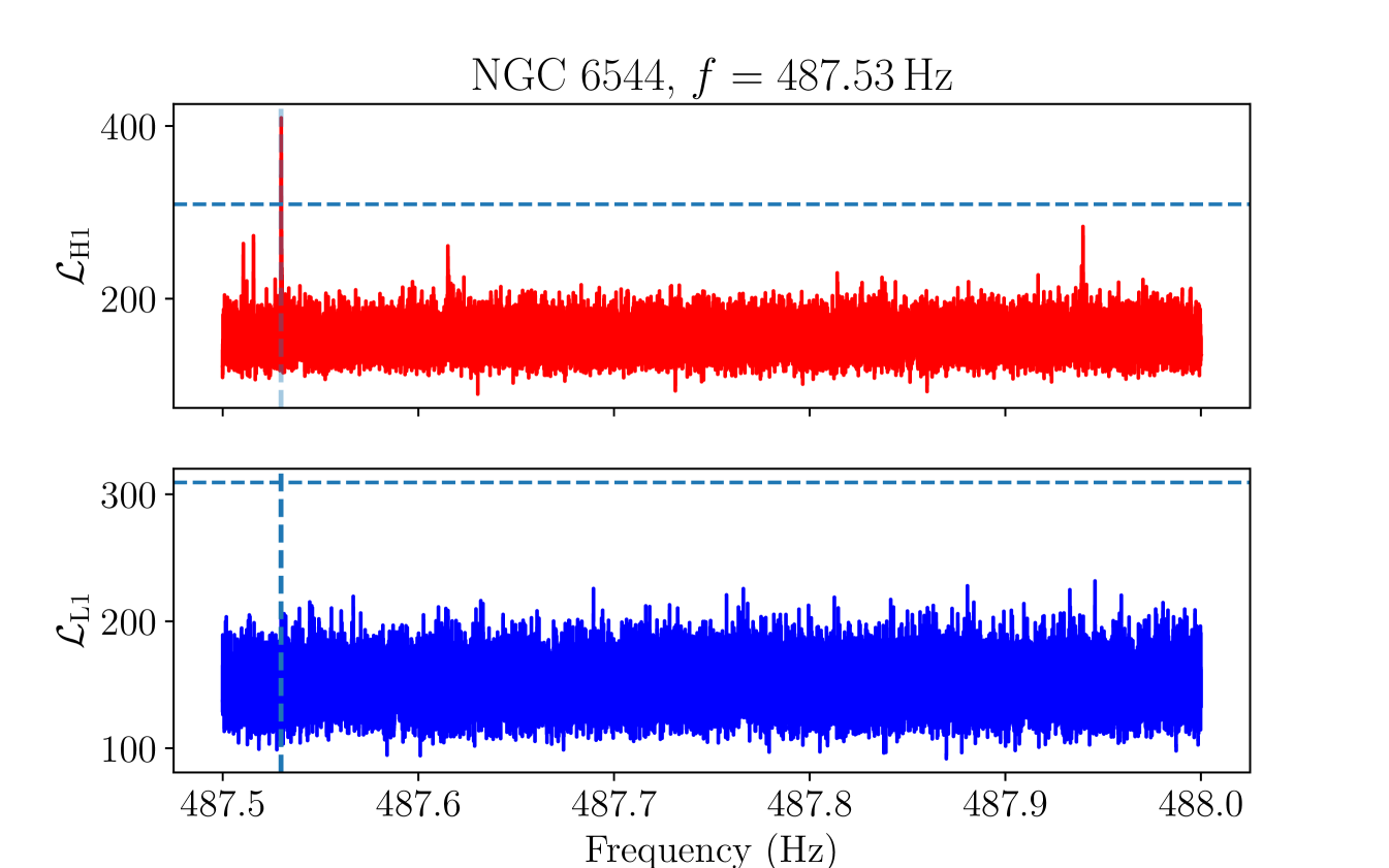
Appendix D Unknown lines
This appendix collects plots of the single-detector ASDs in the vicinity of the ten candidate groups which survive the cross-cluster veto (Section IV.3.1). The plots are displayed in Figure 10. Although all but one of these candidate groups are vetoed by the single-interferometer veto (Section IV.3.2), we present the single-detector ASDs for completeness. Seven of the ten candidate groups show a disturbance in one ASD within the Doppler modulation window of the candidate group.