Search for Lepton Flavor Violating Signals at the Future Electron-Proton Colliders
Abstract
The search for lepton flavor violation (LFV) is a powerful probe to look for new physics beyond the Standard Model. We explored the possibility of searches for LFV boson couplings to electron and muon pairs at the upcoming electron-proton colliders, namely the Large Hadron Electron Collider (LHeC) and the Future Circular lepton-hadron Collider (FCC-eh). We employed the study via a single muon plus an associated jet channel to search for the LFV signal. We used a multivariate technique to obtain an improved signal-background analysis. By using the condition on nonobservation of any significant deviation of the signal over the expected background, we provide an upper limit on the LFV boson coupling and corresponding branching ratio. We find that an upper limit of and can be set on BR() at 95% C.L. with one year run of LHeC and FCC-eh, respectively, if the LFV coupling is governed by vector or axial-vector coupling. For tensor or axial-tensor coupling, these limits can be improved to and for LHeC and FCC-eh machines, respectively. The projected numbers improve significantly over the existing limit of set by ATLAS.
I Introduction
The successful framework of the Standard Model (SM) of particle physics is equipped with the conservation of lepton flavors, although the observations of neutrino masses and mixing SNO:2002tuh ; Super-Kamiokande:1998kpq provides non-zero lepton flavor violation (LFV)111The phrase ‘lepton flavor violating’ is also abbreviated as LFV in this article. The exact meaning of the abbreviation should be clear from the context. via the loop. The amount of such violations is extremely small to be detected in an experiment. To date, no experimental measurement shows a piece of direct evidence in support of charged LFV Calibbi:2017uvl ; ParticleDataGroup:2022pth . However, the violation of the lepton flavor always remains a topic of interest in the particle physics community. Primarily because an experimental observation of establishing lepton flavor violation opens up a plethora of avenues of new physics beyond the Standard Model (BSM). For example, various neutrino mass models, such as Type-II, Type-III, and inverse seesaw models, which generate neutrino mass at the tree level, exhibit LFV scenarios. On the other hand, some models having neutrino mass generated radiatively, e.g. Zee-Babu model, Scotogenic models, etc., also show signatures for LFV Konetschny:1977bn ; Foot:1988aq ; Sun:2013kga ; Mohapatra:1980yp ; Hisano:1995nq ; Herrero-Garcia:2014usa ; Babu:1988ki ; Zee:1980ai ; Ma:2006km ; Rocha-Moran:2016enp ; Hundi:2022iva .
A series of experiments, both dedicated and general-purpose, have been performed at various levels to search for LFV in the charged leptons. None of which shows any significant evidence for it. This, in turn, sets upper limits to the LFV branching ratios (BRs) of the decays and LFV couplings of the decays of various particles. The MEG experiment sets an upper limit on BR() at MEG:2016leq , the SINDRUM experiment sets an upper limit on BR() at SINDRUM:1987nra , the BaBar experiment sets an upper limit on BR at and on BR at BaBar:2009hkt , the Belle experiment sets a limit on BR and BR Hayasaka:2010np at 90% C.L. at all the experiments.
Another series of bounds are given on the LFV decays of heavy neutral bosons. These types of bounds primarily come from the collider experiments because of their ability to produce on-shell heavy bosons. The LFV decays of such particles have been searched for at the Large Hadron Collider (LHC). The limits on the BRs of the Higgs boson in the , , and channels have been set to be no more than CMS:2016cvq , , and CMS:2017con , respectively at 95% C.L. by CMS collaboration at the LHC. On the other hand, the searches for lepton flavor violating decays (LFVZD) date back to the era of the Large Electron-Positron (LEP) collider, where the neutral boson could be produced copiously. The LFV decays of neutral boson have been measured in , , and channels in the LEP by OPAL, and DELPHI collaborations OPAL:1995grn ; DELPHI:1996iox . However, the recent searches of LFVZD in the channel at the LHC by the ATLAS collaboration supersedes the previous bound LEP.
Many in-depth studies, both theoretical and experimental, of various LFV signals have been conducted in the context of lepton and hadron colliders. In the Hadro-Electron Ring Accelerator (HERA), LFV signals were looked at by H1 and ZEUS collaboration in the context of leptoquark searchesZEUS:1996bbn ; H1:1999dil ; ZEUS:2002dnh ; ZEUS:2005nsy ; H1:2007dum ; H1:2011rlk . The potential of electron-proton colliders like the Future Circular Collider (FCC-eh)FCC:2018byv and the Large Hadron electron Collider (LHeC)LHeCStudyGroup:2012zhm ; Bruening:2013bga ; LHeC:2020van , however, has not been covered fully in any of the literature that has been published thus far. Among these, the LHeC stands out owing to its capacity to function concurrently with the HL-LHC, made possible by the establishment of the energy recovery linac especially for the electron beamLHeC:2020van . Although the major objective of electron-proton colliders is to give high-precision data that enables precise determination of the parton distribution functions of a proton, their special benefits over pp colliders in identifying rare BSM events have not been adequately recognized. The use of an electron beam can curb underlying events, pile-ups, or QCD backgrounds in particular. When examining rare BSM events, which may easily be wiped out by the overwhelming presence of more than 150 pileups at the HL-LHC, the insignificant pileup environment of LHeC (FCC-eh) is roughly 0.1 (1) pile-up collisions per event proves to be quite helpful. One also can anticipate strong background control for electron-proton colliders by separating charged-current (CC) and neutral-current (NC) processes, as well as determining the forward direction. Therefore, the study of LFV could be explored in more detail in the upcoming electron-positron colliders.
The projections for such LFV decays have also been studied in the future electron-positron colliders Etesami:2021hex ; Calibbi:2021pyh ; Altmannshofer:2023tsa ; Dev:2017ftk . Similar studies have also been performed in the future electron-proton colliders Alan:2001cf ; Gonderinger:2010yn ; Accardi:2012qut ; Cirigliano:2021img ; AbdulKhalek:2021gbh ; AbdulKhalek:2022hcn ; Jueid:2023fgo . However, these studies primarily focused on the electron-tau LFV scenarios. In this work, we investigate the discovery potential of LFV in future electron-proton colliders, namely the Large Hadron Electron Collider (LHeC) and Future Circular lepton-hadron Collider (FCC-eh). We have primarily looked at the possibility of measuring BR() at these upcoming colliders. For this, we employed a search strategy via channels, where a single is produced due to the LFV coupling with the boson. This channel can provide us good sensitivity depending on the type of coupling, namely vector, axial-vector, tensor, or axial-tensor, with the boson. Our study suggests that at least a comparable (to the LHC) result can be obtained in the LHeC, and an improved result can be expected at the FCC-eh machine.
The outline of this article is as follows. In Section II, we briefly discuss the generic Lagrangian providing LFV coupling of the boson. We describe our analysis strategy in Section II.1. We then discuss the methods and multivariate analysis in Section II.2. We present our result in Section III. After that, we summarize our findings in Section IV.
II Prospect of LFV boson coupling at electron-proton collider
We study the LFVZD in a model-independent way. For this, we consider the following general-purpose BSM Lagrangian.
| (1) |
where represents the generation lepton and ’s are the coupling constants of and pair with the boson. The subscript of essentially indicates the Lorentz structure, namely vector (), axial-vector (), tensor (), or axial-tensor (), of the couplings with the boson. Equation (1) represents a general and model-independent Lagrangian. This Lagrangian should not be identified as an ultraviolet complete model. In the popular BSM models, these types of interaction are usually generated when the particles with non-diagonal flavor coupling to the lepton sector run in the loop Illana:2000ic ; DeRomeri:2016gum . In the flavor conserving models, the flavor off-diagonal couplings of the boson with the leptons are absent in the tree-level Lagrangian, thereby avoiding the ultraviolet divergences via the loops. However, they necessarily impose relations between the different couplings.
In terms of these couplings, the branching ratio of boson to pair becomes
| (2) |
where and , respectively, are the SM vector and axial-vector couplings of the boson with the charged leptons. In Eq. (2), we assumed the total decay width of the boson to be that of the SM since the BSM contributions to the total decay width is negligible. The upper limit on the branching ratio of LFVZD can be translated to the couplings on the Lagrangian in Eq. (1). In Table 1, we tabulate the current upper limits on various LFV boson branching ratios and the derived upper limit on the coupling constant, considering a single coupling at a time. The limit on the vector and axial-vector provides the same BRs, and, therefore, they have the same limit. Likewise, the tensor and axial-tensor coupling constants have the same derived upper limits.
| Experiment | BR | = | = | |
|---|---|---|---|---|
| ATLAS ATLAS:2022uhq | GeV-1 | |||
| ATLAS ATLAS:2021bdj | GeV-1 | |||
| ATLAS ATLAS:2021bdj | GeV-1 |
II.1 Signals and Backgrounds
In order to study the LFV scenario in an electron-proton collider, we consider the process
| (3) |
The LFV couplings introduced in the Lagrangian in Eq. (2) would induce such a process. In any electron-proton collider, the production of a single muon without any source of missing energy is unlikely in the SM because of the conservation of the lepton number of each generation. Therefore, this provides an interesting channel to search for lepton flavor violations. If no signal for such violation is observed in the collider, one may put a constraint on the LFV couplings introduced in Eq. (1). We then can use this bound on LFV couplings to provide an upper limit on the branching ratios of the LFVZD. In this work, we will be considering one type of coupling out of the , , , or , that is to say, one of vector, axial-vector, tensor, or axial-tensor operators at a time in our analysis. We have differed the scope of the study containing more than one operator in a separate work.
We have considered the Large Hadron Electron collider (LHeC) and the Future Circular lepton-hadron Collider (FCC-eh) for the searches for the above signal. Each machine has been proposed to run in two phases. We label these phases as ‘LHeC1’, ‘LHeC2’, ‘FCC-eh1’, and ‘FCC-eh2’ for further reference. We also list the most important specifications of these machines in Table 2.
| LHeC1LHeCStudyGroup:2012zhm | LHeC2Bruening:2013bga | FCC-eh1LHeC:2020van | FCC-eh2FCC:2018byv | |
|---|---|---|---|---|
| Electron energy [GeV] | 30 | 50 | 60 | 60 |
| Proton energy [GeV] | 7000 | 7000 | 20000 | 50000 |
| Luminosity [nb-1s-1] | 5 | 9 | 8 | 15 |
| Integrated Luminosity (1 year run) [fb-1] | 50 | 90 | 80 | 150 |
In - collision, the signal process comes up due to the flavor changing vertex of via a -channel exchange of boson. This particular channel is not present in the SM. However, some other SM processes can give rise to the final state as the signal. The following SM processes are considered to be potential backgrounds for our signal.
| Photoproduction: | |||
|---|---|---|---|
| mu: | |||
| e-mu: | |||
| mu-mu: |
-
•
Photoproduction: The primary background comes from photoproduction Bauer:1977iq ; Chwastowski:2003aw ; ZEUS:2005nsy ; H1:2011rlk , wherein direct or resolved photons from the electron beam interact with the proton beam. The hadronic final states can give rise to muons from the (semi)leptonic decays of heavy or mesons.
-
•
mu: Another important background comes from the production of a boson and a jet along with an invisible neutrino. The boson can then decay into a muon and a neutrino. This background contains a single muon and has the same visible final states as that of the signal. However, the large missing energy from the invisible neutrinos makes the background reduction easier.
-
•
e-mu: The third main background primarily comes from the production of an electron, a jet, and a boson. The subsequent decay of boson to muon channel gives a similar final state as the signal if the electron in the final state gets missed. The source of missing energy makes the background reduction easier.
-
•
mu-mu: The fourth background is similar to the first one with the exception of the production of boson along with the jet and MET. The decay of to two muons and one of them being missed makes its final state identical to the signal.
We further note that the same event topology in the backgrounds also appears when the vector bosons decay to and the then decays leptonically. We have taken care of this aspect in the background event generation.
For further signal-background analysis, we have implemented the new Lagrangian described by Eq. (1) in Feynrules Alloul:2013bka to obtain the Universal Feynman Object (UFO) Degrande:2011ua files. Then, the UFO model is used to generate the signal events for the scattering process. The signal and background events at the parton-level have been generated using MadGraph5@aMCNLO (v3.4.2) Alwall:2011uj at the lowest order. At the parton-level event generation, we have imposed GeV, GeV, , cuts. These parton-level events have then been showered using Pythia8Sjostrand:2014zea and stored in HepMC2Buckley:2019xhk formatted files. The photoproduction background has been generated using Pythia8 and stored in HepMC2 format. These events have then been passed onto DelphesdeFavereau:2013fsa for detector simulation. For the efficiencies of different objects, we have used the default card for LHeC and FCC-eh provided in Delphes (version 3.5.0). We then used fastjet3Cacciari:2011ma to form jets from the Delphes generated Particle Flow (PF) candidates.
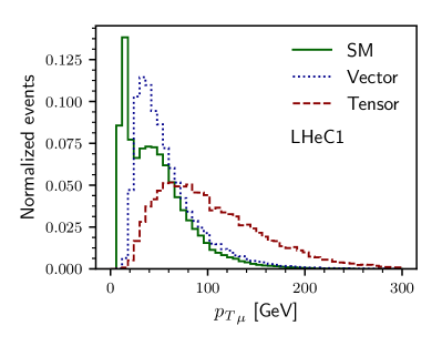
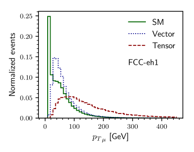
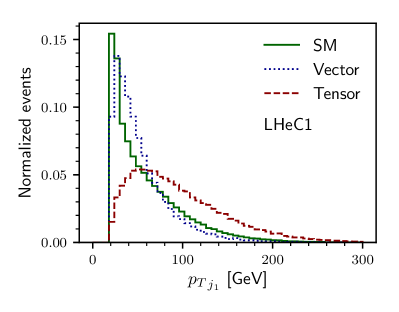
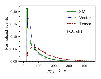
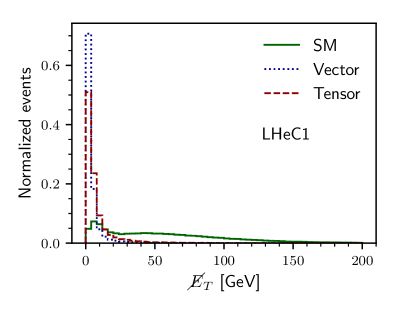
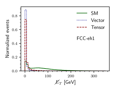
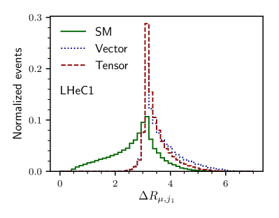
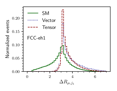
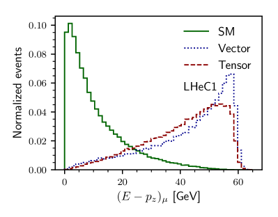
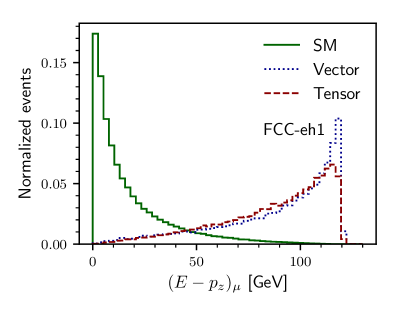
The key to any signal-background analysis is to put some valuable cuts on some variables which can give us a signal-favored region with more signals and fewer backgrounds. To know those good variables in the signal and backgrounds plane, we illustrate, in Figs. 1 and 2, the normalized distributions of some important variables. In Fig. 1, we show the and distribution for the three different backgrounds and the signal with non-zero vector and non-zero tensor coupling. The variable distribution for the signal with non-zero axial-vector and non-zero axial-vector couplings are similar very much similar to their non-axial counterparts and, therefore, are not shown. Figure 1(a) is for the distribution of for LHeC1 and Fig. 1(b) is for FCC-eh1 machine. In the bottom row of Fig. 1, we show the normalized distribution of transverse momentum of the leading jet () for the signal and backgrounds having the same machine energies. Because of the momentum dependence factors in tensor couplings, the distributions of and have long tails for higher compared to the vector coupling scenario. Similarly, in the top row of Fig. 2, we show the distribution of missing transverse energy for both LHeC1 (Fig. 2(a)) and FCC-eh1 (Fig. 2(b)). In the second row, we illustrate the distribution of between the muon and the leading jet for LHeC1 (Figs. 2(c)) and for FCC-eh1 (Fig. 2(d)).
In electron-proton collider, another useful variable for the signal, in which no sources of missing energy are expected, is variableZEUS:2005nsy ; H1:2011rlk , defined as the sum of the differences of energies and -component of the momenta of all final state visible particles. The -axis is defined in the direction of the proton beam, and, in the absence of invisible particles in the final state, should be equal to twice the electron beam energy (). Since the signal is a -channel process, is expected to be closer to , and is expected to be close to zero. In Fig. 3, we show the distribution of for both LHeC1 (Fig. 3(a)) and FCC-eh1 (Fig. 3(b)). From the distribution of and , one can easily guess that these are good variables for reducing the SM backgrounds over signal with both types of couplings and in both colliders. Further inspection of the other variable might reveal more interesting signal region. Instead of manually inspecting on all possible event variables, we do the signal and background separation with the help of multivariate analysis. To gain the machine learning advantage in the computation time, we provide a cut of before sending the variables to the multivariate analysis tool. Although the also looks to have significantly different distributions between signal and background, we did not put any cut on it before the multivariate analysis. It is because the preselection cuts on the missing transverse energy reduce a significant amount of backgrounds.
Keeping these in mind, we have imposed the following preselection cuts for the signal and the backgrounds.
| (4) |
After putting the preselection cuts, the cross sections for our signal and backgrounds for all types of coupling for different machine energies are listed in Table. 3.
| LHeC1 | LHeC2 | FCC-eh1 | FCC-eh2 | |
| Cross-section [fb] | ||||
| BKG Photoproduction | 16.28 | 23.41 | 93.93 | 169.80 |
| BKG mu | 4.58 | 9.60 | 20.20 | 31.40 |
| BKG e-mu | 6.88 | 14.40 | 29.30 | 43.50 |
| BKG mu-mu | 0.57 | 0.83 | 1.47 | 2.13 |
| Vector | 0.07 | 0.10 | 0.17 | 0.25 |
| Axial Vector | 0.07 | 0.10 | 0.17 | 0.25 |
| Tensor | 0.36 | 0.65 | 1.27 | 1.95 |
| Axial Tensor | 0.36 | 0.65 | 1.27 | 1.95 |
II.2 Multivariate analysis
After applying the aforementioned cuts on the observables for signal and background events, we move on to investigate potential improvements in separating signal from the background using some established machine learning methods, such as Gradient Boosted Decision Trees Roe:2004na . In comparison to rectangular cut-based analysis, these techniques have been widely employed in the literature recently and have been found to offer a superior separation of the signal from the background. The key objective here is to build a one-dimensional observable after appropriately combining the important observables that may effectively distinguish our signals from the background. We have used XGBoost Chen:2016btl toolkit for gradient boosting in this analysis.
| Variable | Definition |
|---|---|
| Transverse momentum of the leading muon | |
| Transverse momentum of the leading jet | |
| Missing transverse energy | |
| No of muons in the event | |
| No of jets in the event | |
| Invariant mass of the leading muon and leading jet | |
| The cluster transverse mass Dey:2020tfq | |
| Transverse mass | |
| Scalar sum of of all the final state particles | |
| between leading muon and leading jet | |
| between leading muon and missing energy | |
| between leading jet and missing energy | |
| between leading muon and leading jet | |
| Difference between energy and longitudinal momentum of leading muon | |
| Difference between energy and longitudinal momentum of leading jet |
For further analysis, a total of input variables, called feature variables, have been used for the training and validation of our data sample. The variable, along with their definition and description, is provided in Table 4. With a maximum depth of 3 and a learning rate , we have taken about 1000-3000 estimators for the gradient-boosted decision tree technique of separation. We have used 70% of the whole dataset for training purposes and 30% for validation in both XGBoost analyses. Overtraining of the data sample is one potential drawback of these strategies. In cases of overtraining, the test sample cannot match the training sample’s incredibly high accuracy. With our selection of parameters, we have specifically verified that the algorithm is not overtrained.
III Result and Discussion
As mentioned previously, we have considered a single coupling at a time in order to find out the upper limit on the BR of decay. In the last section, we noticed that our vector-only coupling and axial-vector-only coupling are not noticeably different from each other. The same is true for tensor-only and axial-tensor-only couplings. Therefore, in the following subsections, we plan to discuss the result from the vector-only coupling scenario and axial-vector-only scenarios. In the subsection after that, we plan to discuss the tensor-only and axial-tensor-only coupling scenarios.
III.1 Vector and axial-vector coupling
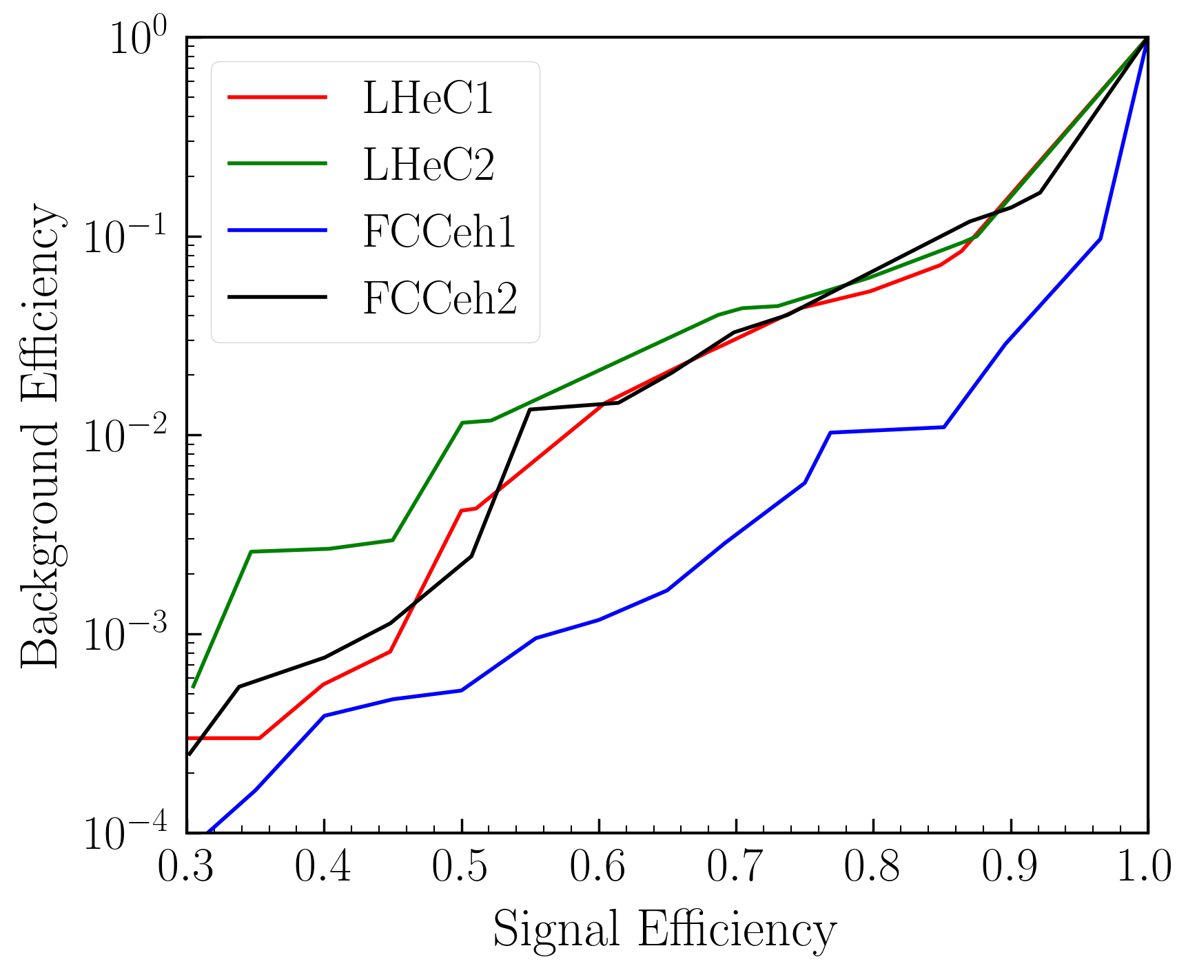
For the discussion in this subsection, we have chosen only to be non-zero. We first show, in Fig. 4(a), the performance of the BDT network through the Receiver Operating Characteristic (ROC) curve. The good performance of the network is evident from the figure. The background acceptance is below 0.01 with 50% signal efficiency. This high performance is because most of the backgrounds contain neutrinos, a source of missing energy, in contrast to the signal, where there is no source of missing energy. The network returns the BDT classifier variable, which can then, in principle, be used to set a cut and calculate the signal significance. We have shown these signal significances as a function of signal efficiencies.
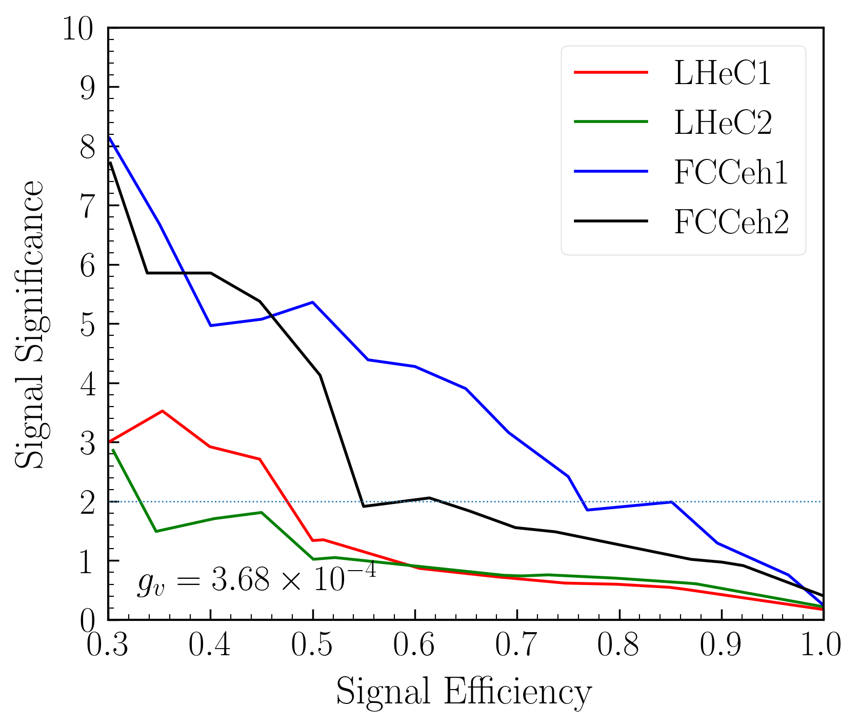
For given signal efficiency and background efficiency , the signal efficiencies are calculated as
| (5) |
where are the cross section for signal (backgrounds), and represents the integrated luminosity. The Variation of signal significance as a function of signal efficiency is shown in Fig. 4(b) for all the four machine energies as described in Table 2. A feature of the curves shows that the signal significance is the best in the region 30% to 50% signal efficiencies. The background efficiencies in this region are actually substantially small which varies between to . The region below 30% of signal significance suffered from a very low number of backgrounds (sometimes zero). As a result, this area is not reliable as there is a mismatch between the train and test samples.
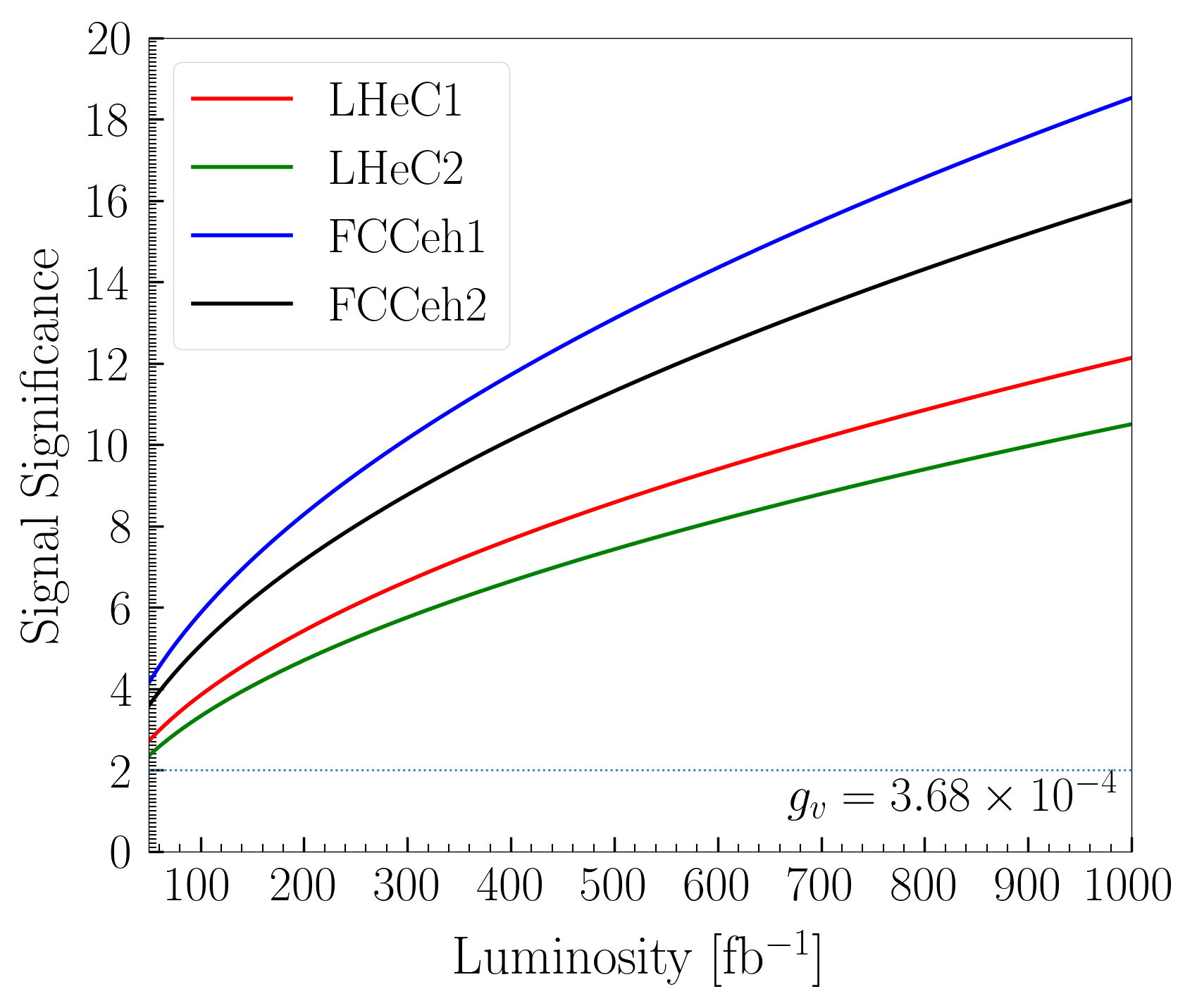
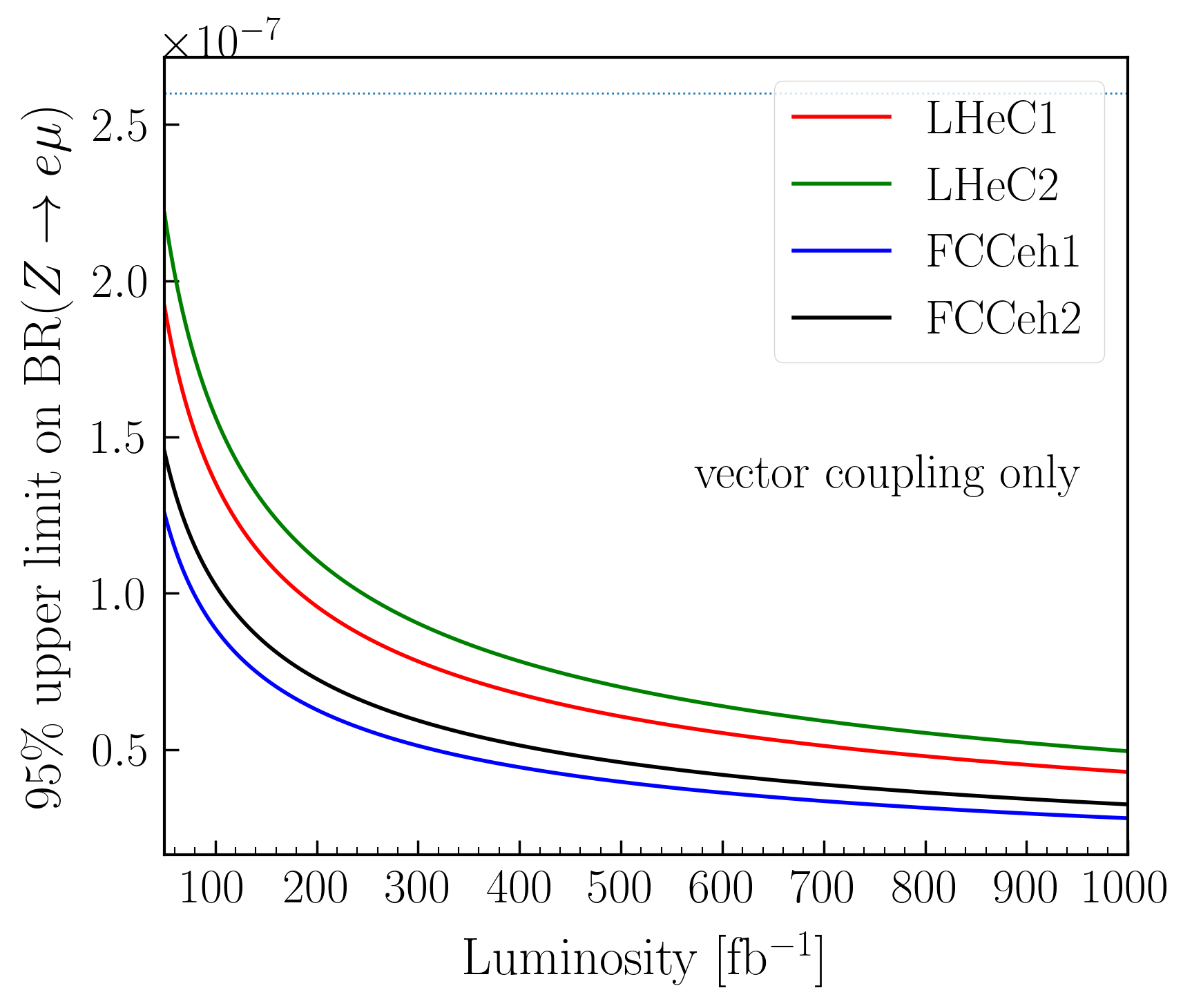
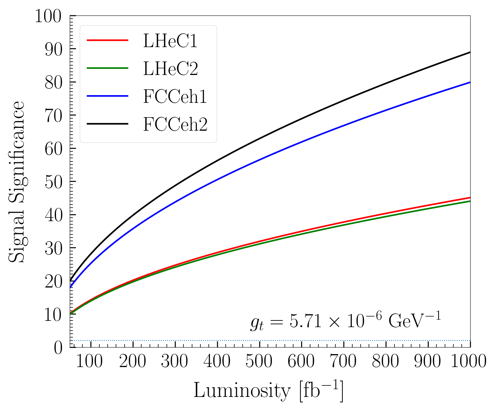
We then choose our working points to be in the range of from 0.3 to 0.5, depending on maximum achievable signal significance. The four different machine energies, therefore, have different working points. We also ensured that there was a good agreement in the distribution between the test and train samples at those working points. The variation of signal significance as a function of integrated luminosity has been shown in Fig. 5(a) for four different colliders. One can observe that the signal significance is distinctively better ( times better) in FCC-eh1 and FCC-eh2 compared to all LHeC energies. Furthermore, for a given luminosity, the signal significance varies as the square of the coupling constant . Now, we can, in principle, put an upper limit on the coupling constant at a signal significance. That is, to say, the value of at which 2 signal significance is achieved. These limits on can then be translated into the limit on the LFV boson BRs by using Eq. 2. We plot, in Fig. 5(b), the upper limit on BR() at 95% C.L. as a function of luminosity for four different machines. In Fig. 5(b), the horizontal line represents the current bound by the ATLAS collaborationATLAS:2022uhq , which is achievable below 50 fb-1 in all the future electron-proton colliders.
III.2 Tensor and axial-tensor coupling
Similar to the previous subsection, we then performed an analysis with the tensor LFV coupling. In this case, we have only the tensor coupling to be non-zero at . We first show the ROC curves for four different machines in Fig. 6(a).
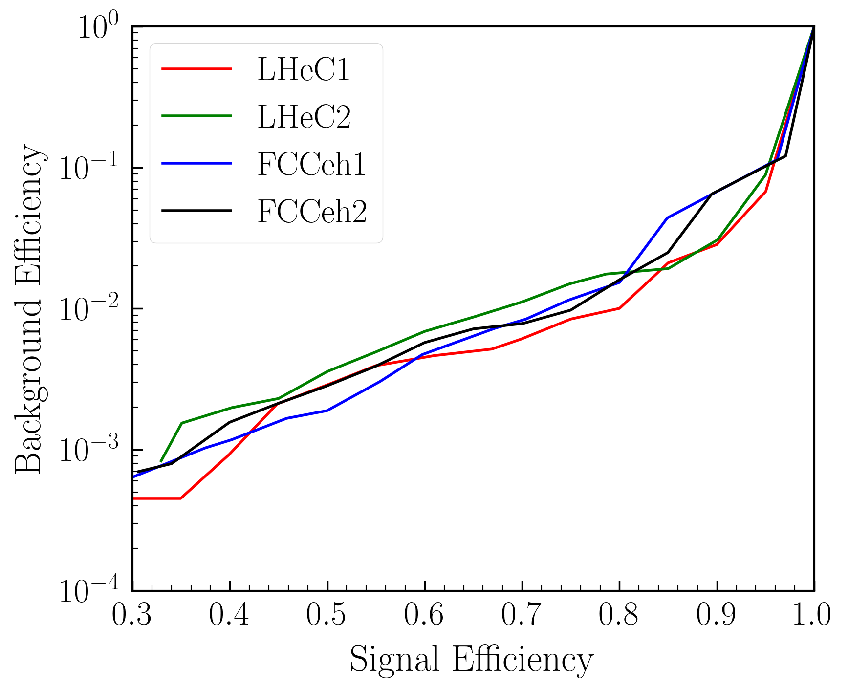
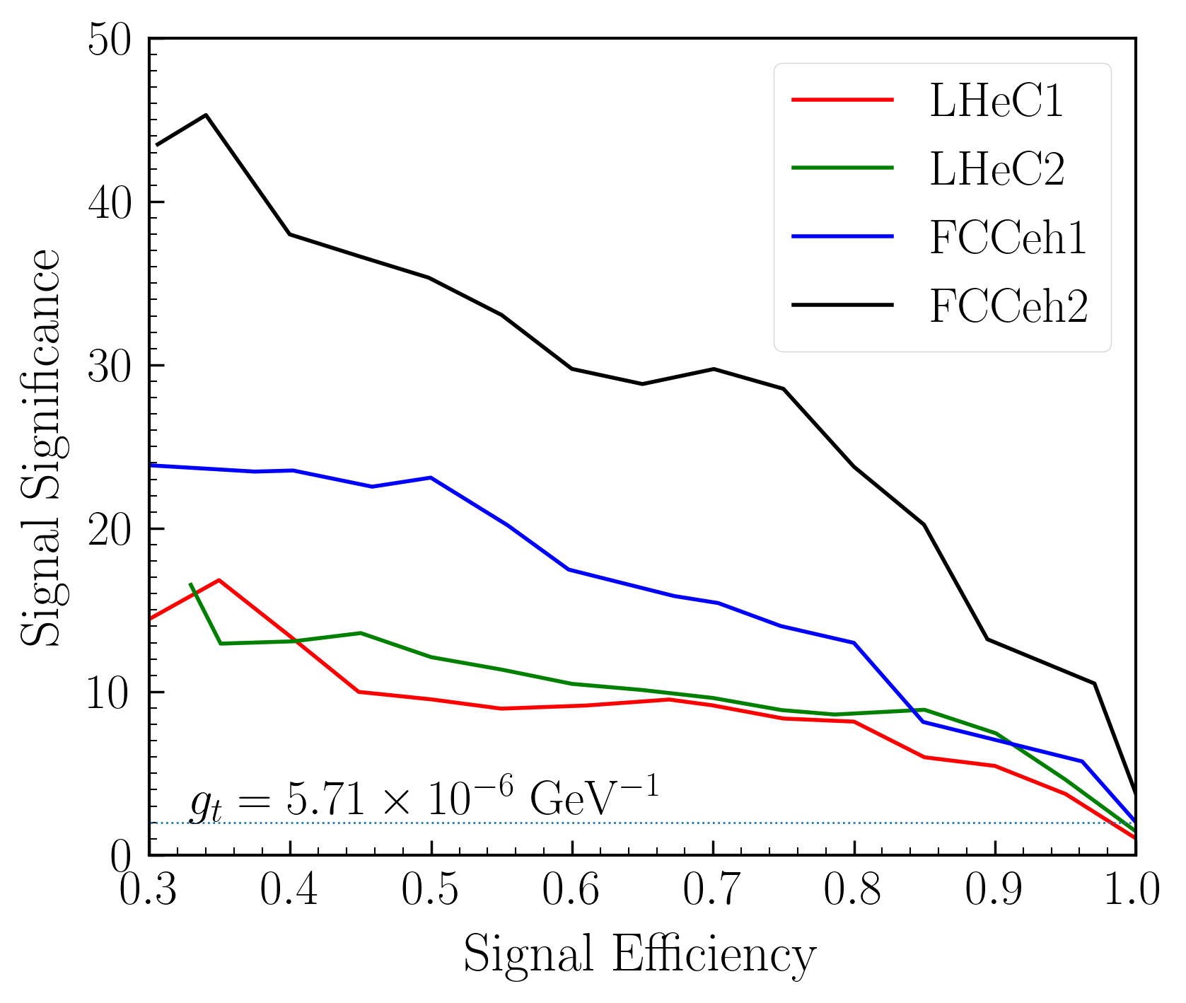
The ROC curves actually feature a very good separation between the signal and the backgrounds. In all the machine energies, the background acceptance rate is between to signal significances between 30% to 70%. Signal significance as a function of signal efficiency has been plotted in Fig. 6(b). We can see that, in the case of tensor-only coupling, FCC-eh runs can provide better (approximately a factor of 1.2 - 3.0) significance than LHeC runs. Although a quick comparison between Fig. 4(b) and Fig. 6(b) may indicate that the tensor-only coupling provides better signal significances, we note that they should not be compared as the coupling values, at this point, are arbitrary and they are for demonstration only.
We then choose our working points to be in the range of , from 0.3 to 0.5, which yields the maximum signal significance that we can achieve. We show in Fig. 7(a) the variation of signal significance as a function of luminosity. To affirm no overtraining, we ensure good agreements in the distribution between the test and train samples in our chosen . The signal significances are above 2 even with 50 fb-1 in the case of LHeC runs and are well above 2 in the case of FCC-eh runs.
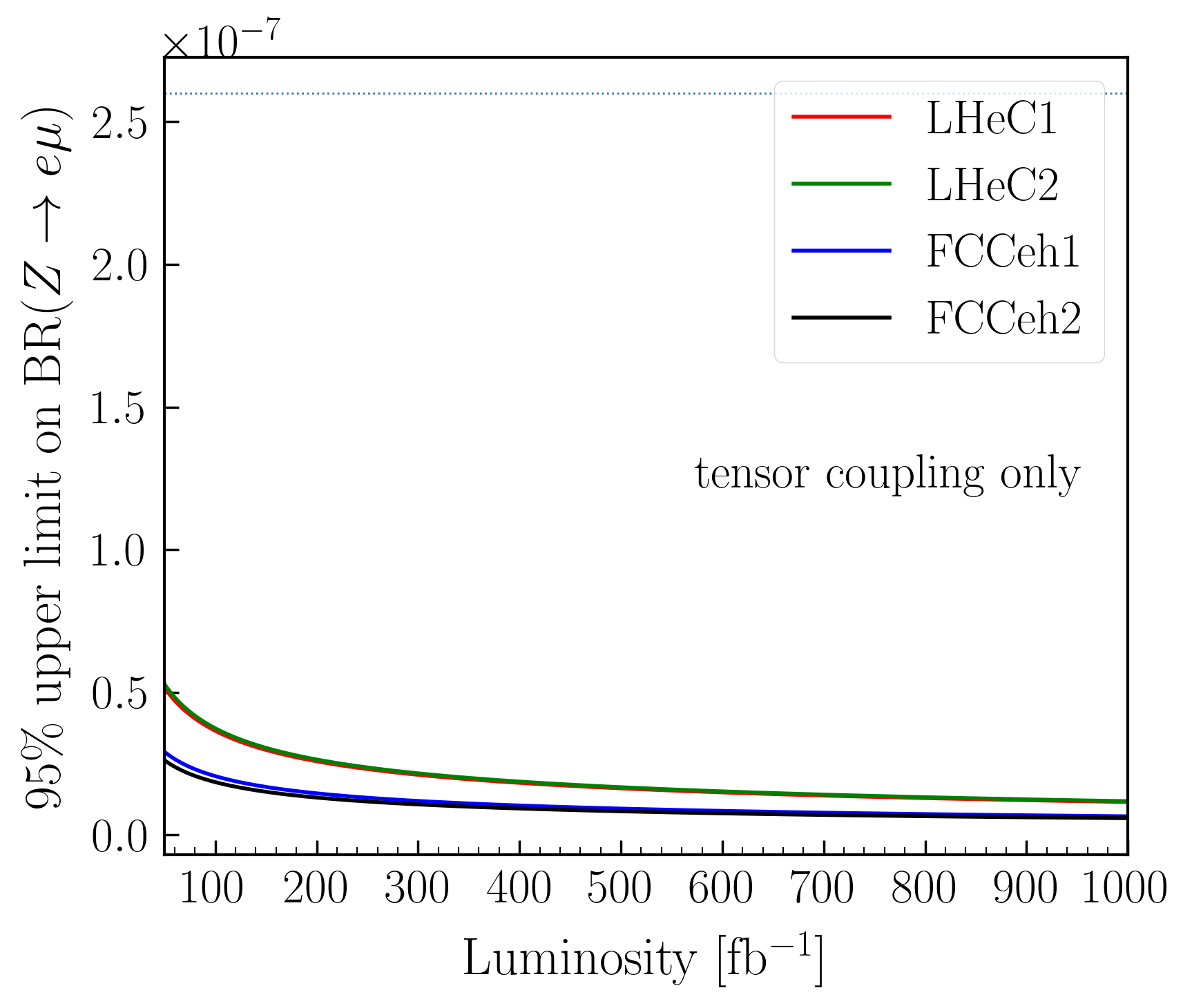
The projected upper limit on BR() as a function of integrated luminosity at the best value with highest significance, has been plotted in Fig. 7(b). In the case of tensor-only coupling, one can see that the current bound on BR() at 95% C.L. can easily be achieved with less than 50 fb-1 integrated luminosity in all four machine energies.
III.3 Bounds on LFV branching ratio
We now put together the results from the last two subsections by providing projected bounds on BR() for four different machine energies. As we mentioned previously, we consider only one effective coupling at a time. These projected bounds on the branching ratio and the effective coupling are shown in Tables 5 and 6. We have considered a one-year runtime of each machine and the integrated luminosity as provided in Table 2.
| Projected upper bound @95% CL on BR() and couplings | ||||
| LHeC1 | LHeC2 | |||
| Coupling Type | BR() | BR() | ||
| Vector | ||||
| Axial Vector | ||||
| Tensor | GeV-1 | GeV-1 | ||
| Axial Tensor | GeV-1 | GeV-1 | ||
| Current upper bound @95% CL on BR() from ATLAS is | ||||
As was hinted at by the discussions in the previous two subsections, we note that the future electron-proton collider has the potential to provide a stronger upper bound. As mentioned in Table 2, if we look in the LHeC case, for run 1, an integrated luminosity around fb-1 can be achieved, and for run 2, it can be fb-1 after collecting one year of data. Considering that we can marginally improve the limit on BR() compared to the current bound provided by the ATLAS collaborationATLAS:2022uhq for the case of vector-only and axial-vector-only coupling. On the other hand, if the new physics LFV couplings are governed by tensor or axial-tensor coupling, the bound on BR() can be times stronger than the current upper limit. Overall, there is a scope for improvement in the current bounds at both runs of the LHeC machine. These numbers are calculated assuming that the run is for one year only. With more than one year run, there is further scope for improvement.
| Projected upper bound @95% CL on BR() and couplings | ||||
| FCC-eh1 | FCC-eh2 | |||
| Coupling Type | BR() | BR() | ||
| Vector | ||||
| Axial Vector | ||||
| Tensor | GeV-1 | GeV-1 | ||
| Axial Tensor | GeV-1 | GeV-1 | ||
| Current upper bound @95% CL on BR() from ATLAS is | ||||
Let us look at the FCC-eh case now. In that case, with the run-1, we can get an integrated luminosity of fb-1 and for run-2, it can be fb -1 after collecting all data for one year. So, if one only focuses on the luminosity after one year run for FCC-eh run 1, the improvement on the BR() can be times stronger than the existing bound set by ATLAS for the case of vector-only and axial-vector-only coupling. Whereas, for tensor-only or axial-tensor-only coupling, the improvement can be more than a factor of . On the other hand, a more remarkable improvement can be shown if we take a look at the FCC-eh run-2 case. In that case, after the collection of one-year data, the bound can be times stronger compared to the existing bound. For a run of more than one year, these projected bounds are expected to become stronger.
IV Summary and Conclusion
The searches for LFV is an important area of research since experimental observation of LFV will hint towards new physics beyond the SM. We performed an analysis of such an LFV scenario in the context of future electron-proton colliders. We focused on the LFV coupling of boson to an electron-muon pair and to search for such violation containing a channel with a single plus an associated . This final state without any large missing can only come from LFV scenarios for which the SM background is very small. If no signal is found at the collider, an upper limit on the LFV coupling to the boson can be set. The upper limit of the coupling can then be translated to the BR of decay. For this work, we have considered a single type of coupling out of four different types of couplings, namely vector, axial-vector, tensor, and axial-tensor coupling.
We have used a multivariate technique to maximize the discovery potential of such LFV signals in the presence of SM backgrounds. The absence of discovery at 2 has then been translated to the upper limit on the LFV Z couplings and on the BR(). We observed that vector-only coupling and axial-vector-only coupling provide approximately similar sensitivity. The same is true for tensor-only and axial-tensor-only couplings.
We carried out our calculation for two future electron-hadron colliders, namely LHeC and FCC-eh. For LHeC run-1, with 50 fb-1 integrated luminosity after one year run, an upper limit of at 95% C.L. on the BR() can be set if the LFV coupling is completely either vector or axial-vector coupling. This bound marginally improves over the existing bound, which is set as by ATLAS, on such a branching ratio. If we consider that either the tensor or axial-tensor coupling is responsible for the lepton flavor violation, the projected bounds can be made stronger. For tensor coupling, our projection is BR at 95% C.L. For LHeC run-2, with 90 fb-1 integrated luminosity after one year run, the projected 95% C.L. limit becomes BR for vector-only coupling scenario and BR for tensor-only coupling scenario.
A significant improvement can be made at the FCC-eh machine. In that case, for run-1 with 80 fb-1 luminosity after one year run, the estimated projection becomes BR with vector-only coupling and BR with tensor-only coupling. The best case scenario happens for FCC-eh run-2 which will collect data with an integrated luminosity fb-1 after one year run. The projected bound in that case is BR and BR with vector-only and tensor-only couplings, respectively. With more years of running for both the machines, the projection on BR() is expected to get better.
Acknowledgements
The authors thank the 2022 November Meeting at IISER-K for providing an environment for fruitful discussions. The authors acknowledge the support of the Kepler Computing facility maintained by the Department of Physical Sciences, IISER Kolkata, and the RECAPP cluster facility for various computational needs. A.K.B. acknowledges support from the Department of Atomic Energy, Government of India, for the Regional Centre for Accelerator-based Particle Physics (RECAPP). A.D. acknowledges financial support from Science Foundation Ireland Grant 21/PATH-S/9475 (MOREHIGGS) under the SFI-IRC Pathway Programme.
References
- (1) SNO collaboration, Direct evidence for neutrino flavor transformation from neutral current interactions in the Sudbury Neutrino Observatory, Phys. Rev. Lett. 89 (2002) 011301 [nucl-ex/0204008].
- (2) Super-Kamiokande collaboration, Evidence for oscillation of atmospheric neutrinos, Phys. Rev. Lett. 81 (1998) 1562 [hep-ex/9807003].
- (3) L. Calibbi and G. Signorelli, Charged Lepton Flavour Violation: An Experimental and Theoretical Introduction, Riv. Nuovo Cim. 41 (2018) 71 [1709.00294].
- (4) Particle Data Group collaboration, Review of Particle Physics, PTEP 2022 (2022) 083C01.
- (5) W. Konetschny and W. Kummer, Nonconservation of Total Lepton Number with Scalar Bosons, Phys. Lett. B 70 (1977) 433.
- (6) R. Foot, H. Lew, X.G. He and G.C. Joshi, Seesaw Neutrino Masses Induced by a Triplet of Leptons, Z. Phys. C 44 (1989) 441.
- (7) K.-S. Sun, T.-F. Feng, G.-H. Luo, X.-Y. Yang and J.-B. Chen, Lepton flavor violation in inverse seesaw model, Mod. Phys. Lett. A 28 (2013) 1350151 [1312.2073].
- (8) R.N. Mohapatra and G. Senjanovic, Neutrino Masses and Mixings in Gauge Models with Spontaneous Parity Violation, Phys. Rev. D 23 (1981) 165.
- (9) J. Hisano, T. Moroi, K. Tobe, M. Yamaguchi and T. Yanagida, Lepton flavor violation in the supersymmetric standard model with seesaw induced neutrino masses, Phys. Lett. B 357 (1995) 579 [hep-ph/9501407].
- (10) J. Herrero-Garcia, M. Nebot, N. Rius and A. Santamaria, Testing the Zee-Babu model via neutrino data, lepton flavour violation and direct searches at the LHC, Nucl. Part. Phys. Proc. 273-275 (2016) 1678 [1410.2299].
- (11) K.S. Babu, Model of ’Calculable’ Majorana Neutrino Masses, Phys. Lett. B 203 (1988) 132.
- (12) A. Zee, A Theory of Lepton Number Violation, Neutrino Majorana Mass, and Oscillation, Phys. Lett. B 93 (1980) 389.
- (13) E. Ma, Verifiable radiative seesaw mechanism of neutrino mass and dark matter, Phys. Rev. D 73 (2006) 077301 [hep-ph/0601225].
- (14) P. Rocha-Moran and A. Vicente, Lepton Flavor Violation in the singlet-triplet scotogenic model, JHEP 07 (2016) 078 [1605.01915].
- (15) R.S. Hundi, Lepton flavor violating Z and Higgs decays in the scotogenic model, Eur. Phys. J. C 82 (2022) 505 [2201.03779].
- (16) MEG collaboration, Search for the lepton flavour violating decay with the full dataset of the MEG experiment, Eur. Phys. J. C 76 (2016) 434 [1605.05081].
- (17) SINDRUM collaboration, Search for the Decay mu+ — e+ e+ e-, Nucl. Phys. B 299 (1988) 1.
- (18) BaBar collaboration, Searches for Lepton Flavor Violation in the Decays tau+- — e+- gamma and tau+- — mu+- gamma, Phys. Rev. Lett. 104 (2010) 021802 [0908.2381].
- (19) K. Hayasaka et al., Search for Lepton Flavor Violating Tau Decays into Three Leptons with 719 Million Produced Tau+Tau- Pairs, Phys. Lett. B 687 (2010) 139 [1001.3221].
- (20) CMS collaboration, Search for lepton flavour violating decays of the Higgs boson to and in proton–proton collisions at 8 TeV, Phys. Lett. B 763 (2016) 472 [1607.03561].
- (21) CMS collaboration, Search for lepton flavour violating decays of the Higgs boson to and e in proton-proton collisions at 13 TeV, JHEP 06 (2018) 001 [1712.07173].
- (22) OPAL collaboration, A Search for lepton flavor violating Z0 decays, Z. Phys. C 67 (1995) 555.
- (23) DELPHI collaboration, Search for lepton flavor number violating Z0 decays, Z. Phys. C 73 (1997) 243.
- (24) ZEUS collaboration, Search for lepton flavor violation in collisions at 300-GeV center-of-mass energy, Z. Phys. C 73 (1997) 613 [hep-ex/9704018].
- (25) H1 collaboration, A Search for leptoquark bosons and lepton flavor violation in collisions at HERA, Eur. Phys. J. C 11 (1999) 447 [hep-ex/9907002].
- (26) ZEUS collaboration, Search for lepton flavor violation in collisions at HERA, Phys. Rev. D 65 (2002) 092004 [hep-ex/0201003].
- (27) ZEUS collaboration, Search for lepton-flavor violation at HERA, Eur. Phys. J. C 44 (2005) 463 [hep-ex/0501070].
- (28) H1 collaboration, Search for lepton flavour violation in ep collisions at HERA, Eur. Phys. J. C 52 (2007) 833 [hep-ex/0703004].
- (29) H1 collaboration, Search for Lepton Flavour Violation at HERA, Phys. Lett. B 701 (2011) 20 [1103.4938].
- (30) FCC collaboration, FCC Physics Opportunities: Future Circular Collider Conceptual Design Report Volume 1, Eur. Phys. J. C 79 (2019) 474.
- (31) LHeC Study Group collaboration, A Large Hadron Electron Collider at CERN: Report on the Physics and Design Concepts for Machine and Detector, J. Phys. G 39 (2012) 075001 [1206.2913].
- (32) O. Bruening and M. Klein, The Large Hadron Electron Collider, Mod. Phys. Lett. A 28 (2013) 1330011 [1305.2090].
- (33) LHeC, FCC-he Study Group collaboration, The Large Hadron–Electron Collider at the HL-LHC, J. Phys. G 48 (2021) 110501 [2007.14491].
- (34) S.M. Etesami, R. Jafari, M.M. Najafabadi and S. Tizchang, Searching for lepton flavor violating interactions at future electron-positron colliders, Phys. Rev. D 104 (2021) 015034 [2107.00545].
- (35) L. Calibbi, X. Marcano and J. Roy, Z lepton flavour violation as a probe for new physics at future colliders, Eur. Phys. J. C 81 (2021) 1054 [2107.10273].
- (36) W. Altmannshofer, P. Munbodh and T. Oh, Probing Lepton Flavor Violation at Circular Electron-Positron Colliders, 2305.03869.
- (37) P.S.B. Dev, R.N. Mohapatra and Y. Zhang, Lepton Flavor Violation Induced by a Neutral Scalar at Future Lepton Colliders, Phys. Rev. Lett. 120 (2018) 221804 [1711.08430].
- (38) A.T. Alan and A. Senol, Lepton flavor changing neutral current processes at lepton hadron colliders, Acta Phys. Polon. B 33 (2002) 1343 [hep-ph/0110294].
- (39) M. Gonderinger and M.J. Ramsey-Musolf, Electron-to-Tau Lepton Flavor Violation at the Electron-Ion Collider, JHEP 11 (2010) 045 [1006.5063].
- (40) A. Accardi et al., Electron Ion Collider: The Next QCD Frontier: Understanding the glue that binds us all, Eur. Phys. J. A 52 (2016) 268 [1212.1701].
- (41) V. Cirigliano, K. Fuyuto, C. Lee, E. Mereghetti and B. Yan, Charged Lepton Flavor Violation at the EIC, JHEP 03 (2021) 256 [2102.06176].
- (42) R. Abdul Khalek et al., Science Requirements and Detector Concepts for the Electron-Ion Collider: EIC Yellow Report, Nucl. Phys. A 1026 (2022) 122447 [2103.05419].
- (43) R. Abdul Khalek et al., Snowmass 2021 White Paper: Electron Ion Collider for High Energy Physics, 2203.13199.
- (44) A. Jueid, J. Kim, S. Lee, J. Song and D. Wang, Exploring lepton flavor violation phenomena of the and Higgs bosons with unprecedented precision at electron-proton colliders, 2305.05386.
- (45) J.I. Illana and T. Riemann, Charged lepton flavor violation from massive neutrinos in Z decays, Phys. Rev. D 63 (2001) 053004 [hep-ph/0010193].
- (46) V. De Romeri, M.J. Herrero, X. Marcano and F. Scarcella, Lepton flavor violating Z decays: A promising window to low scale seesaw neutrinos, Phys. Rev. D 95 (2017) 075028 [1607.05257].
- (47) ATLAS collaboration, Search for the charged-lepton-flavor-violating decay in collisions at TeV with the ATLAS detector, 2204.10783.
- (48) ATLAS collaboration, Search for lepton-flavor-violation in -boson decays with -leptons with the ATLAS detector, Phys. Rev. Lett. 127 (2022) 271801 [2105.12491].
- (49) T.H. Bauer, R.D. Spital, D.R. Yennie and F.M. Pipkin, The Hadronic Properties of the Photon in High-Energy Interactions, Rev. Mod. Phys. 50 (1978) 261.
- (50) J. Chwastowski and J. Figiel, Photoproduction at HERA, Phys. Part. Nucl. 35 (2004) 619 [hep-ex/0311044].
- (51) A. Alloul, N.D. Christensen, C. Degrande, C. Duhr and B. Fuks, FeynRules 2.0 - A complete toolbox for tree-level phenomenology, Comput. Phys. Commun. 185 (2014) 2250 [1310.1921].
- (52) C. Degrande, C. Duhr, B. Fuks, D. Grellscheid, O. Mattelaer and T. Reiter, UFO - The Universal FeynRules Output, Comput. Phys. Commun. 183 (2012) 1201 [1108.2040].
- (53) J. Alwall, M. Herquet, F. Maltoni, O. Mattelaer and T. Stelzer, MadGraph 5 : Going Beyond, JHEP 06 (2011) 128 [1106.0522].
- (54) T. Sjöstrand, S. Ask, J.R. Christiansen, R. Corke, N. Desai, P. Ilten et al., An introduction to PYTHIA 8.2, Comput. Phys. Commun. 191 (2015) 159 [1410.3012].
- (55) A. Buckley, P. Ilten, D. Konstantinov, L. Lönnblad, J. Monk, W. Pokorski et al., The HepMC3 event record library for Monte Carlo event generators, Comput. Phys. Commun. 260 (2021) 107310 [1912.08005].
- (56) DELPHES 3 collaboration, DELPHES 3, A modular framework for fast simulation of a generic collider experiment, JHEP 02 (2014) 057 [1307.6346].
- (57) M. Cacciari, G.P. Salam and G. Soyez, FastJet User Manual, Eur. Phys. J. C 72 (2012) 1896 [1111.6097].
- (58) B.P. Roe, H.-J. Yang, J. Zhu, Y. Liu, I. Stancu and G. McGregor, Boosted decision trees, an alternative to artificial neural networks, Nucl. Instrum. Meth. A 543 (2005) 577 [physics/0408124].
- (59) T. Chen and C. Guestrin, XGBoost: A Scalable Tree Boosting System, 1603.02754.
- (60) A. Dey, J. Lahiri and B. Mukhopadhyaya, LHC signals of triplet scalars as dark matter portal: cut-based approach and improvement with gradient boosting and neural networks, JHEP 06 (2020) 126 [2001.09349].