Second order ancillary: A differential view from continuity
Abstract
Second order approximate ancillaries have evolved as the primary ingredient for recent likelihood development in statistical inference. This uses quantile functions rather than the equivalent distribution functions, and the intrinsic ancillary contour is given explicitly as the plug-in estimate of the vector quantile function. The derivation uses a Taylor expansion of the full quantile function, and the linear term gives a tangent to the observed ancillary contour. For the scalar parameter case, there is a vector field that integrates to give the ancillary contours, but for the vector case, there are multiple vector fields and the Frobenius conditions for mutual consistency may not hold. We demonstrate, however, that the conditions hold in a restricted way and that this verifies the second order ancillary contours in moderate deviations. The methodology can generate an appropriate exact ancillary when such exists or an approximate ancillary for the numerical or Monte Carlo calculation of -values and confidence quantiles. Examples are given, including nonlinear regression and several enigmatic examples from the literature.
doi:
10.3150/10-BEJ248keywords:
, and
1 Introduction
Ancillaries are loved or hated, accepted or rejected, but typically ignored. Recent approximate ancillary methods (e.g., [28]) give a decomposition of the sample space rather than providing statistics on the sample space (e.g., [7, 26]). As a result, continuity gives the contour along which the variable directly measures the parameter and then gives the subcontour that provides measurement of a parameter of interest. This, in turn, enables the high accuracy of cumulant generating function approximations [9, 2] to extend to cover a wide generality of statistical models.
Ancillaries initially arose (see [10]) to examine the accuracy of the maximum likelihood estimate, then (see [11]) to calibrate the loss of information in the use of the maximum likelihood estimate and then (see [12]) to develop a key instance involving the configuration statistic. The configuration of a sample arises naturally in the context of sampling a location-scale model, where a standardized coordinate has a fixed and known error distribution : the th coordinate of the response thus has . The configuration of the sample is the plug-in estimate of the standardized residual,
| (1) |
where is the maximum likelihood value for or is some location-scale equivalent. Clearly, the distribution of is free of and as the substitution in (1) leads to the cancellation of dependence on and . This supports a common definition for an ancillary statistic , that it has a parameter-free distribution; other conditions are often added to seek sensible results.
More generally, the observed value of an ancillary identifies a sample space contour along which parameter change modifies the model, thus yielding the conditional model on the observed contour as the appropriate model for the data. The ancillary method is to use directly this conditional model identified by the data.
One approach to statistical inference is to use only the observed likelihood function from the model with observed data . Inference can then be based on some simple characteristic of that likelihood. Alternatively, a weight function can be applied and the composite treated as a distribution describing the unknown ; this leads to a rich methodology for exploring data, usually, but unfortunately, promoted solely within the Bayesian framework.
A more incisive approach derives from an enriched model which is often available and appropriate. While the commonly cited model is just a set of probability distributions on the sample space, an enriched model can specifically include continuity of the model density function and continuity of coordinate distribution functions. An approach that builds on these enrichments can then, for example, examine the observed data in relation to other data points that have a similar shape of likelihood and are thus comparable, and can do even more. For the location-scale model, such points are identified by the configuration statistic; then, accordingly, the model for inference would be , where is the configuration ancillary.
Exact ancillaries as just described are rather rare and seem limited to location-type models and simple variants. However, extensions that use approximate ancillaries (e.g., [18, 22]) have recently been broadly fruitful, providing approximation in an asymptotic sense. Technical issues can arise with approximate values for an increasing number of coordinates, but these can be managed by using ancillary contours rather than statistics; thus, for a circle, we use explicitly a contour rather than using implicitly a statistic .
We now assume independent coordinate distribution functions that are continuously differentiable with respect to the variable and the parameter; extensions will be discussed separately. Then, rather than working directly with a coordinate distribution function , we will use the inverse, the quantile function which presents a data value in terms of a corresponding -value . For additional advantage, we could use a scoring variable in place of the -value, for example, or , where is the standard Normal distribution function. We can then write , where a coordinate is presented in terms of the corresponding scoring variable .
For the full response variable, let be the quantile vector expressing in terms of the reference or scoring variable with its given distribution: the quantile vector records how parameter change affects the response variable and its distribution, as prescribed by the continuity of the coordinate distribution functions.
For an observed data point , a convenient reference value or the fitted -value vector is obtained by solving the equation for , where is the observed maximum likelihood value; for this, we assume regularity and asymptotic properties for the statistical model. The contour of the second order ancillary through the observed data point as developed in this paper is then given as the trajectory of the reference value,
| (2) |
to second order under parameter change, where here is the dimension of the parameter. A sample space point on this contour has, to second order, the same estimated -value vector as the observed data point and special properties for the contours are available to second order.
The choice of the reference variable with given data has no effect on the contour: the reference variable could be Uniform, as with the -value; or, it could be the response distribution itself for some choice of the parameter, say .
For the location-scale example mentioned earlier, we have the coordinate quantile function , where has the distribution . The vector quantile function is
| (3) |
where is the ‘one vector.’ With the data point , we then have the fitted . The observed ancillary contour to second order is then obtained from (2) by substituting in the quantile (3):
| (4) |
with positive coefficient for the second vector. This is the familiar exact ancillary contour from (1).
An advantage of the vector quantile function in the context of the enriched model mentioned above is that it allows us to examine how parameter change modifies the distribution and thus how it moves data points as a direct expression of the explicit continuity. In this sense, we define the velocity vector or vectors as . In the scalar case, this is a vector recording the direction of movement of a point under change; in the vector case, it is a array of such vectors in , recording the separate effects from the parameter coordinates . For the location-scale example, the velocity array is which can be viewed as a array of vectors in .
The ancillary contour can then be presented using a Taylor series about with coefficients given by the velocity and acceleration and . For the location-scale example, the related acceleration vectors are equal to zero.
For more insight, consider the general scalar case and the velocity vector . For a typical coordinate, this gives the change in the variable as produced by a small change at . A re-expression of the coordinate variable can make these increments equal and produce a location model; the product of these location models is a full location model that precisely agrees with the initial model to first derivative at (see [20, 1]). This location model then, in turn, determines a full location ancillary with configuration . For the original model, this configuration statistic has first-derivative ancillarity at and is thus a first order approximate ancillary; the tangent to the contour at the data point is just the vector . Also this contour can be modified to give second order ancillarity.
In a somewhat different way, the velocity vector at the data point gives information as to how data change at relates to parameter change at various values of interest. This allows us to examine how a sample space direction at the data point relates to estimated -value and local likelihood function shape at various values; this, in turn, leads to quite general default priors for Bayesian analysis (see [21]).
In the presence of a cumulant generating function, the saddle-point method has produced highly accurate third order approximations for density functions (see [9]) and for distribution functions (see [25]). Such approximations are available in the presence of exact ancillaries [2] and extend widely in the presence of approximate ancillaries (see [18]). For third order accuracy, only second order approximate ancillaries are needed, and for such ancillaries, only the tangents to the ancillary contour at the data point are needed (see [18, 19]). With this as our imperative, we develop the second order ancillary for statistical inference.
Tangent vectors to an ancillary at a data point give information as mentioned above concerning a location model approximation at the data point. For a scalar parameter, these provide a vector field and integrate quite generally to give a unique approximate ancillary to second order accuracy. The resulting conditional model then provides definitive -values by available theory; see, for example, [22]. For a vector parameter, however, the multiple vector fields may not satisfy the Frobenius conditions for integrability and thus may not define a function.
Under mild conditions, however, we show that such tangent vectors do generate a surface to second order without the Frobenius conditions holding. We show this in several steps. First, we obtain the coordinate quantile functions Second, we Taylor series expand the full vector quantile in terms of the full reference variable and the parameter about data-based values, appropriately re-expressing coordinates and working to second order. Third, we show that this generates a partition with second order ancillary properties and the usual tangent vectors. The seeming need for the full Frobenius conditions is bypassed by finding that two integration routes need not converge to each other, but do remain on the same contour, calculating, of course, to second order.
This construction of an approximate ancillary is illustrated in Section 2 using the familiar example, the Normal-on-the circle from [13]; see also [8, 3, 20, 16]. The example, of course, does have an exact ancillary and the present procedure gives an approximation to that ancillary. In Section 3, we consider various examples that have exact and approximate ancillaries, and then in Sections 4 and 5, we present the supporting theory. In particular, in Section 4, we develop notation for a -dimensional contour in , and use velocity and acceleration vectors to present a Taylor series with respect to . Then, in Section 5, we consider a regular statistical model with asymptotic properties and use the notation from Section 4 to develop the second order ancillary contour through an observed data point . The re-expression of individual coordinates, both of the variable and the parameter, plays an essential role in the development; an asymptotic analysis is used to establish the second order approximate ancillarity. Section 6 contains some discussion.
2 Normal-on-the-circle
We illustrate the second order approximate ancillary with a simple nonlinear regression model, the Normal-on-the-circle example (see [13]). The model has a well-known exact ancillary. Let be Normal on the plane with mean and variance matrix with known. The mean is on a circle of fixed radius and the distribution has rotationally symmetric error with variances , suggesting an antecedent sample size for an asymptotic approach. The full -dimensional case is examined as Example 2 in Section 3 and the present case derives by routine conditioning.
The distribution is a unit probability mass centered at on the circle with radius . If rotations about the origin are applied to , then the probability mass rotates about the origin, the mean moves on the circle with radius and an element of probability at a distance from the origin moves on a circle of radius . The fact that the rotations move probability along circles but not between circles of course implies that probability on any circle about the origin remains constant: probability flows on the ancillary contours. Accordingly, we have that the radial distance has a fixed -free distribution and is thus ancillary.
The statistic is the Fisher exact ancillary for this problem and Fisher recommended that inference be based on the conditional model, given the observed ancillary contour. This conditional approach has a long but uneven history; [17] provides an overview and [23] offer links with asymptotic theory. We develop the approximate second order ancillary and examine how it relates to the Fisher exact ancillary.
The model for the Normal-on-the-circle has independent coordinates, so we can invert the coordinate distribution functions and obtain the vector quantile function,
where the are independent normal variables with means and variances , and is the standard Normal distribution function. We now examine the second order ancillary contour given by (2).
Let be the observed data point where , are the corresponding polar coordinates; see Figure 1. For this simple nonlinear normal regression model, is the angular direction of the data point. The fitted reference value is the solution of the equation , giving , where is the fitted value, which is the projection of the data point onto the circle. The observed ancillary contour is then
Figure 1 shows that is a translation, as shown by the arrow of a segment of the solution contour, from the fitted point to the data point .
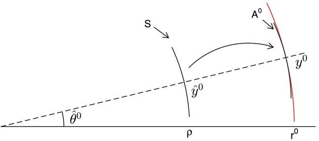
The second order ancillary segment at does not lie on the exact ancillary surface . The tangent vector at the data point is , which is the same as the tangent vector for the exact ancillary and which agrees with the usual tangent vector (see [22]). However, the acceleration vector is , which differs slightly from that for the exact ancillary: the approximation has radius of curvature , as opposed to for the exact, but the difference in moderate deviations about can be seen to be small and is second order.
The second order ancillary contour through can also be expressed in a Taylor series as ; here, the acceleration vector is orthogonal to the velocity vector . Similar results hold in wide generality when has dimension and has dimension ; further examples are discussed in the next section and the general development follows in Sections 4 and 5.
3 Some examples
Example 1 ((Nonlinear regression, known)).
Consider a nonlinear regression model in , where the error is and the regression or solution surface is smooth with parameter of dimension, say, . For given data point , let be the maximum likelihood value. The fitted value is then and the fitted reference value is . The model as presented is already in quantile form; accordingly, are the observed velocity and acceleration arrays, respectively, and the approximate ancillary contour at the data point is which is just a translation of the solution surface For this, we use matrix multiplication to linearly combine the elements in the arrays and .
Example 2 ((Nonlinear regression, circle case)).
As a special case, consider the regression model where the solution surface is a circle of radius about the origin; this is the full-dimension version of the example in Section 2. For notation, let be an orthonormal basis with vectors defining the plane that includes . Then provides rotated coordinates and gives the solution surface in the new coordinates.
There is an exact ancillary given by and ; the corresponding ancillary contour through is a circle of radius through the data point and lying in the plane . The approximate ancillary contour is a segment of a circle of radius through the data point and lying in the same plane. This directly agrees with the simple Normal-on-the-circle example of Section 2.
For the nonlinear regression model, Severini ([29], page 216) proposes an approximate ancillary by using the obvious pivot with the plug-in maximum likelihood value ; we show that this gives a statistic that can be misleading. In the rotated coordinates, the statistic becomes
which has observed value
If we now set the proposed ancillary equal to its observed value, , we obtain and also obtain and . Together, these say that , and thus that the proposed approximate ancillary is exactly equivalent to the original response variable, which is clearly not ancillary. Severini does note “…it does not necessarily follow that is a second-order ancillary statistic since the dimension of increases with .” The consequences of using the plug-in in the pivot are somewhat more serious: the plug-in pivotal approach for this example does not give an approximate ancillary.
Example 3 ((Nonlinear regression, unknown)).
Consider a nonlinear regression model in , where the error is and the solution surface is smooth with surface dimension (see [24]). Let be the observed data point and be the corresponding maximum likelihood value. We then have the fitted regression , the fitted residual , and the fitted reference value which is just the standardized residual.
Example 4 ((The transformation model)).
The transformation model (see, e.g., [14]) provides a paradigm for exact ancillary conditioning. A typical continuous transformation model for a variable has parameter in a smooth transformation group that operates on an -dimensional sample space for ; for illustration, we assume here that the group acts coordinate by coordinate. The natural quantile function for the th coordinate is , where is a coordinate reference variable with a fixed distribution; the linear regression model with known and unknown error scaling are simple examples. With observed data point , let be the maximum likelihood value and the corresponding reference value satisfying . The second order approximate ancillary is then given as , which is just the usual transformation model orbit . If the group does not apply separately to independent coordinates, then the present quantile approach may not be immediately applicable; this raises issues for the construction of the trajectories and also for the construction of default priors (see, e.g., [4]). Some discussion of this in connection with curved parameters will be reported separately. A modification achieved by adding structure to the transformation model is given by the structural model [14]. This takes the reference distribution for as the primary probability space for the model and examines what events on that space are identifiable from an observed response; we do not address here this alternative modelling approach.
Example 5 ((The inverted Cauchy)).
Consider a location-scale model centered at and scaled by with error given by the standard Cauchy; this gives the statistical model
on the real line. For the sampling version, this location-scale model is an example of the transformation model discussed in the preceding Example 4 and the long-accepted ancillary contour is the half-plane (4).
McCullagh [27] uses linear fractional transformation results that show that the inversion takes the Cauchy () model for into a Cauchy () model for , where . He then notes that the usual location-scale ancillary for the derived model does not map back to give the usual location-scale ancillary on the initial space and would thus typically give different inference results for the parameters; he indicates “not that conditioning is a bad idea, but that the usual mathematical formulation is in some respects ad hoc and not completely satisfactory.”
We illustrate this for in Figure 2. For a data point in the upper-left portion of the plane in part (b) for the inverted Cauchy, the observed ancillary contour is shown as a shaded area; it is a half-plane subtended by . When this contour is mapped back to the initial plane in part (a), the contour becomes three disconnected segments with lightly shaded edges indicating the boundaries; in particular, the line with marks 1, 2, 3, 4, 5, 6 becomes three distinct curves again with corresponding marks 1, 2, 3, 4, 5, 6, but two points on the line have no back images. Indeed, the same type of singularity, where a point with a zero coordinate cannot be mapped back, happens for any sample size . Thus the proposed sample space is not one-to-one continuously equivalent to the given sample space: points are left out and points are created. And the quantile function used on the proposed sample space for constructing the ancillary does not exist on the given sample space: indeed, it is not defined at points and is thus not continuous.
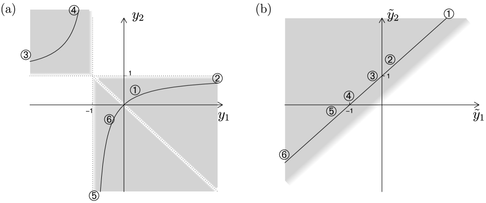
The Cauchy inversion about could equally be about an arbitrary point, say , on the real line and would lead to a corresponding ancillary. We would thus have a wealth of competing ancillaries and a corresponding wealth of inference procedures, and all would have the same lack of one-to-one continuous equivalence to the initial sample space. While Fisher seems not to have explicitly specified continuity as a needed ingredient for typical ancillarity, it also seems unlikely that he would have envisaged ancillarity without continuity. If continuity is included in the prescription for developing the ancillary, then the proposed ancillary for the inverted Cauchy would not arise.
Bayesian statistics involves full conditioning on the observed data and familiar frequentist inference avoids, perhaps even evades, conditioning. Ancillarity, however, represents an intermediate or partial conditioning and, as such, offers a partial bridging of the two extreme approaches to inference.
4 An asymptotic statistic
For the Normal-on-the-circle example, the exact ancillary contour was given as the observed contour of the radial distance : the contour is described implicitly. By contrast, the approximate ancillary was given as the trajectory of a point under change of an index or mathematical parameter : the contour is described explicitly. For the general context, the first approach has serious difficulties, as found even with nonlinear regression, and these difficulties arise with an approximate statistic taking an approximate value; see Example 2. Accordingly, we now turn to the second, the explicit approach, and develop the needed notation and expansions.
Consider a smooth one-dimensional contour through some point . To describe such a contour in the implicit manner requires complementary statistics. By contrast, for the explicit method, we write , which maps a scalar into the sample space . More generally, for a -dimensional contour, we have in , where has dimension and the mapping is again into .
For such a contour, we define the row array of tangent vectors, where the vector gives the direction or gradient of with respect to change in a coordinate . We are interested in such a contour near a particular point ; for convenience, we often choose to be the observed data point and the to be centered so that . In particular, the array of tangent vectors at a particular data point will be of special interest. The vectors in generate a tangent plane at the point and this plane provides a linear approximation to the contour. Differential geometry gives length properties of such vectors as the first fundamental form:
this records the matrix of inner products for the vectors as inherited from the inner product on . A change in the parameterization of the contour will give different tangent vectors , the same tangent plane and a different, but corresponding, first fundamental form.
Now, consider the derivatives of the tangents at :
where is an acceleration or curvature vector relative to coordinates and at . We regard the array as a array of vectors in . We could have used tensor notation, but the approach here has the advantage that we can write the second degree Taylor expansion of at as
| (5) |
which uses matrix multiplication for linearly combining the vectors in the arrays and . Some important characteristics of the quadratic term in (5) are obtained by orthogonalizing the elements of to the tangent plane , to give residuals
this uses the regression analysis projection matrix . The full array of such vectors is then written where is a array of elements ; an element is a vector, which records the regression coefficients of on the vectors .
The array of such orthogonalized curvature vectors is the second fundamental form for the contour at the expansion point. Consider the Taylor expansion (5) and substitute :
where we note that and are being applied to the arrays and by matrix multiplication, but the elements are vectors for and vectors for , and these are being combined linearly. We can then write and thus have the contour expressed in terms of orthogonal curvature vectors with the reparameterization . When we use this in the asymptotic setting, we will have standardized coordinates and the reparameterization will take the form .
5 Verifying second order ancillarity
We have used the Normal-on-the-circle example to illustrate the proposed second order ancillary contour . Now, generally, let be a statistical model with regularity and asymptotic properties as the data dimension increases: we assume that the vector quantile has independent scalar coordinates and is smooth in both the reference variable and the parameter ; more general conditions will be considered subsequently. For the verification, we use a Taylor expansion of the quantile function in terms of both and , and work from theory developed in [5] and [1]. The first steps involve the re-expression of individual coordinates of , , and , and show that the proposed contours establish a partition on the sample space; the subsequent steps establish the ancillarity of the contours. (
-
1a)]
-
(1a)
Standardizing the coordinates. Consider the statistical model in moderate deviations about to order . For this, we work with coordinate departures in units scaled by . Thus, for the th coordinate, we write , and ; and for a modified th quantile coordinate , we Taylor expand to the second order, omit the subscripts and tildes for temporary clarity, and obtain , where is the gradient of with respect to , is the cross Hessian with respect to and , is the Hessian with respect to and vector–matrix multiplication is used for combining with the arrays.
-
(1b)
Re-expressing coordinates for a nicer expansion. We next re-express an coordinate, writing , and then again omit the tildes to obtain the simpler expansion
(6) to order for the modified , and , now in bounded regions about 0.
-
(1c)
Full response vector expansion. For the vector response in quantile form, we can compound the preceding coordinate expansions and write where and are now vectors in , and are arrays of vectors in , is a array of vectors in and is a array of vectors , where the th element of the vector is the product of the th elements of the vectors and .
-
(1d)
Eliminate the cross Hessian: scalar parameter case. The form of a Taylor series depends heavily on how the function and the component variables are expressed. For a particular coordinate of (6) in (1b), if we re-express the coordinate in terms of a modified , substitute it in (6) and then, for notational ease, omit the tildes, we obtain To simplify this, we take the term over to the right-hand side and combine it with to give a re-expressed , take the term over to the right-hand side and choose so that and, finally, combine the terms giving a new . We then obtain with the cross Hessian removed; for this, if , we ignore the coordinate as being ineffective for . For the full response accordingly, we then have to the second order in terms of re-expressed coordinates and . The trajectory of a point is to the second order as varies.
-
(1e)
Scalar case: trajectories form a partition. In the standardized coordinates, the initial data point is with corresponding maximum likelihood value ; the corresponding trajectory is For a general reference value , but with , the trajectory is . The sets with are all translates of and thus form a partition.
Consider an initial point with maximum likelihood value and let be a point in the set . We calculate the trajectory of and show that it lies on ; the partition property then follows and the related Jacobian effect is constant. From the quantile function , we see that the distribution is a -based translation of the reference distribution described by . Thus the likelihood at is , in terms of the log density near . It follows that has maximum likelihood value .
Now, for the trajectory about , we calculate derivatives
which, at the point with , gives
to order . We thus obtain the trajectory of the point :
under variation in . However, with , we have just an arbitrary point on the initial trajectory. Thus the mapping is well defined and the trajectories generate a partition, to second order in moderate derivations in . In the standardized coordinates, the Jacobian effect is constant.
-
(1f)
Vector case: trajectories form a partition. For the vector parameter case, we again use standardized coordinates and choose a parameterization that gives orthogonal curvature vectors at the observed data point . We then examine scalar parameter change on some line through . For this, the results above give a trajectory and any point on it reproduces the trajectory under that scalar parameter. Orthogonality ensures that the vector maximum likelihood value is on the same line just considered. These trajectories are, of course, part of the surface defined by . We then use the partition property of the individual trajectories as these apply perpendicular to the surface; the surfaces are thus part of a partition. We can then write the trajectory of a point as a set
(7) in a partition to the second order in moderate deviations.
-
(2a)
Observed information standardization. With moderate regularity, and following [18] and [23], we have a limiting Normal distribution conditionally on . We then rescale the parameter at to give identity observed information and thus an identity variance matrix for the Normal distribution to second order. We also have a limiting Normal distribution conditionally on ; for this, we linearly modify the vectors in by rescaling and regressing on to give distributional orthogonality to and identity conditional variance matrix to second order.
-
(2b)
The trajectories are ancillary: first derivative parameter change. We saw in the preceding section that key local properties of a statistical model were summarized by the tangent vectors and the curvature vectors , and that the latter can, to advantage, be taken to be orthogonal to the tangent vectors. These vectors give local coordinates for the model and can be replaced by an appropriate subset if linear dependencies are present.
First, consider the conditional model given the directions corresponding to the span . From the ancillary expansion (7), we have that change of to the second order moves points within the linear space ; accordingly, this conditioning is ancillary. Then, consider the further conditioning to an alleged ancillary contour, as described by (7). Also, let be a typical point having as the corresponding maximum likelihood value; is thus on the observed maximum likelihood contour.
Now, consider a rotationally symmetric Normal distribution on the plane with mean on the axis and let be linear in with a quadratic adjustment with respect to . Then is first-derivative ancillary at . For this, we assume, without loss of generality, that the standard deviations are unity. The marginal density for is then
which is symmetric in ; thus showing that the distribution of is first-derivative ancillary at or, more intuitively, that the amount of probability on a contour of is first-derivative free of at . Of course, for this, the -spacing between contours of is constant.
Now, more generally, consider an asymptotic distribution for that is first order rotationally symmetric Normal with mean on the plane; this allows cubic contributions. Also, consider an -dimensional variable which is a quadratic adjustment of . The preceding argument extends to show that is first-derivative ancillary: the two effects are zero and the combination is of the next order.
-
(2c)
Trajectories are ancillary: parameter change in moderate deviations. Now, consider a statistical model with data point and assume regularity, asymptotics and smoothness of the quantile functions. We examine the parameter trajectory in moderate deviations under change in . From the preceding paragraph, we then have first-derivative ancillarity at . But this holds for each expansion in moderate deviations and we thus have ancillarity in moderate deviations. The key here has been to use the expansion form about the point that has equal to the parameter value being examined.
6 Discussion
(
-
iii)]
-
(i)
On ancillarity. The Introduction gave a brief background on ancillary statistics and noted that an ancillary is typically viewed as a statistic with a parameter-free distribution; for some recent discussion, see [17]. Much of the literature is concerned with difficulties that can arise using this third Fisher concept, third after sufficiency and likelihood: that maximizing power given size typically means not conditioning on an ancillary; that shorter on-average confidence intervals typically mean ignoring ancillary conditioning; that techniques that are conditional on an ancillary are often inadmissible; and more. Some of the difficulty may hinge on whether there is merit in the various optimality criteria themselves. However, little in the literature seems focused on the continued evolution and development of this Fisher concept, that is, on what modifications or evolution can continue the exploration initiated in Fisher’s original papers (see [10, 11, 12]).
-
(ii)
On simulations for the conditional model. The second order ancillary in moderate deviations has contours that form a partition, as shown in the preceding section. In the modified or re-expressed coordinates, the contours are in a location relationship and, correspondingly, the Jacobian effect needed for the conditional distribution is constant. However, in the original coordinates, the Jacobian effect would typically not be constant and its effect would be needed for simulations. If the parameter is scalar, then the effect is available to the second order through the divergence function of a vector field; for some discussion and examples, see [15]. For a vector parameter, generalizations can be implemented, but we do not pursue these here.
-
(iii)
Marginal or conditional. When sampling from a scalar distribution having variable and moderate regularity, the familiar central limit theorem gives a limiting Normal distribution for the sample average or sample sum . From a geometric view, we have probability in -space and contours determined by , contours that are planes perpendicular to the -vector. If we then collect the probability on a contour, plus or minus a differential, and deposit it, say, on the intersection of the contour with the span of the -vector, then we obtain a limiting Normal distribution on , using or for location on that line.
A far less familiar Normal limit result applies in the same general context, but with a totally different geometric decomposition. Consider lines parallel to the -vector, the affine cosets of . On these lines, plus or minus a differential, we then obtain a limiting Normal distribution for location say or . In many ways, this conditional, rather than marginal, analysis is much stronger and more useful. The geometry, however, is different, with planes perpendicular to being replaced by points on lines parallel to .
This generalizes giving a limiting conditional Normal distribution on almost arbitrary smooth contours in a partition and it has wide application in recent likelihood inference theory. It also provides third order accuracy rather than the first order accuracy associated with the usual geometry. In a simple sense, planes are replaced by lines or by generalized contours and much stronger, though less familiar, results are obtained. For some background based on Taylor expansions of log-statistical models, see [5, 6] and [1].
Acknowledgements
This research was supported by the Natural Sciences and Engineering Research Council of Canada. The authors wish to express deep appreciation to the referee for very incisive comments. We also offer special thanks to Kexin Ji for many contributions and support with the manuscript and the diagrams.
References
- [1] Andrews, D.F., Fraser, D.A.S. and Wong, A. (2005). Computation of distribution functions from likelihood information near observed data. J. Statist. Plann. Inference 134 180–193. MR2146092
- [2] Barndorff-Nielsen, O.E. (1986). Inference on full or partial parameters based on the standardized log likelihood ratio. Biometrika 73 307–322. MR0855891
- [3] Barndorff-Nielsen, O.E. (1987). Discussion of “Parameter orthogonality and approximate conditional inference.” J. R. Stat. Soc. Ser. B Stat. Methodol. 49 18–20. MR0893334
- [4] Berger, J.O. and Sun, D. (2008). Objective priors for the bivariate normal model. Ann. Statist. 36 963–982. MR2396821
- [5] Cakmak, S., Fraser, D.A.S. and Reid, N. (1994). Multivariate asymptotic model: Exponential and location approximations. Util. Math. 46 21–31. MR1301292
- [6] Cheah, P.K., Fraser, D.A.S. and Reid, N. (1995). Adjustment to likelihood and densities: Calculating significance. J. Statist. Res. 29 1–13. MR1345317
- [7] Cox, D.R. (1980). Local ancillarity. Biometrika 67 279–286. MR0581725
- [8] Cox, D.R. and Reid, N. (1987). Parameter orthogonality and approximate conditional inference. J. R. Stat. Soc. Ser. B Stat. Methodol. 49 1–39. MR0893334
- [9] Daniels, H.E. (1954). Saddle point approximations in statistics. Ann. Math. Statist. 25 631–650. MR0066602
- [10] Fisher, R.A. (1925). Theory of statistical estimation. Proc. Camb. Phil. Soc. 22 700–725.
- [11] Fisher, R.A. (1934). Two new properties of mathematical likelihood. Proc. R. Soc. Lond. Ser. A 144 285–307.
- [12] Fisher, R.A. (1935). The logic of inductive inference. J. R. Stat. Soc. Ser. B Stat. Methodol. 98 39–54.
- [13] Fisher, R.A. (1956). Statistical Methods and Scientific Inference. Edinburgh: Oliver & Boyd.
- [14] Fraser, D.A.S. (1979). Inference and Linear Models. New York: McGraw-Hill. MR0535612
- [15] Fraser, D.A.S. (1993). Directional tests and statistical frames. Statist. Papers 34 213–236. MR1241598
- [16] Fraser, D.A.S. (2003). Likelihood for component parameters. Biometrika 90 327–339. MR1986650
- [17] Fraser, D.A.S. (2004). Ancillaries and conditional inference, with discussion. Statist. Sci. 19 333–369. MR2140544
- [18] Fraser, D.A.S. and Reid, N. (1995). Ancillaries and third order significance. Util. Math. 47 33–53. MR1330888
- [19] Fraser, D.A.S. and Reid, N. (2001). Ancillary information for statistical inference. In Empirical Bayes and Likelihood Inference (S.E. Ahmed and N. Reid, eds.) 185–207. New York: Springer. MR1855565
- [20] Fraser, D.A.S. and Reid, N. (2002). Strong matching for frequentist and Bayesian inference. J. Statist. Plann. Inference 103 263–285. MR1896996
- [21] Fraser, D.A.S., Reid, N., Marras, E. and Yi, G.Y. (2010). Default priors for Bayes and frequentist inference. J. R. Stat. Soc. Ser. B Stat. Methodol. To appear.
- [22] Fraser, D.A.S., Reid, N. and Wu, J. (1999). A simple general formula for tail probabilities for Bayes and frequentist inference. Biometrika 86 249–264. MR1705367
- [23] Fraser, D.A.S. and Rousseau, J. (2008). Studentization and deriving accurate -values. Biometrika 95 1–16. MR2409711
- [24] Fraser, D.A.S., Wong, A. and Wu, J. (1999). Regression analysis, nonlinear or nonnormal: Simple and accurate -values from likelihood analysis. J. Amer. Statist. Assoc. 94 1286–1295. MR1731490
- [25] Lugannani, R. and Rice, S. (1980). Saddlepoint approximation for the distribution of the sum of independent random variables. Adv. in Appl. Probab. 12 475–490. MR0569438
- [26] McCullagh, P. (1984). Local sufficiency. Biometrika 71 233–244. MR0767151
- [27] McCullagh, P. (1992). Conditional inference and Cauchy models. Biometrika 79 247–259. MR1185127
- [28] Reid, N. and Fraser, D.A.S. (2010). Mean likelihood and higher order inference. Biometrika 97. To appear.
- [29] Severini, T.A. (2001). Likelihood Methods in Statistics. Oxford: Oxford Univ. Press. MR1854870