Secrecy Analysis for MISO Broadcast Systems with Regularized Zero-Forcing Precoding

Xin Zhang, Graduate Student Member, IEEE, Shenghui Song, , and Yonina C. Eldar Xin Zhang and Shenghui Song are with the Department of Electronic and Computer Engineering, The Hong Kong University of Science and Technology, Hong Kong (e-mail: xzhangfe@connect.ust.hk; eeshsong@ust.hk).Yonina C. Eldar is with the Faculty of Math and CS, Weizmann Institute of Science, Rehovot 7610001, Israel (e-mail: yonina.eldar@weizmann.ac.il).

Abstract

As an effective way to enhance the physical layer security (PLS) for the broadcast channel (BC), regularized zero-forcing (RZF) precoding has attracted much attention. However, the reliability performance, i.e., secrecy outage probability (SOP), of RZF is not well investigated in the literature. In this paper, we characterize the secrecy performance of RZF precoding in the large multiple-input single-output (MISO) broadcast system. For this purpose, we first consider a central limit theorem (CLT) for the joint distribution of the users’ signal-to-interference-plus-noise ratio (SINR) and the eavesdropper’s (Eve’s) signal-to-noise ratio (ESNR) by leveraging random matrix theory (RMT). The result is then utilized to obtain a closed-form approximation for the ergodic secrecy rate (ESR) and SOP of three typical scenarios: the case with only external Eves, the case with only internal Eves, and that with both. The derived results are then used to evaluate the percentage of users in secrecy outage and the required number of transmit antennas to achieve a positive secrecy rate. It is shown that, with equally-capable Eves, the secrecy loss caused by external Eves is higher than that caused by internal Eves. Numerical simulations validate the accuracy of the theoretical results.

Index Terms:

Physical layer security (PLS), regularized zero-forcing (RZF) precoding, multiple-input single-output (MISO), central limit theorem (CLT), random matrix theory (RMT).

I Introduction

A pivotal problem for wireless communications is eavesdropping due to the broadcast nature of wireless channels [1, 2]. To ensure security, traditional network-layer key-based cryptography has been widely used. However, the dynamics of wireless environments, e.g., fading, lead to issues in key distribution and management, and cause high computational complexity [3]. To provide additional security enhancements, physical layer security (PLS) [4], which utilizes the randomness of the noise and dynamics of the fading channel to limit information leakage to potential eavesdroppers, has been considered as an appealing low-complexity alternative [5].

PLS has become an active area of research, especially in the broadcast channel (BC), where the transmitter tries to broadcast messages to users, with minimum leakage to the eavesdroppers. To this end, linear precoding schemes have been used in confidential transmission of multiple antenna systems due to its simple implementation and effectiveness in interference controlling [6, 7, 8]. In [9, 3], the authors utilized regularized zero-forcing (RZF) precoding, also referred to as regularized channel inversion (RCI), to mitigate the signal leaked to the undesired users and maximize the secrecy sum rate. Despite the wide usage of RZF, its performance analysis is still in the infant stage. Existing works on RZF in MISO BC can be categorized into two types according to the nature of the eavesdroppers, referred to as Eves.

1. Internal Eve: In a MISO BC, users can act maliciously as Eves for other users [10, 11]. Given the Eves are within the BC system, we refer to this scenario as the internal Eve case. Under such circumstances, for a given user, other users are regarded as single-antenna Eves. In [9, 3], the secrecy sum rate of the MISO BC system with internal Eves over independent and identically distributed (i.i.d.) channels was given in closed form by large random matrix theory (RMT). Considering the unequal path loss and correlations of the transmit antennas, the authors of [12] evaluated the secrecy sum rate of RZF using RMT.

2. External Eve: In a practical scenario, external devices can also act as Eves, which are referred to as external Eves. The major difference between internal and external Eves is that the channels of internal Eves are typically correlated with those of the users while the channels of external Eves are typically independent of the users. The impact of external Eves on the secure connectivity was investigated by stochastic geometry (SG) [13, 14, 15]. In [16], assuming that the locations of the Eves are distributed as a Poisson point process (PPP), the authors derived the sum rate and the secrecy outage probability (SOP) with RZF over uncorrelated MISO channels by utilizing RMT and SG. In [17], assuming both users’ and Eves’ locations are distributed as a PPP, the authors derived approximate closed-form results for the SOP and ergodic secrecy rate (ESR) with RZF precoding over uncorrelated MISO channels.

Most existing works focus on the secrecy sum rate of the system [16, 3, 12]. However, the secure reliability performance, i.e., SOP, is not well studied. In [17], the SOP of RZF precoding was derived by SG, considering only large-scale fading, where the impact of small-scale fading on the SOP is ignored. Although the SG based approach is powerful in modeling the dynamics of the network and performing coverage analysis [18], it may not be able to capture long-term behavior of the system where one BS serves a fixed group of users. In this case, the large-scale fading is deterministic and thus the PPP model is not suitable. In particular, the PPP model will dominate the performance analysis such that the impact of small-scale fading can not be fully understood. In this paper, we focus on the impact of small-scale fading on the secrecy performance of MISO BC with RZF precoding and derive the SOP, which is not available in the literature.

A closed-form expression for the SOP is essential for the performance evaluation and will be very beneficial for system design. However, characterization of the secrecy performance, especially the SOP, turns out to be a difficult problem due to the fractional structure of the signal-to-interference-plus-noise ratio (SINR) and the power normalization factor of RZF. In particular, these challenges make it extremely difficult to obtain the closed-form results for the joint distribution of the users’ SINR and Eve’s signal-to-noise ratio (ESNR) in finite dimensions. To overcome this difficulty, asymptotic RMT will be adopted to derive the asymptotic distribution of the SINRs and ESNRs by assuming that the number of transmit antennas, the number of users, and the number of Eves go to infinity with the same pace. In fact, asymptotic RMT has been widely used in large-system analysis of multiple-antenna systems to obtain strikingly simple results [19, 20, 21], which are shown to be effective even for small dimensions.

The contributions of this paper are summarized as follows:

1. We consider a CLT for the joint distribution of the SINRs and ESNRs of a finite number of users and derive explicit expressions for the asymptotic mean and variance. Specifically, we utilize the CLT for the quadratic form and compute the asymptotic second-order attributes by Gaussian tools [20, 22]. The derived results can be extended to the case with imperfect CSI and the analysis of the channel-inversion based precoding method, e.g., secure RZF [23].

2. Based on the CLT, we derive closed-form approximations for the SOP of RZF precoding including three scenarios, namely the External-Eve-Only, Internal-Eve-Only, and External+Internal-Eve cases.

3. The derived results are then used to evaluate how many transmit antennas are needed to guarantee a positive secrecy rate and to estimate the percentage of users in outage. We further compare the performance of RZF for the Internal-Eve-Only and External-Eve-Only cases and derive the theoretical gap between the two secrecy rates, which indicates that the external Eves incur more information leakage than internal ones. Numerical results validate the accuracy of the theoretical results.

The rest of this paper is organized as follows. In Section II, the system model is introduced and the problem is formulated. In Section III, some preliminary results on RMT, which are critical for the derivations in this paper, are given. In Section IV, a CLT for the joint distribution of SINRs and ESNRs and the approximation for the SOP are derived. The derived results are used in Section V to evaluate the percentage of users in outage and the required number of antennas for a positive secrecy rate. Simulation results are provided in Section VI. Section VII concludes the paper.

Notations: Bold, upper case letters and bold, lower case letters represent matrices and vectors, respectively. The probability operator and expectation operator are denoted by $\mathbb{P}(\cdot)$ and $\mathbb{E}(\cdot)$ , respectively. The circularly complex Gaussian distribution and real Gaussian distribution are denoted by $\mathcal{CN}$ and $\mathcal{N}$ , respectively. The $N$ -dimensional complex vector space and real vector space are represented $\mathbb{C}^{N}$ and $\mathbb{R}^{N}$ , respectively. The $M$ -by- $N$ complex and real matrix space, are represented by $\mathbb{C}^{M\times N}$ and $\mathbb{R}^{M\times N}$ , respectively. The centered version of the random variable $x$ is denoted by $\underline{x}=x-\mathbb{E}x$ . $\mathbb{A}^{H}$ denotes the Hermitian transpose of $\mathbb{A}$ and $[{\mathbb{A}}]_{i,j}$ or $A_{ij}$ denotes the $(i,j)$ -th entry. The conjugate of a complex number is represented by $(\cdot)^{*}$ . The spectral norm of $\mathbb{A}$ is given by $\|{\mathbb{A}}\|$ . $\operatorname{Tr}{\mathbb{A}}$ is the trace of ${\mathbb{A}}$ , $\mathbb{I}_{N}$ is the $N$ by $N$ identity matrix, and $\Phi(x)$ represents the cumulative distribution function (CDF) of the standard Gaussian distribution. Almost sure convergence, convergence in probability, and convergence in distribution, are represented by $\xrightarrow[N\rightarrow\infty]{{a.s.}}$ , $\xrightarrow[N\rightarrow\infty]{{i.p.}}$ , and $\xrightarrow[N\rightarrow\infty]{{d}}$ , respectively. The set $\{1,2,...,N\}$ is denoted by $[N]$ and $\mathbbm{1}_{(\cdot)}$ represents the indicator function.

II System Model and Problem Formulation

II-A System Model

We consider the downlink MISO system, where $N$ single-antenna users are served by a base station (BS) with $M$ transmit antennas. We assume that perfect channel state information (CSI) of users is available at the BS and RZF is adopted to suppress information leakage.

RZF is a linear precoding scheme proposed to serve multiple users in the MISO downlink channel, which often demonstrates better performance than ZF, especially with low SNR [6]. With RZF, the received signal at the $k$ -th user is given by

\displaystyle y_{k}=\sqrt{\xi}\mathbb{h}_{k}^{H}\sum_{i=1}^{N}\sqrt{p_{i}}\mathbb{w}_{i}s_{i}+{v}_{k},

(1)

where $s_{i}\sim\mathcal{N}(0,1)$ and $v_{k}\sim\mathcal{N}(0,\sigma^{2})$ denote the transmitted signal for the $i$ -th user and the additive white Gaussian noise (AWGN) at the $k$ -th user, respectively. Here $\mathbb{h}_{k}\in\mathbb{C}^{M}$ and $\mathbb{w}_{i}\in\mathbb{C}^{M}$ represent the channel vector of the $k$ -th user and the precoding vector for the $i$ -th user, respectively, $p_{i}$ denotes the power of the $i$ -th message and $\xi$ represents the power normalization factor. The precoding matrix ${\mathbb{W}}=[\mathbb{w}_{1},\mathbb{w}_{2},...,\mathbb{w}_{N}]\in\mathbb{C}^{M\times N}$ of the RZF precoder is given by [6]

{\mathbb{W}}=\left({\mathbb{H}}{\mathbb{H}}^{H}+z\mathbb{I}_{N}\right)^{-1}{\mathbb{H}},

(2)

where ${\mathbb{H}}=[\mathbb{h}_{1},\mathbb{h}_{2},...,\mathbb{h}_{N}]\in\mathbb{C}^{M\times N}$ and $z>0$ is the regularization parameter of the RZF precoder. The power normalization factor satisfies $\frac{\xi\operatorname{Tr}\mathbb{P}{\mathbb{W}}^{H}{\mathbb{W}}}{N}=1$ , where $\mathbb{P}=\mathrm{diag}(p_{1},p_{2},...,p_{N})$ . The $k$ -th user’s SINR is given by

\text{SINR}_{k}=\frac{p_{k}|\mathbb{h}_{k}^{H}\mathbb{w}_{k}|^{2}}{\sum\limits_{j\neq k}p_{j}|\mathbb{h}_{k}^{H}\mathbb{w}_{j}|^{2}+\frac{\sigma^{2}}{\xi}}.

(3)

Here we consider $L$ single antenna Eves. The channel vector between the BS and the $l$ -th Eve is denoted by $\mathbb{h}_{e,l}\in\mathbb{C}^{M}$ , $l\in[L]$ . The received signal of the $l$ -th Eve, $u_{l}$ , is given by

u_{l}=\sqrt{\xi}\mathbb{h}_{e,l}^{H}\sum_{i=1}^{N}\sqrt{p_{i}}\mathbb{w}_{i}s_{i}+w_{l},

(4)

where $w_{l}\sim\mathcal{N}(0,\rho^{2})$ represents the AWGN at the $l$ -th Eve with $\rho^{2}$ denoting the power of the noise.

It is not straightforward to directly characterize the information leakage, i.e., the information received by the undesired users. Here we consider the worst-case scenario, where all Eves are assumed to work together and be able to cancel out the multiuser interference. This model is widely used in secrecy analysis [3, 12, 24]. Under such circumstances, the ESNR for all Eves to collaboratively overhear the message $s_{k}$ is given by

\text{ESNR}_{k}=\frac{\xi\|{\mathbb{H}}_{e}^{H}\mathbb{w}_{k}\|^{2}}{\rho^{2}},

(5)

where ${\mathbb{H}}_{e}=[\mathbb{h}_{e,1},\mathbb{h}_{e,2},...,\mathbb{h}_{e,L}]$ . The corresponding information leakage rate is given by $C_{e,n}=\log(1+\text{ESNR}_{k})$ . As a result, the secrecy rate of the $k$ -th user is

R_{k}=\lceil\log(1+{\text{SINR}}_{{k}})-\log(1+\text{ESNR}_{k})\rceil^{+}.

(6)

The SOP of the $k$ -th user for a given rate requirement $R$ is given by

P_{out,k}=\mathbb{P}(R_{k}\leq R).

(7)

Note that the Eves can be both internal and external. For the cases with only internal Eves, the channel matrix for the Eves with respect to the $k$ -th user can be given by ${\mathbb{H}}_{e}={\mathbb{H}}_{k}$ , where ${\mathbb{H}}_{k}$ is obtained by removing $\mathbb{h}_{k}$ from ${\mathbb{H}}$ . In this paper, we will evaluate the ESR in (6) and SOP in (7) in a large system setting where the number of transmit antennas and numbers of users and Eves go to infinity with the same space.

II-B Channel Model

We consider a correlated Rayleigh fading channel for users. Accordingly, the channel vector for the $k$ -th user can be represented by $\mathbb{h}_{k}=t_{k}^{\frac{1}{2}}{\mathbb{R}^{\frac{1}{2}}}\mathbb{x}_{k}$ , where $t_{k}$ is the large-scale fading (pathloss) from the BS to the $k$ -th user, $\mathbb{x}_{k}\sim\mathcal{CN}(\mathbb{0},{\mathbb{I}}_{M})$ , and ${\mathbb{R}}$ denotes the correlation matrix of the BS towards the users. In this paper, we assume a common transmit correlation matrix for different users, which is widely used in [12, 25, 26, 27] for tractability of the problem. With the common correlation matrix, the channel matrix ${\mathbb{H}}=[\mathbb{h}_{1},...,\mathbb{h}_{N}]$ is given by

{\mathbb{H}}={\mathbb{R}^{\frac{1}{2}}}{\mathbb{X}}{\mathbb{T}^{\frac{1}{2}}},

(8)

where ${\mathbb{T}}=\mathrm{diag}(t_{1},t_{2},...,t_{N})$ and ${\mathbb{X}}=[\mathbb{x}_{1},...,\mathbb{x}_{N}]$ .

Assume that there are $L$ external single-antenna Eves and denote the channel vector for the $l$ -th Eve as $\mathbb{g}_{l}$ , $l\in[L]$ . Similar to the channel matrix for the users, the channel matrix of the external Eves, ${\mathbb{G}}=[\mathbb{g}_{1},\mathbb{g}_{2},...,\mathbb{g}_{L}]$ , is given by

{\mathbb{G}}={\mathbb{C}}^{\frac{1}{2}}{\mathbb{Y}}{\mathbb{D}}^{\frac{1}{2}},

(9)

where ${\mathbb{C}}\in\mathbb{C}^{M\times M}$ and ${\mathbb{D}}\in\mathbb{C}^{L\times L}=\mathrm{diag}(d_{1},d_{2},...,d_{L})$ represent the correlation matrix and the large-scale fading for the Eves, respectively. Here ${\mathbb{Y}}\in\mathbb{C}^{M\times L}$ is a random matrix with i.i.d. circularly Gaussian entries, i.e., $Y_{m,l}\sim\mathcal{N}(0,\frac{1}{M})$ . Notice that the external Eves overhear the message passively. Thus, we can assume that $\mathbb{h}_{k}$ , $k\in[N]$ and $\mathbb{g}_{l}$ , $l\in[L]$ are independent, i.e., $\mathbb{X}$ and ${\mathbb{Y}}$ are independent. Due to the same reason, the CSI of the Eves is not available at the BS. If there are only external Eves, we have ${\mathbb{H}}_{e}={\mathbb{G}}$ .

In this paper, we consider three typical scenarios.

The External-Eve-Only case. According to (5), we can obtain the ESNR for overhearing message $s_{k}$ as

\text{ESNR}_{ex,k}=\frac{\xi\mathbb{w}_{k}^{H}{\mathbb{G}}{\mathbb{G}}^{H}\mathbb{w}_{k}}{\rho^{2}}.

(10)

The achievable secrecy rate for the $k$ -th user is given by

R_{ex,k}=\lceil\log(1+\text{SINR}_{k})-\log(1+\text{ESNR}_{ex,k})\rceil^{+}.

(11)

The Internal-Eve-Only case. In this case, the unintended users within the MISO BC behave maliciously so that the crosstalk among users causes information leakage [12]. For each user, the other $N-1$ users behave as single-antenna Eves. Specifically, users in $\mathcal{M}_{k}=[N]\setminus{k}$ can cooperate to jointly eavesdrop the message $s_{k}$ . In the worst case scenario, they can be regarded as a single Eve with $N-1$ antennas. The ESNR for overhearing message $s_{k}$ is then given by [9, 3]

\text{ESNR}_{in,k}=\frac{\xi\mathbb{w}_{k}^{H}{\mathbb{H}}_{k}{\mathbb{H}}^{H}_{k}\mathbb{w}_{k}}{\sigma^{2}}.

(12)

The achievable secrecy rate for the $k$ -th user is given by

R_{in,k}=\lceil\log(1+\text{SINR}_{k})-\log(1+\text{ESNR}_{in,k})\rceil^{+}.

(13)

In fact, (11) and (13) can be obtained by taking ${\mathbb{H}}_{e}={\mathbb{G}}$ and ${\mathbb{H}}_{e}={\mathbb{H}}_{k}$ in (6), respectively.

The External+Internal-Eve case. In this case, both the internal and external Eves exist and they work in a non-colluding mode. The secrecy rate of the $k$ -th user is given by [28, 29]

R_{k}=\min(R_{ex,k},R_{in,k}).

(14)

Note that the first two cases are differentiated by whether the channels of the Eves are independent with those of the intended users. The secrecy sum rate of the Intern-Eve-Only case has been investigated in [9, 3, 12] but the SOP is not available in the literature. In the following, we investigate the ESR and SOP for the three cases.

III Preliminaries

In this section, we provide some preliminary results for the evaluation of SINR and ESNR, and introduce the RMT results and notations which will be frequently used in the following derivations. Necessarily, we first introduce the resolvent matrix ${\mathbb{Q}}=(z\mathbb{I}_{N}+{\mathbb{H}}{\mathbb{H}}^{H})^{-1}$ , which will be extensively used in the following analysis. Further define ${\mathbb{Q}}_{k}=(z\mathbb{I}_{N}+{\mathbb{H}}_{k}{\mathbb{H}}_{k}^{H})^{-1}$ , where ${\mathbb{H}}_{k}$ is obtained by removing the $k$ -th column from ${\mathbb{H}}$ . By utilizing the identity $\mathbb{h}_{k}^{H}{\mathbb{Q}}=\frac{\mathbb{h}_{k}^{H}{\mathbb{Q}}_{k}}{1+\mathbb{h}_{k}^{H}{\mathbb{Q}}_{k}\mathbb{h}_{k}}$ , the SINR for $k$ -th user can be rewritten as

\text{SINR}_{k}=\frac{p_{k}A_{k}^{2}}{B_{k}+\sigma^{2}(1+A_{k})^{2}C},

(15)

where $A_{k}=\mathbb{h}_{k}^{H}{\mathbb{Q}}_{k}\mathbb{h}_{k}$ , $B_{k}=\mathbb{h}_{k}^{H}{\mathbb{Q}}_{k}{\mathbb{H}}_{k}{\mathbb{P}}_{k}{\mathbb{H}}_{k}^{H}{\mathbb{Q}}_{k}\mathbb{h}_{k}$ , and $C=\frac{1}{M}\operatorname{Tr}{\mathbb{P}}{\mathbb{H}}^{H}({\mathbb{H}}{\mathbb{H}}^{H}+z\mathbb{I}_{N})^{-2}{\mathbb{H}}$ . Here ${\mathbb{P}}_{k}$ is obtained by removing the $k$ -th row and column of ${\mathbb{P}}=\mathrm{diag}(p_{1},p_{2},...,p_{N})$ . Similarly, $\text{ESNR}_{ex,k}$ and $\text{ESNR}_{in,k}$ can be rewritten as

{\text{ESNR}}_{{ex,k}}=\frac{p_{k}E_{k}}{\rho^{2}C(1+A_{k})^{2}},

(16)

and

{\text{ESNR}}_{{in,k}}=\frac{p_{k}F_{k}}{\sigma^{2}C(1+A_{k})^{2}},

(17)

respectively, where $E_{k}=\mathbb{h}_{k}^{H}{\mathbb{Q}}_{k}{\mathbb{G}}{\mathbb{G}}^{H}{\mathbb{Q}}_{k}\mathbb{h}_{k}$ and $F_{k}=\mathbb{h}_{k}^{H}{\mathbb{Q}}_{k}{\mathbb{H}}_{k}{\mathbb{H}}_{k}^{H}{\mathbb{Q}}_{k}\mathbb{h}_{k}$ . The formulation above resorts the investigation of $\text{SINR}_{k}$ and $\text{ESNR}_{k}$ to that of the $A_{k}$ , $B_{k}$ , $D_{k}$ , and $E_{k}$ , which can be regarded as the quadratic forms of $\mathbb{h}_{k}$ when ${\mathbb{H}}_{k}$ is given. We next introduce three assumptions based on which the analysis in this paper is performed.

Assumption A.1. The dimensions $N$ , $L$ , and $M$ go to infinity at the same pace, i.e., when $M\rightarrow\infty$ ,

		$\displaystyle 0<\lim\inf\frac{M}{N}\leq\frac{M}{N}\leq\lim\sup\frac{M}{N}<\infty,$		(18)
		$\displaystyle 0<\lim\inf\frac{L}{M}\leq\frac{L}{M}\leq\lim\sup\frac{L}{M}<\infty.$		(18)

Assumption A.2. $\|\mathbb{R}\|\leq\infty$ , $\|\mathbb{T}\|\leq\infty$ , $\|{\mathbb{P}}\|\leq\infty$ [30, 31].

Assumption A.3. $\inf\limits_{M\leq 1}\frac{\operatorname{Tr}{\mathbb{R}}}{M}>0$ , $\inf\limits_{M\leq 1}\frac{\operatorname{Tr}{\mathbb{T}}}{M}>0$ , $\inf\limits_{M\leq 1}\frac{\operatorname{Tr}{\mathbb{C}}}{M}>0$ , $\inf\limits_{M\leq 1}\frac{\operatorname{Tr}{\mathbb{D}}}{M}>0$ [20, 32].

Assumption A.1 indicates the asymptotic regime where the number of transmit antennas, the number of users, and the number of external Eves are in the same order. Assumption A.2 and A.3 eliminate the extremely low-rank case of ${\mathbb{R}}$ and ${\mathbb{C}}$ , i.e., the ranks of ${\mathbb{R}}$ and ${\mathbb{C}}$ do not increase with the number of antennas. The bound $\|{\mathbb{P}}\|\leq\infty$ guarantees the power for each message is finite. We further define two ratios $\tau=\frac{M}{N-1}$ and $\theta=\frac{L}{M}$ .

Lemma 1.

Define matrices ${\mathbb{G}}_{R}=\left(z\mathbb{I}_{M}+\widetilde{\delta}{\mathbb{R}}\right)^{-1}$ and ${\mathbb{G}}_{T}=\left(\mathbb{I}_{N}+\widetilde{\delta}{\mathbb{T}}\right)^{-1}$ , where $(\delta,\widetilde{\delta})$ is the unique positive solution for the following system of equations

\begin{cases}\delta&=\frac{1}{M}\operatorname{Tr}{\mathbb{R}}{\mathbb{G}}_{R},\\ \widetilde{\delta}&=\frac{1}{M}\operatorname{Tr}{\mathbb{T}}{\mathbb{G}}_{T}.\end{cases}

(19)

Given assumptions A.1-A.3, for the random matrix ${\mathbb{H}}$ defined in (8), it holds true that for any deterministic matrix $\mathbb{A}$ with bounded norm [30, Theorem 1],

\frac{1}{M}\operatorname{Tr}{\mathbb{A}}{\mathbb{Q}}\xrightarrow[N\rightarrow\infty]{a.s.}\frac{1}{M}\operatorname{Tr}{\mathbb{A}}{\mathbb{G}}_{R},

(20)

and [20, Step B in Section IV]

\frac{1}{M}\mathbb{E}\operatorname{Tr}{\mathbb{A}}{\mathbb{Q}}=\frac{1}{M}\operatorname{Tr}{\mathbb{A}}{\mathbb{G}}_{R}+{\mathcal{O}}(M^{-2}),

(21)

Lemma 1 indicates that the normalized trace of the resolvent converges almost surely to its deterministic equivalent, which is a good approximation for the expectation of the trace of the resolvent. The computation of the variances for the SINR and ESNR is highly related to the trace of the resolvent.

We summarize some frequently used notations in Table I, which are all derived from $\delta$ and $\widetilde{\delta}$ . In the following analysis, some of the symbols have the subscript $k$ . They are derived similarly as those in Table I, but are parameterized by ${\mathbb{R}}$ and ${\mathbb{T}}_{k}$ with

\begin{cases}\delta_{k}&=\frac{1}{M}\operatorname{Tr}{\mathbb{R}}{\mathbb{G}}_{R,k},\\ \widetilde{\delta}_{k}&=\frac{1}{M}\operatorname{Tr}{\mathbb{T}}_{k}{\mathbb{G}}_{T,k},\end{cases}

(22)

where ${\mathbb{T}}_{k}$ is obtained by removing the $k$ -th row and $k$ -th column in ${\mathbb{T}}$ , ${\mathbb{G}}_{R,k}=\left(z\mathbb{I}_{M}+\widetilde{\delta}_{k}{\mathbb{R}}\right)^{-1}$ and ${\mathbb{G}}_{T,k}=\left(\mathbb{I}_{N-1}+{\delta}_{k}{\mathbb{T}}_{k}\right)^{-1}$ . These $k$ -related quantities are used to approximate the ${\mathbb{Q}}_{k}$ related statistics.

TABLE I: List of Notations.

Symbols	Expression	Symbols	Expression
$\gamma$	$\frac{1}{M}\operatorname{Tr}{\mathbb{R}}^{2}{\mathbb{G}}_{R}^{2}$	$\gamma({\mathbb{A}})$	$\frac{1}{M}\operatorname{Tr}{\mathbb{A}}{\mathbb{G}}_{R}^{2}{\mathbb{R}}$
$\widetilde{\gamma}$	$\frac{1}{M}\operatorname{Tr}{\mathbb{T}}^{2}{\mathbb{G}}_{T}^{2}$	$\widetilde{\gamma}({\mathbb{B}})$	$\frac{1}{M}\operatorname{Tr}{\mathbb{B}}{\mathbb{G}}_{T}^{2}{\mathbb{T}}$
$\eta$	$\frac{1}{M}\operatorname{Tr}\mathbb{R}^{3}\mathbb{G}_{R}^{3}$	$\eta({\mathbb{A}})$	$\frac{1}{M}\operatorname{Tr}{\mathbb{A}}{\mathbb{G}}_{R}^{3}{\mathbb{R}}^{2}$
$\widetilde{\eta}$	$\frac{1}{M}\operatorname{Tr}{\mathbb{T}}^{3}\mathbb{G}_{T}^{3}$	$\widetilde{\eta}({\mathbb{B}})$	$\frac{1}{M}\operatorname{Tr}{\mathbb{B}}{\mathbb{G}}_{T}^{3}{\mathbb{T}}^{2}$
$\zeta$	$\frac{1}{M}\operatorname{Tr}\mathbb{R}^{4}\mathbb{G}_{R}^{4}$	$\zeta({\mathbb{A}})$	$\frac{1}{M}\operatorname{Tr}{\mathbb{A}}{\mathbb{G}}_{R}^{4}{\mathbb{R}}^{3}$
$\widetilde{\zeta}$	$\frac{1}{M}\operatorname{Tr}{\mathbb{T}}^{4}\mathbb{G}_{T}^{4}$	$\widetilde{\zeta}({\mathbb{B}})$	$\frac{1}{M}\operatorname{Tr}{\mathbb{B}}{\mathbb{G}}_{T}^{4}{\mathbb{T}}^{3}$

IV Main Results

In this section, we develop theoretical results on the asymptotic distribution of SINR, $\text{ESNR}_{ex}$ , and $\text{ESNR}_{in}$ , and then derive the ESR and SOP of the MISO BC.

IV-A First-order Analysis of the SINR, ESNR, and Secrecy Rate

In this part, we derive approximations for the mean of SINR and ESNR, which will be used to obtain the ESR.

IV-A1 SINR and ESNR

According to (15)-(17), an approximation for SINR, $\text{ESNR}_{ex}$ , and $\text{ESNR}_{in}$ can be obtained by the continuous mapping theorem [33], where we need to obtain the deterministic equivalents of $A_{k}$ , $B_{k}$ , $E_{k}$ , $F_{k}$ , and $C$ .

By Lemma 1 and [34, Lemma 14.2], we have

A_{k}\xrightarrow[N\rightarrow\infty]{a.s.}\frac{t_{k}\mathbb{E}\operatorname{Tr}{\mathbb{R}}{\mathbb{Q}}_{k}}{M}\xrightarrow[]{N\rightarrow\infty}t_{k}\delta_{k}:=\overline{A}_{k},

(23)

and

		$\displaystyle B_{k}\xrightarrow[N\rightarrow\infty]{a.s.}\frac{t_{k}\mathbb{E}\operatorname{Tr}{\mathbb{R}}{\mathbb{Q}}_{k}{\mathbb{H}}_{k}{\mathbb{P}}_{k}{\mathbb{H}}_{k}^{H}{\mathbb{Q}}_{k}}{M}$		(24)
		$\displaystyle=\frac{t_{k}\widetilde{\gamma}_{k}({\mathbb{P}}_{k})\gamma_{k}}{\Delta_{k}}+{\mathcal{O}}(M^{-2}):=\overline{B}_{k}+{\mathcal{O}}(M^{-2}),$		(24)

where $\widetilde{\gamma}_{k}({\mathbb{P}}_{k})$ and $\gamma_{k}$ are given in Table I. Here $\Delta_{k}=1-\gamma_{k}\widetilde{\gamma}_{k}$ ,

C\xrightarrow[N\rightarrow\infty]{a.s.}\frac{\widetilde{\gamma}({\mathbb{P}})\gamma({\mathbb{I}}_{M})}{\Delta}:=\overline{C},

(25)

		$\displaystyle D_{k}\xrightarrow[N\rightarrow\infty]{a.s.}\frac{\mathbb{E}\operatorname{Tr}{\mathbb{R}}{\mathbb{Q}}_{k}{\mathbb{G}}{\mathbb{G}}^{H}{\mathbb{Q}}_{k}}{M}$		(26)
		$\displaystyle=\frac{\theta\overline{d}\gamma_{k}({\mathbb{C}})}{\Delta_{k}}+{\mathcal{O}}(M^{-2}):=\overline{D}_{k}+{\mathcal{O}}(M^{-2}),$		(26)

and

		$\displaystyle E_{k}\xrightarrow[N\rightarrow\infty]{a.s.}\frac{\mathbb{E}\operatorname{Tr}{\mathbb{Q}}_{k}{\mathbb{H}}_{k}{\mathbb{H}}_{k}^{H}{\mathbb{Q}}_{k}{\mathbb{R}}}{M}$		(27)
		$\displaystyle=\frac{\widetilde{\gamma}_{k}({\mathbb{I}}_{N-1})\gamma_{k}}{\Delta_{k}}+{\mathcal{O}}(M^{-2}):=\overline{E}_{k}+{\mathcal{O}}(M^{-2}).$		(27)

We define ${C}_{k}=\frac{\operatorname{Tr}{\mathbb{Q}}_{k}{\mathbb{H}}_{k}{\mathbb{P}}_{k}{\mathbb{H}}^{H}_{k}{\mathbb{Q}}_{k}}{M}$ and its deterministic equivalent is $\overline{{C}}_{k}=\frac{\widetilde{\gamma}_{k}({\mathbb{P}}_{k})\gamma_{k}({\mathbb{I}}_{M})}{\Delta_{k}}$ . In fact, we have

		$\displaystyle\sqrt{M}(C-C_{k})=\sqrt{M}[\frac{p_{k}\mathbb{h}_{k}^{H}{\mathbb{Q}}_{k}^{2}\mathbb{h}_{k}}{M(1+\mathbb{h}_{k}^{H}{\mathbb{Q}}_{k}\mathbb{h}_{k})^{2}}$		(28)
		$\displaystyle+\frac{\mathbb{h}_{k}^{H}{\mathbb{Q}}_{k}{\mathbb{H}}{\mathbb{P}}_{k}{\mathbb{H}}^{H}{\mathbb{Q}}_{k}\mathbb{h}_{k}\mathbb{h}_{k}^{H}{\mathbb{Q}}_{k}\mathbb{h}_{k}}{M(1+\mathbb{h}_{k}^{H}{\mathbb{Q}}_{k}\mathbb{h}_{k})^{2}}$
		$\displaystyle-\frac{2\mathbb{h}_{k}^{H}{\mathbb{Q}}_{k}{\mathbb{H}}{\mathbb{P}}_{k}{\mathbb{H}}^{H}{\mathbb{Q}}_{k}^{2}\mathbb{h}_{k}}{M(1+\mathbb{h}_{k}^{H}{\mathbb{Q}}_{k}\mathbb{h}_{k})}]\xrightarrow[N\rightarrow\infty]{a.s.}{\mathcal{O}}(M^{-\frac{1}{2}}),$

which indicates that $C$ can be replaced by $C_{k}$ in the asymptotic regime A.1. To keep a concise expression for the deterministic equivalent, we will use $\overline{C}_{k}$ instead of $\overline{C}$ .

By the continuous mapping theorem [33], the approximation for $\text{SINR}_{k}$ , $\text{ESNR}_{ex,k}$ , and $\text{ESNR}_{in,k}$ can be obtained by replacing the random quantities with their deterministic equivalents in (23)-(27). Thus, we obtain

$\displaystyle\overline{\text{SINR}}_{k}$	$\displaystyle=\frac{p_{k}t_{k}^{2}\delta_{k}^{2}\Delta_{k}}{\gamma_{k}\widetilde{\gamma}_{k}({\mathbb{P}}_{k})+\sigma^{2}(1+t_{k}\delta_{k})^{2}\gamma_{k}({\mathbb{I}}_{M})\widetilde{\gamma}_{k}({\mathbb{P}}_{k})},$	(29)
$\displaystyle\overline{\text{ESNR}}_{{ex,k}}$	$\displaystyle=\frac{p_{k}\theta\overline{d}\gamma_{k}({\mathbb{C}})}{\rho^{2}(1+t_{k}\delta_{k})^{2}\gamma_{k}({\mathbb{I}}_{M})\widetilde{\gamma}_{k}({\mathbb{P}}_{k})},$
$\displaystyle\overline{\text{ESNR}}_{{in,k}}$	$\displaystyle=\frac{p_{k}\widetilde{\gamma}_{k}({\mathbb{I}}_{N-1})\gamma_{k}}{\sigma^{2}(1+t_{k}\delta_{k})^{2}\widetilde{\gamma}_{k}({\mathbb{P}}_{k})\gamma_{k}({\mathbb{I}}_{M})},$

where $\overline{d}=\frac{\operatorname{Tr}{\mathbb{D}}}{L}$ represents the averaged large-scale fading of the external Eves.

IV-A2 Ergodic Secrecy Rate (ESR)

We approximate the ESR (expectation of the secrecy rate) by replacing the instantaneous SINR and ESNR with their deterministic equivalents in (29) [35]. Specifically, we plug (29) into (11) and (13), respectively, to obtain

$\displaystyle\mathbb{E}R_{in,k}$	$\displaystyle\xrightarrow[]{M\rightarrow\infty}\lceil\overline{C}_{in,k}\rceil^{+},~{}~{}\mathbb{E}R_{ex,k}\xrightarrow[]{M\rightarrow\infty}\lceil\overline{C}_{ex,k}\rceil^{+},$	(30)
$\displaystyle\overline{C}_{in,k}$	$\displaystyle=\log(1+\overline{\text{SINR}}_{k})-\log(1+\overline{\text{ESNR}}_{in,k}),$
$\displaystyle\overline{C}_{ex,k}$	$\displaystyle=\log(1+\overline{\text{SINR}}_{k})-\log(1+\overline{\text{ESNR}}_{ex,k}).$

Note that, the results in this paper are more general than the existing ones, because the spatial correlation at the transmitter and the power allocation scheme are considered. In particular, the above results include the first-order results of previous works [12, Eq. (48)-(50)( $K=1$ )], [9, Eq. (31)], and [3, Theorem 1] as special cases, i.e., by taking ${\mathbb{R}}={\mathbb{I}}_{M}$ , ${\mathbb{T}}={\mathbb{I}}_{N}$ , and ${\mathbb{P}}={\mathbb{I}}_{N}$ .

IV-B Second-order Analysis of the SINR, ESNR, and Secrecy Rate

In this part, we investigate the fluctuations of SINR and ESNR to further investigate the distribution of the secrecy rate. The concerned random quantities, i.e., the SINRs and ESNRs, converge almost surely to a constant as shown in Section IV-A1, which means that their variances vanish when $M$ grows to infinity. In order to investigate the second-order performance, in this section, we show that $\sqrt{M}\text{SINR}_{k}$ and $\sqrt{M}\text{ESNR}_{k}$ converge to a Gaussian distribution when $M$ goes to infinity.

For a finite number $K$ , define SINR, $\text{ESNR}_{ex}$ , and $\text{ESNR}_{in}$ for $K$ users as the vector $\mathbb{g}_{K}\in\mathbb{R}^{3K}$ , given by

		$\displaystyle\mathbb{g}_{K}=(\text{SINR}_{1},\text{SINR}_{2},...,\text{SINR}_{K},\text{ESNR}_{ex,1},\text{ESNR}_{ex,2},$
		$\displaystyle...,\text{ESNR}_{ex,K},\text{ESNR}_{in,1},\text{ESNR}_{in,2},...,\text{ESNR}_{in,K})^{T}.$

In the following, we first derive the joint distribution for the SINRs and ESNRs and then utilize the result to evaluate the SOP.

IV-B1 Joint distribution for SINRs and ESNRs

The following theorem presents the asymptotic joint distribution of $\mathbb{g}_{K}$ .

Theorem 1.

(CLT for the joint distribution of SINRs and ESNRs) For a finite number $K$ , the distribution of the vector $\sqrt{M}\mathbb{g}_{K}$ converges to a Gaussian distribution

\sqrt{M}\left(\mathbb{g}_{K}-\overline{\mathbb{g}}_{K}\right)\xrightarrow[M\rightarrow\infty]{d}\mathcal{N}(\mathbb{0},\mathbb{V}_{K}),

(31)

where

		$\displaystyle\overline{\mathbb{g}}_{K}=(\overline{\text{SINR}}_{1},\overline{\text{SINR}}_{2},...,\overline{\text{SINR}}_{K},\overline{\text{ESNR}}_{ex,1},\overline{\text{ESNR}}_{ex,2},$		(32)
		$\displaystyle...,\overline{\text{ESNR}}_{ex,K},\overline{\text{ESNR}}_{in,1},\overline{\text{ESNR}}_{in,2},...,\overline{\text{ESNR}}_{in,K})^{T}.$		(32)

Here, $\overline{\text{SINR}}_{k}$ , $\overline{\text{ESNR}}_{ex,k}$ , and $\overline{\text{ESNR}}_{in,1}$ are given in (29). The covariance matrix $\mathbb{V}_{K}$ is given by

\mathbb{V}_{K}=\begin{bmatrix}\mathbb{U}_{K}&\mathbb{F}_{K}&\mathbb{J}_{K}\\ \mathbb{F}_{K}&\mathbb{W}_{K}&\mathbb{O}_{K}\\ \mathbb{J}_{K}&\mathbb{O}_{K}&\mathbb{Z}_{K}\end{bmatrix},

(33)

with $\mathbb{U}_{K}=\mathrm{diag}([U_{1},U_{2},...,U_{K}])$ , $\mathbb{W}_{K}=\mathrm{diag}([W_{1},W_{2},...,W_{K}])$ , $\mathbb{Z}_{K}=\mathrm{diag}([Z_{1},Z_{2},...,Z_{K}])$ , $\mathbb{F}_{K}=\mathrm{diag}([F_{1},F_{2},...,F_{K}])$ , $\mathbb{J}_{K}=\mathrm{diag}([J_{1},J_{2},...,J_{K}])$ , and $\mathbb{O}_{K}=\mathrm{diag}([O_{1},O_{2},...,O_{K}])$ . The parameters $U_{k}$ , $W_{k}$ , $V_{k}$ , $F_{k}$ , $J_{k}$ and $O_{k}$ are given by

U_{k}=\frac{a_{k,1}^{2}t_{k}^{2}\gamma_{k}}{\Delta_{k}}+a_{k,2}^{2}t_{k}^{2}\Pi_{k}({\mathbb{P}}_{k})+2a_{k,1}a_{k,2}t_{k}^{2}\kappa_{k}({\mathbb{P}}_{k}),

(34)

	$\displaystyle W_{k}$	$\displaystyle=\frac{a_{k,3}^{2}t_{k}^{2}\gamma_{k}}{\Delta_{k}}+a_{k,4}^{2}t_{k}^{2}[\frac{\theta\overline{d^{2}}\gamma_{k}({\mathbb{C}})^{2}}{\Delta_{k}^{2}}$		(35)
		$\displaystyle+\theta^{2}\overline{d}^{2}\chi_{k}({\mathbb{C}},{\mathbb{C}})]+2a_{k,3}a_{k,4}t_{k}^{2}\theta\overline{d}\Gamma_{k}({\mathbb{C}}),$		(35)

Z_{k}=\frac{a_{k,5}^{2}t_{k}^{2}\gamma_{k}}{\Delta}+a_{k,6}^{2}t_{k}^{2}\Pi_{k}({\mathbb{I}}_{N})+2t_{k}^{2}a_{k,5}a_{k,6}\kappa_{k}({\mathbb{I}}_{N}),

(36)

		$\displaystyle F_{k}=\frac{a_{k,1}a_{k,3}t_{k}^{2}\gamma_{k}}{\Delta_{k}}+a_{k,1}a_{k,4}t_{k}^{2}\theta\overline{d}\Gamma_{k}({\mathbb{C}})$		(37)
		$\displaystyle+a_{k,2}a_{k,3}t_{k}^{2}\kappa_{k}({\mathbb{P}}_{k})+a_{k,2}a_{k,4}t_{k}^{2}\theta\overline{d}\beta_{k}({\mathbb{P}}_{k},{\mathbb{C}}),$		(37)

		$\displaystyle J_{k}=a_{k,1}a_{k,6}t_{k}^{2}\kappa_{k}({\mathbb{I}}_{M})+a_{k,2}a_{k,5}t_{k}^{2}\kappa_{k}({\mathbb{P}}_{k})+$		(38)
		$\displaystyle\frac{a_{k,1}a_{k,5}t_{k}^{2}\gamma_{k}}{\Delta_{k}}+a_{k,2}a_{k,6}t_{k}^{2}[\kappa_{k}({\mathbb{P}}_{k})-z\beta_{k}({\mathbb{P}}_{k},{\mathbb{I}}_{M})],$		(38)

	$\displaystyle O_{k}$	$\displaystyle=\frac{a_{k,3}a_{k,5}t_{k}^{2}\gamma_{k}}{\Delta_{k}}+a_{k,3}a_{k,6}t_{k}^{2}\kappa_{k}({\mathbb{I}}_{N-1})$		(39)
		$\displaystyle+a_{k,4}a_{k,5}t_{k}^{2}\theta\overline{d}\Gamma_{k}({\mathbb{C}})+a_{k,4}a_{k,6}t_{k}^{2}\theta\overline{d}\beta_{k}({\mathbb{I}}_{N-1},{\mathbb{C}}),$		(39)

where $\Pi_{k}(\cdot)$ , $\kappa_{k}(\cdot)$ , $\chi_{k}(\cdot)$ , $\beta_{k}(\cdot)$ , and $\Gamma_{k}(\cdot)$ are given by (90) to (94) in Appendix B. Here, $a_{k,i}$ , $i=1,2,...,6$ are given in (40) at the top of the next page.

	$\displaystyle a_{k,1}$	$\displaystyle\!=\!\frac{2p_{k}[t_{k}\delta\Delta_{k}(t_{k}\gamma_{k}+\sigma^{2}(1+t_{k}\delta_{k})\gamma({\mathbb{I}}_{M}))]}{(t_{k}\gamma_{k}+\sigma^{2}(1+t_{k}\delta_{k})^{2}\gamma_{k}({\mathbb{I}}_{M}))^{2}\widetilde{\gamma}_{k}({\mathbb{P}}_{k})},a_{k,2}\!=\!\frac{-p_{k}t_{k}^{2}\delta^{2}_{k}\Delta^{2}_{k}}{(t_{k}\gamma_{k}+\sigma^{2}(1+t_{k}\delta_{k})^{2}\gamma_{k}({\mathbb{I}}_{M}))\widetilde{\gamma}_{k}({\mathbb{P}}_{k})^{2}},a_{k,3}\!=\!\frac{-2p_{k}t_{k}\overline{d}\gamma_{k}({\mathbb{C}})}{\rho^{2}\widetilde{\gamma}_{k}({\mathbb{P}}_{k})\gamma_{k}({\mathbb{I}}_{M})(1+t_{k}\delta_{k})^{3}},$		(40)
	$\displaystyle a_{k,4}$	$\displaystyle\!=\!\frac{p_{k}\Delta_{k}}{\rho^{2}\widetilde{\gamma}_{k}({\mathbb{P}}_{k})\gamma_{k}({\mathbb{I}}_{M})(1+t_{k}\delta_{k})^{2}},a_{k,5}\!=\!\frac{-2p_{k}t_{k}\widetilde{\gamma}({\mathbb{I}}_{N})\gamma_{k}}{\sigma^{2}\widetilde{\gamma}_{k}({\mathbb{P}}_{k})\gamma_{k}({\mathbb{I}}_{M})(1+t_{k}\delta_{k})^{3}},a_{k,6}\!=\!\frac{p_{k}\Delta_{k}}{\sigma^{2}\widetilde{\gamma}({\mathbb{P}}_{k})\gamma_{k}({\mathbb{I}}_{M})(1+t_{k}\delta_{k})^{2}}.$		(40)

The terms $\chi({\mathbb{C}},{\mathbb{C}})$ , $\Gamma({\mathbb{C}})$ , $\Pi({\mathbb{P}})$ , and $\kappa({\mathbb{P}})$ are the deterministic approximations for $\frac{1}{M}\mathbb{E}\operatorname{Tr}{\mathbb{Q}}{\mathbb{C}}{\mathbb{Q}}{\mathbb{R}}{\mathbb{Q}}{\mathbb{C}}{\mathbb{Q}}{\mathbb{R}}$ , $\frac{1}{M}\mathbb{E}\operatorname{Tr}{\mathbb{Q}}{\mathbb{R}}{\mathbb{Q}}{\mathbb{R}}{\mathbb{Q}}{\mathbb{C}}$ , $\frac{1}{M}\mathbb{E}\operatorname{Tr}({\mathbb{Q}}{\mathbb{R}}{\mathbb{Q}}{\mathbb{H}}{\mathbb{P}}{\mathbb{H}}^{H})^{2}$ , and $\frac{1}{M}\mathbb{E}\operatorname{Tr}{\mathbb{R}}{\mathbb{Q}}{\mathbb{H}}{\mathbb{P}}{\mathbb{H}}^{H}{\mathbb{Q}}{\mathbb{R}}{\mathbb{Q}}$ , respectively, which are proved by Lemma 3 in Appendix B.

Proof.

The proof of Theorem 1 is given in Appendix A. ∎

Theorem 1 indicates that for a finite number of users, i.e., $K\ll M$ , the joint distribution of the SINRs and ESNRs converges to a joint Gaussian distribution when $M$ , $L$ , and $N$ go to infinity with the same pace. From the structure of the covariance matrix $\mathbb{V}_{K}$ , we observe that the SINRs of different users are asymptotically independent. Similar results can also be obtained for the ESNR. However, $\text{SINR}_{k}$ and $\text{ESNR}_{ex,k}$ are not independent, and their covariances are characterized by the diagonal entries of $\mathbb{F}_{K}$ . Similarly, the covariance of the pairs $(\text{SINR}_{k},\text{ESNR}_{in,k})$ and $(\text{ESNR}_{ex,k},\text{ESNR}_{in,k})$ is characterized by the diagonal entries of $\mathbb{J}_{K}$ and $\mathbb{O}_{K}$ , respectively. It follows from Theorem 1 that for a large system, the SINR and ESNR can be approximated by a Gaussian distribution, which will be utilized to evaluate the SOP in the following.

Theorem 1 is obtained by assuming a common correlation matrix as mentioned in Section II-B. When different correlation matrices are assumed, the system of equations in (19) will become a system of $N$ equations parameterized by $N$ different correlation matrices, i.e., ${\mathbb{R}}_{1}$ , ${\mathbb{R}}_{2}$ ,…, ${\mathbb{R}}_{N}$ [35, Eq. (11)] and there will be $N$ different $\delta$ s instead of only one in (19). In this case, the characterization of the higher order trace of resolvents is more complex. For example, $\frac{\mathbb{E}\operatorname{Tr}{\mathbb{Q}}{\mathbb{R}}{\mathbb{Q}}{\mathbb{R}}}{M}\xrightarrow[]{M\rightarrow\infty}\frac{\gamma}{\Delta}$ will become $\frac{\mathbb{E}\operatorname{Tr}{\mathbb{Q}}{\mathbb{R}}_{i}{\mathbb{Q}}{\mathbb{R}}_{j}}{M}\xrightarrow[]{M\rightarrow\infty}[({\mathbb{I}}_{M}-\mathbb{S})^{-1}\mathbb{v}]_{i}$ , where $\mathbb{S}\in\mathbb{R}^{N\times N}$ and $\mathbb{v}\in\mathbb{R}^{N}$ are determined by ${\mathbb{R}}_{1}$ , ${\mathbb{R}}_{2}$ ,…, ${\mathbb{R}}_{N}$ . The inverse matrix $({\mathbb{I}}_{M}-\mathbb{S})^{-1}$ will appear frequently and its order will increase in the computation of high-order resolvents like $\frac{1}{\Delta}$ in (90) to (94). Although the simplified common correlation matrix is considered, Theorem 1 sets up a framework for the second-order analysis of SINRs and ESNRs in the MISO system with RZF, which can also be used to analyze the scenario with imperfect CSI and other channel-inversion based precoding schemes like the secure RZF proposed recently in [23].

IV-B2 SOP Evaluation

Based on Theorem 1, the SOP of the three cases can be obtained by Propositions 1 to 3 as follows, which are not yet available in the literature.

Proposition 1.

(External-Eve-Only) Given a rate threshold $R$ , the SOP of user $k$ with only external Eves can be approximated by

P_{ex,out,k}(R)\approx\phi\left(\frac{\sqrt{M}(R-\overline{C}_{ex,k})}{\sqrt{V_{ex,k}}}\right),

(41)

where $V_{ex,k}=\frac{U_{k}}{(1+\overline{g}_{k})^{2}}+\frac{W_{k}}{(1+\overline{g}_{ex,k})^{2}}-\frac{2F_{k}}{(1+\overline{g}_{k})(1+\overline{g}_{ex,k})}$ .

Proposition 2.

(Internal-Eve-Only) Given a rate threshold $R$ , the SOP of user $k$ with only internal Eves can be approximated by

P_{in,out,k}(R)=\phi\left(\frac{\sqrt{M}(R-\overline{C}_{in,k})}{\sqrt{V_{in,k}}}\right),

(42)

where $V_{in,k}=\frac{U_{k}}{(1+\overline{g}_{k})^{2}}+\frac{Z_{k}}{(1+\overline{g}_{in,k})^{2}}-\frac{2J_{k}}{(1+\overline{g}_{k})(1+\overline{g}_{in,k})}$ .

Proposition 3.

(External+Internal-Eve) Given a rate threshold $R$ , the SOP of user $k$ with both external and internal Eves can be approximated by

		$\displaystyle P_{co,out,k}(R)\approx 1-\int_{R}^{\infty}\int_{R}^{\infty}(2\pi)^{-1}[\det({\mathbb{C}}_{co,k})]^{-\frac{1}{2}}\times$		(43)
		$\displaystyle\exp\left(-\frac{1}{2}(\mathbb{x}-\boldsymbol{\mu}_{co,k})^{T}{\mathbb{C}}^{-1}_{co,k}(\mathbb{x}-\boldsymbol{\mu}_{co,k})\right)\mathrm{d}x_{1}\mathrm{d}x_{2},$		(43)

where $\mathbb{x}=[x_{1},x_{2}]^{T}$ , $\boldsymbol{\mu}_{co,k}=[\overline{C}_{ex,k},\overline{C}_{in,k}]^{T}$ , and ${\mathbb{C}}_{co,k}=\begin{bmatrix}V_{ex,k}&V_{co,k}\\ V_{co,k}&V_{in,k}\end{bmatrix}$ , $V_{co,k}=\frac{U_{k}}{(1+\overline{g}_{k})^{2}}+\frac{O_{k}}{(1+\overline{g}_{ex,k})(1+\overline{g}_{in,k})}-\frac{J_{k}}{(1+\overline{g}_{k})(1+\overline{g}_{in,k})}-\frac{F_{k}}{(1+\overline{g}_{k})(1+\overline{g}_{ex,k})}$ .

Propositions 1-3 follow from Theorem 1 by utilizing the delta-method [36] and indicate that the SOP can be approximated by a Gaussian distribution in the large system setting A.1-A.3.

V Large System Analysis

In this section, we utilize the derived results in Section IV to analyze the impact of the system dimensions. To achieve this goal, we ignore the correlation, pathloss, and power allocation and consider the i.i.d. channel, i.e., ${\mathbb{R}}={\mathbb{I}}_{M}$ , ${\mathbb{T}}={\mathbb{I}}_{N}$ , ${\mathbb{C}}={\mathbb{I}}_{M}$ , ${\mathbb{D}}={\mathbb{I}}_{N}$ , and ${\mathbb{P}}={\mathbb{I}}_{N}$ . In this case, the subscript used to differentiate users can be removed and the system of equations in (22) degenerate to the quadratic equation $z\tau\delta^{2}+(\tau z-\tau+1)\delta-\tau=0$ , whose positive solution is given by

\delta=\frac{\tau-1-\tau z+\sqrt{(\tau-1)^{2}+2(1+\tau)\tau z+z^{2}\tau^{2}}}{2z\tau}.

(44)

In addition, $\delta_{(1)}=\frac{\mathrm{d}\delta}{\mathrm{d}z}$ , $\delta_{(2)}=\frac{\mathrm{d}^{2}\delta}{\mathrm{d}z^{2}}$ , and $\delta_{(3)}=\frac{\mathrm{d}^{3}\delta}{\mathrm{d}z^{3}}$ represent the first to third derivatives of $\delta$ with respect to $z$ . With the setting above, we only need to consider the joint distribution of $\mathbb{g}_{i.i.d}=(\text{SINR},\text{ESNR}_{ex},\text{ESNR}_{in})^{T}$ , and Theorem 1 can be simplified as follows.

Theorem 2.

Given assumption A.1, we have

\sqrt{M}\left(\mathbb{g}_{iid}-\overline{\mathbb{g}}_{iid}\right)\xrightarrow[M\rightarrow\infty]{d}\mathcal{N}(\mathbb{0},\mathbb{V}_{iid}),

(45)

where $\overline{\mathbb{g}}_{iid}=(\overline{g}_{iid},\overline{g}_{iid,ex},\overline{g}_{iid,in})^{T}\in\mathbb{R}^{3}$ is given by

\overline{\mathbb{g}}_{iid}=\left(\frac{\delta[1+z\tau(1+\delta)^{2}]}{1+\sigma^{2}(1+\delta)^{2}},\frac{\tau\theta}{\rho^{2}},\frac{1}{\sigma^{2}(1+\delta)^{2}}\right)^{T}.

(46)

The covariance matrix $\mathbb{V}_{iid}\in\mathrm{C}^{3\times 3}$ is given by

\mathbb{V}_{iid}=\begin{bmatrix}U_{iid}&F_{iid}&J_{iid}\\ F_{iid}&W_{iid}&O_{iid}\\ J_{iid}&O_{iid}&Z_{iid}\end{bmatrix},~{}\text{with}

(47)

	$\displaystyle U_{iid}$	$\displaystyle=-[(a_{1}+a_{2})^{2}\delta_{(1)}+(a_{2}^{2}+a_{1}a_{2})z\delta_{(2)}+\frac{a_{2}^{2}z^{2}\delta_{(3)}}{6}],$
	$\displaystyle W_{iid}$	$\displaystyle=-[a_{3}^{2}\delta_{(1)}-a_{4}^{2}\theta\delta_{(1)}^{2}+\frac{\theta^{2}a_{4}^{2}\delta_{(3)}}{6}-a_{3}a_{4}\theta\delta_{(2)}],$
	$\displaystyle Z_{iid}$	$\displaystyle=-[(a_{5}+a_{6})^{2}\delta_{(1)}+a_{5}a_{6}z\delta_{(2)}+\frac{a_{6}^{2}z^{2}\delta_{(3)}}{6}],$

$\displaystyle F_{iid}$	$\displaystyle=-[(a_{1}+a_{2})a_{3}\delta_{(1)}-\frac{[(a_{1}+a_{2})a_{4}\theta-a_{2}a_{3}z]\delta_{(2)}}{2}$	(48)
	$\displaystyle-\frac{a_{2}a_{4}\theta z\delta_{(3)}}{6}],$
$\displaystyle J_{iid}$	$\displaystyle=-[(a_{1}+a_{2})(a_{5}+a_{6})\delta_{(1)}$
	$\displaystyle+\frac{z(a_{2}a_{5}+a_{1}a_{6}+2a_{2}a_{6})\delta_{(2)}}{2}+\frac{za_{2}a_{6}\delta_{(3)}}{6}],$
$\displaystyle O_{iid}$	$\displaystyle=-[a_{3}(a_{5}+a_{6})\delta_{(1)}+\frac{(za_{3}a_{6}-\theta a_{4}(a_{5}+a_{6}))\delta_{(2)}}{2}$
	$\displaystyle-\frac{za_{4}a_{6}\theta\delta_{(3)}}{6}].$

The parameters $a_{i}$ , $i=1,2,...,6$ , are given as

	$\displaystyle a_{1}$	$\displaystyle=\frac{2\delta[1+\sigma^{2}(1+\delta)]}{[1+\sigma^{2}(1+\delta)^{2}]^{2}(\delta+z\delta_{(1)})},a_{4}=\frac{1}{\rho^{2}(1+\delta)^{2}(\delta+z\delta_{(1)})},$
	$\displaystyle a_{2}$	$\displaystyle=\frac{-\delta^{2}}{[1+\sigma^{2}(1+\delta)^{2}]^{2}(\delta+z\delta_{(1)})^{2}},a_{5}=-\frac{2}{\sigma^{2}(1+\delta)^{3}},$
	$\displaystyle a_{3}$	$\displaystyle=\frac{2\theta\delta_{(1)}}{\rho^{2}(1+\delta)^{3}(\delta+z\delta_{(1)})},a_{6}=\frac{1}{\sigma^{2}(1+\delta)^{2}(\delta+z\delta_{(1)})}.$

The SINR distribution of the MISO BC with RZF was investigated in [37], where the i.i.d channel and equal power allocation are assumed. If we discard $\text{ESNR}_{ex}$ and $\text{ESNR}_{in}$ , the results in Theorem 2 degenerate to [37, Theorem 3]. The outage probability for the i.i.d. case can be obtained by a similar approach as Propositions 1 to 3. In this paper, the joint distribution of SINR and ESNR is investigated with correlated transmit antennas and unequal power allocation.

V-A How many users are in secrecy outage?

Theorem 2 can be utilized to evaluate how many users are in outage. For that purpose, we define the empirical distribution

\alpha_{N,case}(R)=\frac{1}{N}\sum_{i=1}^{N}\mathbbm{1}_{\{R_{case}\leq R\}},

(49)

where $case$ can be either External-Eve-Only or Internal-Eve-Only. Here we consider the External-Eve-Only case and the results for the Internal-Eve-Only case can be obtained similarly. The following proposition is an application of Theorem 2 to compute the quantiles of the users in outage.

Proposition 4.

Given assumptions A.1 to A.3, define $R_{ex}(\sigma^{2},\rho^{2},q)$ and $R_{in}(\sigma^{2},q)$ as

	$\displaystyle R_{ex}(\sigma^{2},\rho^{2},q)$	$\displaystyle=\log(1+\overline{g}_{iid,ex})+\sqrt{\frac{V_{ex,iid}}{M}}\phi^{-1}(q),$		(50)
	$\displaystyle R_{in}(\sigma^{2},q)$	$\displaystyle=\log(1+\overline{g}_{iid,in})+\sqrt{\frac{V_{in,iid}}{M}}\phi^{-1}(q).$		(50)

Then, we have

	$\displaystyle\alpha_{N,ex}(R_{ex}(\sigma^{2},\rho^{2},q))\xrightarrow[M\rightarrow\infty]{a.s.}q,$		(51)
	$\displaystyle\alpha_{N,in}(R_{in}(\sigma^{2},q))\xrightarrow[M\rightarrow\infty]{a.s.}q.$		(51)

Proof.

The result follow from the law of large numbers and Theorem 2. ∎

Proposition 4 indicates that for large $N$ and $M$ , given a target secrecy rate $R_{case}$ and the noise level $\sigma^{2}$ , $\rho^{2}$ , the proportion of the users in outage is approximated by $q$ , where $q$ is obtained by solving equation (50). This means that almost $qN$ users are in outage. Given $\rho^{2}$ and $\sigma^{2}$ , $q$ is an increasing function of $R_{case}$ , which indicates that a larger threshold causes more users in outage.

V-B The Secrecy Loss of the External-Eve-Only and Internal-Eve-Only Cases

Next, we investigate the secrecy loss induced by external and internal Eves. To make a fair comparison, we consider the case where the internal and external Eves are equally powerful, i.e., $L=N-1$ and $\rho^{2}=\sigma^{2}$ , and the precoders have the same $z$ . Under such circumstances, $\overline{g}_{iid,in}\xrightarrow[]{M\rightarrow\infty}\frac{\overline{g}_{iid,ex}}{(1+\delta)^{2}}$ , which indicates that the information leakage due to external Eves is larger than that due to internal Eves. This is because, with only internal Eves, the information received by other users is mitigated by RZF due to its ability to cancel interference. With external Eves, RZF precoder will not be able to cancel the interference since the channels of Eves are independent of those of the users.

It can also be observed from (46) that $\text{ESNR}_{ex}$ is constant when the ratio $\frac{L}{N}$ is a constant. Moreover, $\text{ESNR}_{ex}$ does not depend on the regularization parameter $z$ , indicating that the optimal regularization parameter for maximizing the secrecy sum rate is equivalent to that without considering the Eves, i.e., $R=\sum_{i=1}^{N}\log(1+\text{SINR}_{i})$ . The optimal value of the regularization parameter is $z=\frac{\sigma^{2}}{\tau}$ [38].

V-C How many transmit antennas do we need to achieve a positive secrecy rate?

For the External-Eve-Only case with the optimal regularization parameter $z=\frac{\sigma^{2}}{\tau}$ , the inequality $\mu=\delta>\mu_{ex}$ must hold true, i.e.,

\displaystyle\frac{\tau-1-\sigma^{2}+\sqrt{(\tau-1)^{2}+2(1+\tau)\sigma^{2}+\sigma^{4}}}{2\sigma^{2}}\geq\frac{\tau\theta}{\rho^{2}},

(52)

in order to obtain a positive secrecy rate. From (52), the minimum $\tau$ required for a positive secrecy rate is

\tau^{*}=\frac{\frac{L}{N\rho^{2}}(1+\sigma^{2})+\frac{L^{2}\sigma^{2}}{N^{2}\rho^{4}}}{\frac{L}{N\rho^{2}}+1}.

(53)

This indicates that if $M>N\tau^{*}$ , a positive secrecy rate will be guaranteed. The estimation of $M$ is accurate in the high SNR regime because only the term $4\sigma^{2}$ is omitted in the relaxation. When $\frac{1}{\rho^{2}}\rightarrow\infty$ , $M=N\tau\approx\frac{L\sigma^{2}}{\rho^{2}}$ , we can obtain that $M$ grows with the order ${\mathcal{O}}(\rho^{-2})$ and a larger $L$ requires a higher increasing rate of $M$ .

VI Numerical Results

In this section, the theoretical results derived in Sections IV and V are validated by numerical results. Specifically, the accuracy of the SOP approximation and the evaluation of the percentage of users in secure outage are validated by Monte-Carlo simulations. The impact of the regularization factor $z$ and number of transmit antennas required for a positive secrecy rate are also investigated.

A. Simulation Settings: In the simulation, we consider a uniform linear array of antennas at the BS. According to the model for conventional linear antenna arrays [39], the correlation matrix at the BS can be obtained by

		$\displaystyle[\mathbb{L}(d_{r},\alpha,\nu,N)]_{m,n}$		(54)
		$\displaystyle=\int_{-180}^{180}\frac{1}{\sqrt{2\pi\delta^{2}}}e^{\jmath\frac{2\pi}{\lambda}d_{r}(m-n)\sin(\frac{\pi\phi}{180})-\frac{(\phi-\alpha)^{2}}{2\nu^{2}}}\mathrm{d}\phi,$		(54)

where $m$ and $n$ represent the indices of antennas. Here, $d_{r}$ and $N$ denote the relative antenna spacing (in wavelengths) and the dimension of the matrix, respectively, and $\alpha$ and $\nu^{2}$ represent the mean angle and the mean-square angle spreads, whose units are degree. We adopt the setting $d_{r}=\lambda$ . In the following simulations, the correlation matrices are generated according to (54), i.e., ${\mathbb{R}}=\mathbb{L}(1,\alpha_{R},\nu_{R},M)$ , ${\mathbb{C}}=\mathbb{L}(1,\alpha_{C},\nu_{C},M)$ with $\alpha_{R}=\nu_{R}=10$ and $\alpha_{C}=\nu_{C}=5$ . Without loss of generality, we consider the first user, i.e., $k=1$ .

Following [12], a simple model for the large-scale fading of different users $t_{i}$ , $i=1,2,...,N$ is used, with $t_{i}=a_{i}^{-\eta}$ , where $a_{i}$ represents the distance between the BS and $i$ -th user. The path loss exponent $\eta=3$ is used to model a shadowed urban area [40]. Here we divide the users into $G_{a}$ groups and users in the same group have a common distance. We choose $a_{i}=a^{\lfloor\frac{i-1}{{G_{a}}}\rfloor}$ so that $t_{i}=a^{-\eta\lfloor\frac{i-1}{{G_{a}}}\rfloor}$ . Similarly, $d_{i}$ is generated by $d_{i}=b^{-\eta\lfloor\frac{i-1}{{G_{b}}}\rfloor}$ . The power of each message is given by $p_{i}=c^{\lfloor\frac{i-1}{{G_{c}}}\rfloor}$ and the total power is normalized to be $N$ . In the following, we use the setting $a=1.0772$ , $b=1.1262$ , $c=0.9$ , and $G_{a}=G_{b}=G_{c}=4$ . In the figures, we use the notations “Ana.” and “Sim.” to represent the theoretical and the simulation results, respectively.

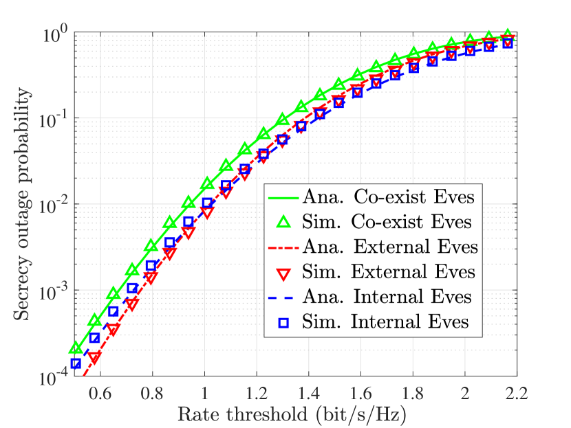
B. The Approximation Accuracy for SOP: In Fig. 1(a), the SOP for three cases are given. The dimensions of the system are set as $M=64$ , $N=32$ , and $L=16$ . The SNRs at the user and external Eves, i.e., $\frac{1}{\sigma^{2}}$ and $\frac{1}{\rho^{2}}$ , are $10$ dB and $4.5$ dB, respectively. The regularization parameter $z$ is set as $z=0.2$ . The number of the Monte-Carlo realizations is $5\times 10^{5}$ . It can be observed that the approximations for the SOP in Proposition 1 to 3 are accurate. The External+Internal-Eve case has the highest SOP and the gap between the External+Internal-Eve case and the other two represents the performance loss induced by different types of Eves.

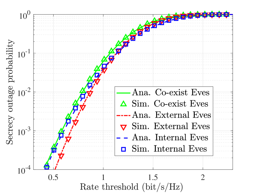
In Fig. 1(b), the SOP of the i.i.d. system is given with the setting $M=64$ , $N=32$ , $L=16$ , $\frac{1}{\sigma^{2}}=6$ dB, and $\frac{1}{\rho^{2}}=2$ dB. This result validates the accuracy of Theorem 2.

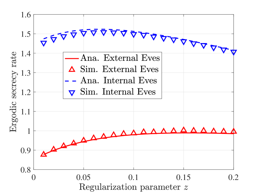
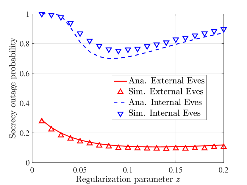
C. Optimal $z$ Control: The theoretical results of this paper can be used to investigate the optimal $z$ for enhancing secure reliability. Figs. 2(a) and 2(b) investigate the impact of $z$ on ESR and SOP for the External-Eve-Only and Internal-Eve-Only case, respectively. Here the i.i.d channel is considered with equal power allocation. The SNR for internal Eves and external Eves are $5$ dB and $2$ dB, respectively. The rate thresholds for the two cases are set as $0.8/\log(2)$ and $1.55/\log(2)$ , respectively. The optimal $z$ that maximizes the ESR can be obtained by $z=\frac{\sigma^{2}}{\tau}$ (External-Eve-Only) and [3, Eq. (12)] (Internal-Eve-Only). The optimal values are determined as $z=0.1532$ and $z=0.0664$ , respectively, which agree with the simulation results shown in Fig. 2(a). It can be observed from Fig. 2 that the optimal $z$ that minimizes the SOP is different from the one that maximizes the ESR.

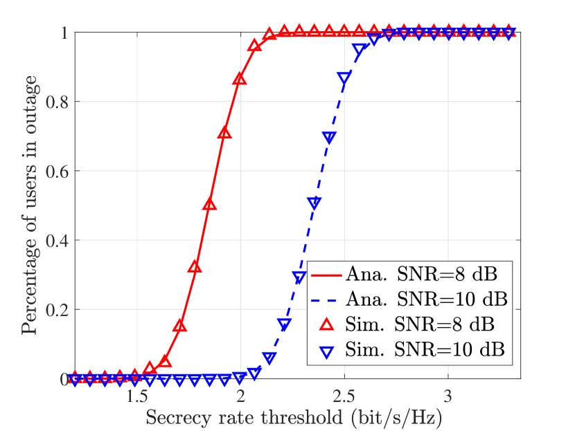
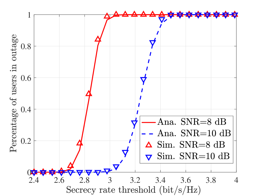
D. Percentage of Users in Outage: Fig. 3(a) and Fig. 3(b) depict percentages of users in outage for the External-Eve-Only and Internal-Eve-Only case, respectively. The parameters are set as $M=256$ , $N=128$ , $L=64$ , $z=0.1$ , and $\frac{1}{\rho^{2}}=4$ dB. It can be observed that the evaluation in (50) matches the empirical result well, which validates the accuracy of Propostion 4 .

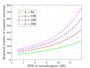
E. The Number of Transmit Antennas Required for a Positive Secrecy: With only the external Eves, Fig. 4 shows the number antennas required to achieve a positive secrecy rate for a given SNR at the Eves. The transmit SNR is set to be $10$ dB and $N=128$ . It can be observed that as the ability of Eves increases, the required number of antennas for a positive secrecy rate increases. The increasing rate grows larger as $L$ increases, which agrees with the analysis in Section V-C.

VII Conclusion

In this paper, the secrecy performance of RZF in the MISO broadcasting system was investigated. In the asymptotic regime that the numbers of transmit antennas, users, and Eves go to infinity with the same pace, a CLT for the joint distribution of SINRs and ESNRs was derived. The CLT was then used to obtain a closed-form approximation for the SOP of three cases, i.e., External-Eve-Only, Internal-Eve-Only, and External+Internal-Eve. Based on the derived results, the required number of transmit antennas for a positive secrecy rate and the percentage of user in secrecy outage were evaluated in a closed form. The secrecy loss caused by the external Eves and internal Eves were compared, showing that the loss caused by the internal Eves is less than that caused by the external Eves. The derived results were validated by numerical simulations. The methods used in this paper can be applied to analyze the performance of RZF with imperfect CSI and investigate the channel-inversion based precoding scheme like the recently proposed secure RZF [23].

Appendix A Proof of Theorem 1

Proof.

The proof can be summarized by three steps including: 1. Show the Gaussianity of the $\text{SINR}_{k}$ ; 2. Show the Gaussianity of the $\text{ESNR}_{k}$ ; and 3. Derive the covariances. In the first two steps, without loss of generosity, we consider user $1$ , i.e., $k=1$ , and the derivation for other users $k=2,...,K$ are the same. The proof of the Gaussianity relies on the CLT for the quadratic forms shown in Lemma 2 of Appendix B. Specifically, we will first show that the SINRs and ESNRs can be approximated by a linear combination of the quadratic forms $A_{k}$ , $B_{k}$ , $E_{k}$ , and $G_{k}$ , and the approximation is tight in probability. The asymptotic variances obtained in this step are related to the high order resolvents, so we need to determine the variance by their deterministic equivalent. This process involves computations for the high-order resolvents, which are summarized by Lemma 3 in Appendix B. The results will also be utilized to evaluate the covariances. Now we turn to the first step.

A-A The Asymptotic Gaussianity of the $\text{SINR}_{1}$

In this step, the fluctuation of $\sqrt{M}(\text{SINR}_{1}-\overline{\text{SINR}}_{1})$ will be investigated. To achieve this goal, we first rewrite $\text{SINR}_{1}-\overline{\text{SINR}}_{1}$ as

		$\displaystyle\text{SINR}_{1}-\overline{\text{SINR}}_{1}=\frac{2p_{1}\overline{A}_{1}(A_{1}-\overline{A}_{1})}{\overline{D}_{1}}$		(55)
		$\displaystyle-\frac{p_{1}\overline{A}_{1}^{2}(D_{1}-\overline{D}_{1})}{\overline{D}^{2}_{1}}+\frac{1}{\sqrt{M}}\varepsilon_{s}.$		(55)

where $\varepsilon_{s}=\sqrt{M}p_{1}D_{1}(\frac{A_{1}}{D_{1}}-\frac{\overline{A}_{1}}{\overline{D}_{1}})^{2}$ . For any given $\epsilon$ , by the Markov inequality, we have

		$\displaystyle\mathbb{P}(\|\varepsilon_{s}\|>\epsilon)\leq\frac{\sqrt{M}}{\epsilon}\mathbb{E}\|D_{1}\|\|\frac{A_{1}}{D_{1}}-\frac{\overline{A}_{1}}{\overline{D}_{1}}\|^{2}$		(56)
		$\displaystyle\leq\frac{2\sqrt{M}}{\epsilon}(\mathbb{E}\frac{\|A_{1}-\overline{A}_{1}\|^{2}}{\|D_{1}\|}+\frac{\|\overline{A}_{1}\|^{2}}{\|\overline{D}_{1}\|^{2}}\mathbb{E}\frac{\|D_{1}-\overline{D}_{1}\|^{2}}{\|D_{1}\|}).$		(56)

Since $|D_{1}|$ is bounded away from zero almost surely, $\mathbb{E}|A_{1}-\overline{A}_{1}|^{2}={\mathcal{O}}(\frac{1}{M^{2}})$ , $\mathbb{E}|A_{1}-\overline{A}_{1}|^{2}={\mathcal{O}}(\frac{1}{M})$ , and $\mathbb{E}|D_{1}-\overline{D}_{1}|^{2}={\mathcal{O}}(\frac{1}{M})$ , we have $\mathbb{P}(|\varepsilon_{s}|>\epsilon)\xrightarrow[]{M\rightarrow\infty}0$ . Therefore, $\sqrt{M}(\text{SINR}_{1}-\overline{\text{SINR}}_{1})$ can be approximated by the first two terms at the right hand side of (LABEL:first_app) and the approximation is tight in probability. $D_{1}$ can be written as

D_{1}-\overline{D}_{1}=B_{1}-\overline{B}_{1}+2\sigma^{2}(1+\overline{A}_{1})\overline{C}(A_{1}-\overline{A}_{1})+\varepsilon_{D},

(57)

where $\varepsilon_{D}=\sigma^{2}(A_{1}-\overline{A}_{1})^{2}C+\sigma^{2}(1+\overline{A}_{1})^{2}(C-\overline{C})$ . By the variance control in [20, 41], we can show that $\mathbb{E}|A_{1}-\overline{A}_{1}|^{4}={\mathcal{O}}(\frac{1}{M^{2}})$ and $\mathbb{E}|C-\overline{C}|^{2}={\mathcal{O}}(\frac{1}{M^{2}})$ so that we can prove $\mathbb{P}(|\varepsilon_{D}|>\epsilon)\xrightarrow[]{M\rightarrow\infty}0$ for a positive $\epsilon$ by the same approach in (LABEL:eps_s). Then, by substituting (57) into (LABEL:first_app), we have the following linear approximation

		$\displaystyle\sqrt{M}(\text{SINR}_{1}-\overline{\text{SINR}}_{1})\xrightarrow[M\rightarrow\infty]{i.p.}$		(58)
		$\displaystyle\sqrt{M}[a_{1,1}(A_{1}-\overline{A}_{1})+a_{1,2}(B_{1}-\overline{B}_{1})],$		(58)

where $a_{1,1}$ and $a_{1,2}$ are given in (40).

Now we turn to determine the asymptotic distribution of the random process at the right hand side of (LABEL:SINR_linear). Given ${\mathbb{H}}_{1}$ , $\sqrt{M}(A_{1}-\overline{A}_{1})$ and $\sqrt{M}(B_{1}-\overline{B}_{1})$ are both in quadratic forms. According to Lemma2, we can show that $\sqrt{M}A_{1}$ and $\sqrt{M}B_{1}$ both converge to a Gaussian distribution when ${\mathbb{H}}_{1}$ is given so that the linear combination of them also converges to a Gaussian distribution. Thus, we only need to determine the asymptotic variances for $\sqrt{M}A_{1}$ , $\sqrt{M}B_{1}$ and their covariance, which can be obtained by Lemma 3 in Appendix B as

V_{A_{1}}=\frac{t_{1}^{2}\operatorname{Tr}{\mathbb{Q}}_{1}{\mathbb{R}}{\mathbb{Q}}_{1}{\mathbb{R}}{\mathbb{Q}}_{1}}{M}\xrightarrow[M\rightarrow\infty]{i.p.}\frac{t_{1}^{2}\gamma_{1}}{\Delta_{1}},

(59)

V_{B_{1}}=\frac{t_{1}^{2}\operatorname{Tr}({\mathbb{Q}}_{1}{\mathbb{R}}{\mathbb{Q}}_{1}{\mathbb{H}}_{1}{\mathbb{P}}_{1}{\mathbb{H}}^{H}_{1})^{2}}{M}\xrightarrow[M\rightarrow\infty]{i.p.}t_{1}^{2}\Pi_{1}({\mathbb{P}}_{1}).

(60)

The covariance of $A_{1}$ and $B_{1}$ can be evaluated by

V_{A_{1},B_{1}}=\frac{t_{1}^{2}\operatorname{Tr}{\mathbb{R}}{\mathbb{Q}}_{1}{\mathbb{R}}{\mathbb{Q}}_{1}{\mathbb{H}}_{1}{\mathbb{P}}_{1}{\mathbb{H}}_{1}^{H}{\mathbb{Q}}_{1}}{M}\xrightarrow[M\rightarrow\infty]{i.p.}t_{1}^{2}\kappa_{1}({\mathbb{P}}_{1}).

(61)

Therefore, we can obtain the asymptotic variance of $\text{SINR}_{1}$ as

U_{1}=a_{1,1}^{2}V_{A_{1}}+a_{1,2}^{2}V_{B_{1}}+2a_{1,1}a_{1,2}V_{A_{1},B_{1}}.

(62)

A-B The Asymptotic Gaussianity of $\text{ESNR}_{ex,1}$

In this part, we will show the Gaussianity of $\text{ESNR}_{ex,1}$ by the same approach as Appendix A-A. We first replace $C$ by $\overline{C}$ in (16) to obtain

\text{ESNR}_{ex,1}=\frac{p_{1}E_{1}}{\rho^{2}\overline{C}(1+A_{1})^{2}}+\varepsilon_{C},

(63)

where $\varepsilon_{C}=\sqrt{M}(\frac{E_{1}}{C(1+A_{1})^{2}}-\frac{E_{1}}{\overline{C}(1+A_{1})^{2}})$ . By the variance control in [22, Lemma 3], we have $\mathrm{Var}(C)={\mathcal{O}}(\frac{1}{M^{2}})$ to show $\varepsilon_{C}\xrightarrow[M\rightarrow\infty]{i.p.}0$ so that we only need to consider the asymptotic distribution of $\frac{\sqrt{M}E_{1}}{(1+A_{1})^{2}}$ . To achieve this goal, we first perform the following decomposition

		$\displaystyle\frac{E_{1}}{(1+A_{1})^{2}}-\frac{\overline{E}_{1}}{(1+\overline{A}_{1})^{2}}=-\frac{2\overline{E}_{1}(A_{1}-\overline{A}_{1})}{(1+\overline{A}_{1})^{3}}$		(64)
		$\displaystyle+\frac{E_{1}-\overline{E}_{1}}{(1+\overline{A}_{1})^{2}}+e_{1}+e_{2}+e_{3},$		(64)

where $e_{1}=\frac{2E_{1}(A_{1}-\overline{A}_{1})^{2}}{(1+A_{1})(1+\overline{A}_{1})^{3}}$ , $e_{2}=\frac{E_{1}(A_{1}-\overline{A}_{1})^{2}}{(1+A_{1})^{2}(1+\overline{A}_{1})^{2}}$ , and $e_{3}=\frac{2(E_{1}-\overline{E}_{1})(\overline{A}_{1}-A_{1})}{(1+\overline{A}_{1})^{3}}$ . We can then show that $e_{1}$ , $e_{2}$ , and $e_{3}$ vanish in probability and here we take $e_{1}$ as an example. $\mathbb{E}\sqrt{M}|e_{1}|$ can be upper bounded by

		$\displaystyle\mathbb{E}\sqrt{M}\|e_{1}\|\leq 2\sqrt{M}(\mathbb{E}\|E_{1}-\overline{E}_{1}\|(A_{1}-\overline{A}_{1})^{2}$		(65)
		$\displaystyle+\overline{E}_{1}\mathbb{E}\|A_{1}-\overline{A}_{1}\|^{2})\leq 2\sqrt{M}(\mathbb{E}^{\frac{1}{2}}(E_{1}-\overline{E}_{1})^{2}\times$
		$\displaystyle\mathbb{E}^{\frac{1}{2}}(A_{1}-\overline{A}_{1})^{4}+\overline{E}_{1}\mathbb{E}\|A_{1}-\overline{A}_{1}\|^{2}).$

The term $(E_{1}-\overline{E}_{1})^{2}$ can be upper bounded by

		$\displaystyle(E_{1}-\overline{E}_{1})^{2}\leq 2[(E_{1}-\frac{t_{1}\operatorname{Tr}{\mathbb{R}}{\mathbb{Q}}_{1}{\mathbb{G}}^{H}{\mathbb{G}}{\mathbb{Q}}_{1}}{M})^{2}$		(66)
		$\displaystyle+(\frac{t_{1}\operatorname{Tr}{\mathbb{R}}{\mathbb{Q}}_{1}{\mathbb{G}}^{H}{\mathbb{G}}{\mathbb{Q}}_{1}}{M}-\overline{E}_{1})^{2}].$		(66)

The first term of the RHS in (66) is bounded by

		$\displaystyle\mathbb{E}\|E_{1}-\frac{t_{1}\operatorname{Tr}{\mathbb{R}}{\mathbb{Q}}_{1}{\mathbb{G}}^{H}{\mathbb{G}}{\mathbb{Q}}_{1}}{M}\|^{2}$		(67)
		$\displaystyle=\frac{t_{1}^{2}\mathbb{E}\operatorname{Tr}({\mathbb{R}}{\mathbb{Q}}_{1}{\mathbb{G}}^{H}{\mathbb{G}}{\mathbb{Q}}_{1})^{2}}{M^{2}}\leq\frac{K\mathbb{E}\\|{\mathbb{G}}\\|^{4}}{M}\overset{(a)}{\leq}\frac{K^{\prime}}{M},$		(67)

where the inequality $(a)$ holds true due to the boundness of $\mathbb{E}\|{\mathbb{G}}\|^{4}$ , which was shown in [22, Lemma 2]. We also have the bound for the second term in the RHS of (66) as

		$\displaystyle\mathbb{E}\|\frac{t_{1}\operatorname{Tr}{\mathbb{R}}{\mathbb{Q}}_{1}{\mathbb{G}}^{H}{\mathbb{G}}{\mathbb{Q}}_{1}}{M}-\overline{E}_{1}\|^{2}\leq 2\mathrm{Var}(\frac{t_{1}\operatorname{Tr}{\mathbb{R}}{\mathbb{Q}}_{1}{\mathbb{G}}^{H}{\mathbb{G}}{\mathbb{Q}}_{1}}{M})$		(68)
		$\displaystyle+2\|\frac{\mathbb{E}t_{1}\operatorname{Tr}{\mathbb{R}}{\mathbb{Q}}_{1}{\mathbb{G}}^{H}{\mathbb{G}}{\mathbb{Q}}_{1}}{M}-\overline{E}_{1}\|^{2}\leq\frac{K^{\prime\prime}}{M^{2}},$		(68)

and

\mathbb{E}|A_{1}-\overline{A}_{1}|^{4}\leq\frac{K^{\prime\prime\prime}}{M^{2}},

(69)

where $K^{\prime}$ , $K^{\prime\prime}$ , and $K^{\prime\prime\prime}$ are constants which are independent of $M$ , $L$ , and $N$ . By substituting (67)-(68) into (66) and then (65), we can obtain that $\sqrt{M}\mathbb{E}|e_{1}|={\mathcal{O}}(M^{-\frac{1}{2}})$ so that

\mathbb{P}(\sqrt{M}|e_{1}|>\varepsilon)\leq\frac{\sqrt{M}\mathbb{E}|e_{1}|}{\varepsilon}\xrightarrow[]{M\rightarrow\infty}0.

(70)

Similarly, we can show that $e_{2}\xrightarrow[M\rightarrow\infty]{i.p.}0$ and $e_{3}\xrightarrow[M\rightarrow\infty]{i.p.}0$ . Therefore, we have

		$\displaystyle\sqrt{M}(\text{ESNR}_{ex,1}-\overline{\text{ESNR}}_{ex,1})\xrightarrow[M\rightarrow\infty]{i.p.}$		(71)
		$\displaystyle\sqrt{M}a_{1,3}(A_{1}-\overline{A}_{1})+\sqrt{M}a_{1,4}(E_{1}-\overline{E}_{1}),$		(71)

V_{E_{1}}=\frac{t_{1}^{2}\operatorname{Tr}({\mathbb{Q}}_{1}{\mathbb{G}}{\mathbb{G}}^{H}{\mathbb{Q}}_{1}{\mathbb{R}})^{2}}{M}\xrightarrow[M\rightarrow\infty]{i.p.}\frac{t_{1}^{2}\mathbb{E}\operatorname{Tr}({\mathbb{Q}}_{1}{\mathbb{G}}{\mathbb{G}}^{H}{\mathbb{Q}}_{1}{\mathbb{R}})^{2}}{M},

(72)

where the last step follows from $\mathrm{Var}(\operatorname{Tr}({\mathbb{Q}}_{1}{\mathbb{G}}{\mathbb{G}}^{H}{\mathbb{Q}}_{1}{\mathbb{R}})^{2})={\mathcal{O}}(1)$ , which can be obtained by the Nash-Poincaré Inequality in [20, 42]. $\frac{\mathbb{E}\operatorname{Tr}({\mathbb{Q}}_{1}{\mathbb{G}}{\mathbb{G}}^{H}{\mathbb{Q}}_{1}{\mathbb{R}})^{2}}{M}$ can be evaluated by the integration by parts formula [20, 42],

		$\displaystyle\frac{\mathbb{E}\operatorname{Tr}{\mathbb{Q}}_{1}{\mathbb{R}}{\mathbb{Q}}_{1}{\mathbb{G}}{\mathbb{G}}^{H}{\mathbb{Q}}_{1}{\mathbb{R}}{\mathbb{Q}}_{1}{\mathbb{G}}{\mathbb{G}}^{H}}{M}$		(73)
		$\displaystyle=\frac{1}{M}\sum_{i,j}\mathbb{E}Y_{i,j}^{*}d_{j}^{\frac{1}{2}}[{\mathbb{C}}^{\frac{1}{2}}{\mathbb{Q}}_{1}{\mathbb{R}}{\mathbb{Q}}_{1}{\mathbb{G}}{\mathbb{G}}^{H}{\mathbb{Q}}{\mathbb{R}}{\mathbb{Q}}_{1}{\mathbb{G}}]_{i,j}$
		$\displaystyle=\frac{(\mathbb{E}\operatorname{Tr}{\mathbb{C}}{\mathbb{Q}}_{1}{\mathbb{R}}{\mathbb{Q}}_{1})^{2}\operatorname{Tr}{\mathbb{D}}^{2}}{M^{3}}$
		$\displaystyle+\frac{(\operatorname{Tr}{\mathbb{D}})^{2}\mathbb{E}\operatorname{Tr}{\mathbb{C}}{\mathbb{Q}}_{1}{\mathbb{R}}{\mathbb{Q}}_{1}{\mathbb{C}}{\mathbb{Q}}_{1}{\mathbb{R}}{\mathbb{Q}}_{1}}{M^{3}}+{\mathcal{O}}(M^{-2}).$

By the evaluations in Lemma 3, we have

V_{E_{1}}\xrightarrow[M\rightarrow\infty]{i.p.}t_{1}^{2}[\frac{\theta\overline{d^{2}}\gamma_{1}({\mathbb{C}})}{\Delta_{1}}+\theta^{2}\overline{d}^{2}\chi_{1}({\mathbb{C}},{\mathbb{C}})],

(74)

V_{A_{1},E_{1}}\!=\!\frac{t_{1}^{2}\operatorname{Tr}{\mathbb{Q}}_{1}{\mathbb{G}}{\mathbb{G}}^{H}{\mathbb{Q}}_{1}{\mathbb{R}}{\mathbb{Q}}_{1}{\mathbb{R}}}{M}\!\xrightarrow[M\rightarrow\infty]{i.p.}\!t_{1}^{2}\theta\overline{d}\Gamma_{1}({\mathbb{C}}).

(75)

Therefore, we can obtain the asymptotic variance of $\text{ESNR}_{ex,1}$ as

W_{1}=a_{1,3}^{2}V_{A_{1}}+a_{1,4}^{2}V_{E_{1}}+2a_{1,3}a_{1,4}V_{A_{1},E_{1}}.

(76)

A-C The Asymptotic Gaussianity of $\text{ESNR}_{in,1}$

Similar to the manipulation of $\text{SINR}_{1}$ and $\text{ESNR}_{ex,1}$ , $\text{ESNR}_{in,1}$ can be approximated by

		$\displaystyle\sqrt{M}(\text{ESNR}_{in,1}-\overline{\text{ESNR}}_{in,1})\xrightarrow[M\rightarrow\infty]{i.p.}$		(77)
		$\displaystyle\frac{\sqrt{M}p_{1}}{\overline{C}}[-\frac{2\overline{F}_{1}(A_{1}-\overline{A}_{1})}{(1+\overline{A}_{1})^{3}}+\frac{F_{1}-\overline{F}_{1}}{(1+\overline{A}_{1})^{2}}]$
		$\displaystyle\xrightarrow[M\rightarrow\infty]{i.p.}\sqrt{M}[a_{1,5}(A_{1}-\overline{A}_{1})+a_{1,6}(F_{1}-\overline{F}_{1})].$

The asymptotic variance of $F_{1}$ and the covariance between $F_{1}$ and $A_{1}$ can be obtained by

	$\displaystyle V_{F_{1}}=\frac{t_{1}^{2}\operatorname{Tr}({\mathbb{Q}}_{1}{\mathbb{H}}_{1}{\mathbb{H}}^{H}_{1}{\mathbb{Q}}_{1}{\mathbb{R}})^{2}}{M}\xrightarrow[M\rightarrow\infty]{i.p.}t_{1}^{2}\Pi_{1}({\mathbb{I}}_{N-1}),$
	$\displaystyle V_{A_{1},F_{1}}=\frac{t_{1}^{2}\operatorname{Tr}{\mathbb{R}}{\mathbb{Q}}_{1}{\mathbb{R}}{\mathbb{Q}}_{1}{\mathbb{H}}_{1}{\mathbb{P}}_{1}{\mathbb{H}}_{1}^{H}{\mathbb{Q}}_{1}}{M}\xrightarrow[M\rightarrow\infty]{i.p.}t_{1}^{2}\kappa_{1}({\mathbb{I}}_{N-1}).$

Therefore, we can obtain the asymptotic variance of $\text{ESNR}_{in,1}$ as

Z_{1}=a_{1,5}^{2}V_{A_{1}}+a_{1,6}^{2}V_{F_{1}}+2a_{1,5}a_{1,6}V_{F_{1},F_{1}}.

A-D The Evaluation of Covariances

We will first give the closed-form expression for the asymptotic covariances between $\text{SINR}_{1}$ , $\text{ESNR}_{in,1}$ , and $\text{ESNR}_{ex,1}$ . By (LABEL:SINR_linear), (LABEL:ex_linear) and (88) in Lemma (3), we can obtain

	$\displaystyle M\mathbb{E}\underline{\text{SINR}_{1}}\underline{\text{ESNR}_{ex,1}}\xrightarrow[]{M\rightarrow\infty}\mathbb{E}(a_{1}a_{3}V_{A_{1}}+$		(78)
	$\displaystyle a_{2}a_{3}V_{A_{1},B_{1}}+a_{1}a_{4}V_{A_{1},E_{1}}+a_{3}a_{3}V_{B_{1},E_{1}}),$		(78)

		$\displaystyle\mathbb{E}V_{B_{1},E_{1}}=\frac{\mathbb{E}\operatorname{Tr}{\mathbb{Q}}_{1}{\mathbb{H}}_{1}{\mathbb{P}}_{1}{\mathbb{H}}^{H}_{1}{\mathbb{Q}}_{1}{\mathbb{R}}{\mathbb{Q}}_{1}{\mathbb{G}}{\mathbb{G}}^{H}{\mathbb{Q}}_{1}{\mathbb{R}}}{M}$		(79)
		$\displaystyle=\frac{\theta\overline{d}\mathbb{E}\operatorname{Tr}{\mathbb{Q}}_{1}{\mathbb{H}}_{1}{\mathbb{P}}_{1}{\mathbb{H}}^{H}_{1}{\mathbb{Q}}_{1}{\mathbb{R}}{\mathbb{Q}}_{1}{\mathbb{C}}{\mathbb{Q}}_{1}{\mathbb{R}}}{M}$
		$\displaystyle=\theta\overline{d}\beta_{1}({\mathbb{P}}_{1},{\mathbb{C}})+{\mathcal{O}}(M^{-2}).$

The evaluations of $V_{A_{1}}$ , $V_{A_{1},B_{1}}$ , and $V_{A_{1},E_{1}}$ can be found in (59), (61), and (75), respectively. The covariances of the pairs $(\text{SINR}_{1},\text{ESNR}_{in,1})$ and $(\text{ESNR}_{ex,1},\text{ESNR}_{in,1})$ can be given by

		$\displaystyle M\mathbb{E}\underline{\text{SINR}_{1}}\underline{\text{ESNR}_{in,1}}\xrightarrow[]{M\rightarrow\infty}\mathbb{E}(a_{1}a_{5}V_{A_{1}}+a_{2}a_{5}V_{A_{1},B_{1}}$
		$\displaystyle+a_{1}a_{4}V_{A_{1},G_{1}}+a_{3}a_{3}V_{B_{1},G_{1}}),$
		$\displaystyle M\mathbb{E}\underline{\text{ESNR}_{ex,1}}\underline{\text{ESNR}_{in,1}}\xrightarrow[]{M\rightarrow\infty}\mathbb{E}(a_{3}a_{5}V_{A_{1}}+$
		$\displaystyle a_{4}a_{5}V_{A_{1},E_{1}}+a_{3}a_{6}V_{A_{1},G_{1}}+a_{4}a_{6}V_{E_{1},G_{1}}),$

where

		$\displaystyle\mathbb{E}V_{B_{1},G_{1}}=\frac{t_{1}^{2}\mathbb{E}\operatorname{Tr}{\mathbb{Q}}_{1}{\mathbb{H}}_{1}{\mathbb{P}}_{1}{\mathbb{H}}_{1}^{H}{\mathbb{Q}}_{1}{\mathbb{R}}{\mathbb{Q}}_{1}{\mathbb{H}}_{1}{\mathbb{H}}_{1}^{H}{\mathbb{Q}}_{1}{\mathbb{R}}}{M}$		(80)
		$\displaystyle\overset{}{=}\frac{t_{1}^{2}\mathbb{E}\operatorname{Tr}{\mathbb{Q}}_{1}{\mathbb{H}}_{1}{\mathbb{P}}_{1}{\mathbb{H}}_{1}^{H}{\mathbb{Q}}_{1}{\mathbb{R}}{\mathbb{Q}}_{1}{\mathbb{R}}}{M}$
		$\displaystyle-\frac{t_{1}^{2}z\mathbb{E}\operatorname{Tr}{\mathbb{Q}}_{1}{\mathbb{H}}_{1}{\mathbb{P}}_{1}{\mathbb{H}}_{1}^{H}{\mathbb{Q}}_{1}{\mathbb{R}}{\mathbb{Q}}_{1}^{2}{\mathbb{R}}}{M}$
		$\displaystyle=t^{2}_{1}[\kappa_{1}({\mathbb{P}}_{1})-z\beta_{1}({\mathbb{I}}_{M},{\mathbb{P}}_{1})]+{\mathcal{O}}(M^{-2}),$

and

		$\displaystyle\mathbb{E}V_{E_{1},G_{1}}=\frac{t_{1}^{2}\mathbb{E}\operatorname{Tr}{\mathbb{Q}}_{1}{\mathbb{H}}_{1}{\mathbb{H}}_{1}^{H}{\mathbb{Q}}_{1}{\mathbb{R}}{\mathbb{Q}}_{1}{\mathbb{G}}{\mathbb{G}}^{H}{\mathbb{Q}}_{1}{\mathbb{R}}}{M}$		(81)
		$\displaystyle=\frac{t_{1}^{2}\theta\overline{d}\mathbb{E}\operatorname{Tr}{\mathbb{Q}}_{1}{\mathbb{H}}_{1}{\mathbb{H}}^{H}_{1}{\mathbb{Q}}_{1}{\mathbb{R}}{\mathbb{Q}}_{1}{\mathbb{C}}{\mathbb{Q}}_{1}{\mathbb{R}}}{M}$
		$\displaystyle=t^{2}_{1}\theta\overline{d}\beta_{1}({\mathbb{I}}_{N-1},{\mathbb{C}})+{\mathcal{O}}(M^{-2}).$

By far, we have shown that $\text{SINR}_{1}$ , $\text{ESNR}_{ex,1}$ , and $\text{ESNR}_{in,1}$ converge to a Gaussian distribution when $M$ , $K$ , $L$ go to infinity with the same pace. Next, we need to investigate the covariance between SINR and ESNR and the covariance between different users. It has been proved in [43, Eq.(2.9)-(2.11)] that $\sqrt{M}A_{i}$ and $\sqrt{M}A_{j}$ are asymptotically independent. By a similar approach, we can also prove the asymptotic independence between $\sqrt{M}B_{i}$ , $\sqrt{M}B_{j}$ , $\sqrt{M}E_{i}$ , $\sqrt{M}E_{j}$ , and $\sqrt{M}G_{i}$ , $\sqrt{M}G_{j}$ when $i\neq j$ so that the asymptotic covariances are all zero. ∎

Appendix B Useful Results

Lemma 2.

(CLT for quadratic forms) Given assumptions A.1, ${\mathbb{H}}_{k}$ , ${\mathbb{G}}$ , and ${\mathbb{P}}$ , there holds true that

\sqrt{M}(A_{k}-\overline{A}_{k})\xrightarrow[M\rightarrow\infty]{d}\mathcal{N}(0,V_{A_{k}}),

(82)

where $V_{A_{k}}=\frac{t_{k}^{2}\operatorname{Tr}{\mathbb{Q}}_{k}{\mathbb{R}}{\mathbb{Q}}_{k}{\mathbb{R}}}{M}$ . Similarly, we also have

	$\displaystyle\sqrt{M}(\overline{B}_{k}-\overline{B}_{k})\xrightarrow[M\rightarrow\infty]{d}\mathcal{N}(0,V_{B_{k}}),$		(83)
	$\displaystyle\sqrt{M}(\overline{E}_{k}-\overline{E}_{k})\xrightarrow[M\rightarrow\infty]{d}\mathcal{N}(0,V_{E_{k}}),$		(83)

where $V_{B_{k}}=\frac{t_{k}^{2}\operatorname{Tr}{\mathbb{R}}{\mathbb{Q}}_{k}{\mathbb{H}}_{k}{\mathbb{P}}_{k}{\mathbb{H}}_{k}^{H}{\mathbb{Q}}_{k}}{M}$ and $V_{E_{k}}=\frac{t_{k}^{2}\operatorname{Tr}{\mathbb{R}}{\mathbb{Q}}_{k}{\mathbb{G}}{\mathbb{G}}^{H}{\mathbb{Q}}_{k}}{M}$ .

Proof.

The first CLT is the separable case in [21] when the resolvent matrix is given. The other two CLTs can be proved by the same approach and the proof is omitted here. ∎

Lemma 3.

(Computation results about the high order resolvents) Given assumptions A.1-A.3 and any deterministic matrices ${\mathbb{C}}$ , ${\mathbb{P}}$ with bounded norm, the following evaluations hold true

\frac{\mathbb{E}\operatorname{Tr}{\mathbb{Q}}{\mathbb{R}}{\mathbb{Q}}{\mathbb{C}}}{M}=\frac{\gamma({\mathbb{C}})}{\Delta}+{\mathcal{O}}(M^{-2}),

(84)

\displaystyle\frac{\mathbb{E}\operatorname{Tr}{\mathbb{Q}}{\mathbb{R}}{\mathbb{Q}}{\mathbb{R}}{\mathbb{Q}}{\mathbb{C}}}{M}=\Gamma({\mathbb{C}})+{\mathcal{O}}(M^{-2}),

(85)

\frac{\mathbb{E}\operatorname{Tr}{\mathbb{R}}{\mathbb{Q}}{\mathbb{H}}{\mathbb{P}}{\mathbb{H}}^{H}{\mathbb{Q}}{\mathbb{R}}{\mathbb{Q}}}{M}=\kappa({\mathbb{P}})+{\mathcal{O}}(M^{-2}),

(86)

\displaystyle\frac{\mathbb{E}\operatorname{Tr}{\mathbb{Q}}{\mathbb{C}}{\mathbb{Q}}{\mathbb{R}}{\mathbb{Q}}{\mathbb{C}}{\mathbb{Q}}{\mathbb{R}}}{M}=\chi({\mathbb{C}},{\mathbb{C}})+{\mathcal{O}}(M^{-2}),

(87)

\displaystyle\frac{\mathbb{E}\operatorname{Tr}{\mathbb{Q}}{\mathbb{H}}{\mathbb{P}}{\mathbb{H}}^{H}{\mathbb{Q}}{\mathbb{R}}{\mathbb{Q}}{\mathbb{C}}{\mathbb{Q}}{\mathbb{R}}}{M}=\beta({\mathbb{P}},{\mathbb{C}})+{\mathcal{O}}(M^{-2}),

(88)

\displaystyle\frac{\mathbb{E}\operatorname{Tr}({\mathbb{Q}}{\mathbb{R}}{\mathbb{Q}}{\mathbb{H}}{\mathbb{P}}{\mathbb{H}}^{H})^{2}}{M}=\Pi({\mathbb{P}})+{\mathcal{O}}(M^{-2}),

(89)

	$\displaystyle\chi({\mathbb{C}},{\mathbb{C}})$	$\displaystyle=\frac{\zeta({\mathbb{C}},{\mathbb{C}})}{\Delta^{2}}+\frac{2\zeta({\mathbb{C}})\gamma({\mathbb{C}})\widetilde{\gamma}}{\Delta^{3}}+\frac{2\eta({\mathbb{C}})^{2}\widetilde{\gamma}}{\Delta^{3}}+\frac{[4\widetilde{\gamma}^{2}\gamma({\mathbb{C}})\eta-3\widetilde{\eta}\gamma\gamma({\mathbb{C}})-\widetilde{\eta}\widetilde{\gamma}\gamma^{2}\gamma({\mathbb{C}})]\eta({\mathbb{C}})}{\Delta^{4}}$		(90)
		$\displaystyle+\frac{\gamma({\mathbb{C}})^{2}(\zeta\widetilde{\gamma}^{2}+\widetilde{\zeta}\gamma^{2}-\eta\widetilde{\eta})}{\Delta^{4}}+\frac{\gamma({\mathbb{C}})^{2}(2\eta^{2}\widetilde{\gamma}^{3}+2\widetilde{\eta}^{2}\gamma^{3}-3\eta\widetilde{\eta}\gamma\widetilde{\gamma}-\eta\widetilde{\eta}\gamma^{2}\widetilde{\gamma}^{2})}{\Delta^{5}}.$		(90)

		$\displaystyle\Pi({\mathbb{P}})=\frac{\gamma^{2}(\widetilde{\eta}({\mathbb{P}}^{2})-\delta\widetilde{\zeta}({\mathbb{P}}^{2}))}{\Delta^{2}}+\frac{2\gamma^{3}\widetilde{\eta}({\mathbb{P}})^{2}+2\gamma^{3}\widetilde{\zeta}({\mathbb{P}})\widetilde{\gamma}({\mathbb{P}})}{\Delta^{3}}+\frac{(\zeta+\gamma^{4}\widetilde{\zeta})\widetilde{\gamma}({\mathbb{P}})^{2}-4(\eta-\gamma^{3}\widetilde{\eta})\gamma\widetilde{\eta}({\mathbb{P}})\widetilde{\gamma}({\mathbb{P}})}{\Delta^{4}}$		(91)
		$\displaystyle+\frac{2\widetilde{\gamma}({\mathbb{P}})^{2}(\widetilde{\gamma}\eta^{2}+\gamma^{5}\widetilde{\eta}^{2}-2\gamma^{2}\eta\widetilde{\eta})}{\Delta^{5}}.$		(91)

		$\displaystyle\beta({\mathbb{P}},{\mathbb{C}})=\frac{2\widetilde{\gamma}({\mathbb{P}})(\widetilde{\gamma}\eta-\gamma^{2}\widetilde{\eta})\eta({\mathbb{C}})+(\widetilde{\gamma}\zeta+\gamma^{3}\widetilde{\zeta})\gamma({\mathbb{C}})\widetilde{\gamma}({\mathbb{P}})-2\widetilde{\eta}({\mathbb{P}})\gamma[\eta({\mathbb{C}})-(\eta({\mathbb{C}})\gamma-\eta\gamma({\mathbb{C}}))\widetilde{\gamma}-\widetilde{\eta}\gamma^{2}\gamma({\mathbb{C}})]}{\Delta^{4}}$		(92)
		$\displaystyle+\frac{\zeta({\mathbb{C}})\widetilde{\gamma}({\mathbb{P}})+\gamma^{2}\gamma({\mathbb{C}})\widetilde{\zeta}({\mathbb{P}})}{\Delta^{3}}+\frac{2[\widetilde{\gamma}^{2}\eta^{2}+\gamma^{4}\widetilde{\eta}^{2}-\gamma(1+\gamma\widetilde{\gamma})\eta\widetilde{\eta}]\gamma({\mathbb{C}})\widetilde{\gamma}({\mathbb{P}})}{\Delta^{5}}.$		(92)

\displaystyle\Gamma({\mathbb{C}})=\frac{\eta({\mathbb{C}})-(\eta({\mathbb{C}})\gamma-\eta\gamma({\mathbb{C}}))\widetilde{\gamma}-\widetilde{\eta}\gamma^{2}\gamma({\mathbb{C}})}{\Delta^{3}},

(93)

\kappa({\mathbb{P}})=\frac{\widetilde{\gamma}({\mathbb{P}})(\eta-\widetilde{\eta}\gamma^{3})}{\Delta^{3}}-\frac{\gamma^{2}\widetilde{\eta}({\mathbb{P}})}{\Delta^{2}}.

(94)

where $\chi({\mathbb{C}},{\mathbb{C}})$ , $\beta({\mathbb{P}},{\mathbb{C}})$ , and $\Pi({\mathbb{P}})$ are given in (90) to (92) at the top of the next page. $\gamma({\mathbb{C}})$ and $\Delta$ are given in Table (I)

Proof.

The proof of Lemma 3 is given in Appendix C. ∎

The evaluation of the high order resolvent is considered in [22], which is used to set up a CLT for the signal-to-noise ratio (SNR) of minimum variance distortionless response (MVDR) filter. (85) is equivalent to [22, Proposition 3]. However, more complex forms for the fourth order resolvents related to multiple system parameters, e.g. ${\mathbb{C}}$ , ${\mathbb{P}}$ , need to be evaluated while in [22], only one undetermined parameter $\mathbb{\Theta}$ is considered. Lemma (3) is more general than those in [22]. If we take the first ${\mathbb{C}}$ to be ${\mathbb{R}}$ , (87) is equivalent to the result in [22, Proposition 4] .

Appendix C Proof of Lemma 3

Proof.

The main idea is to evaluate the high-order resolvents based on the lower-order results. As a result, we will perform the computation from low order to high order iteratively. We first turn to the evaluation of the second-order resolvent in (84). For any deterministic matrices ${\mathbb{A}}$ , ${\mathbb{B}}$ , ${\mathbb{C}}$ , and ${\mathbb{D}}$ with bounded norm, we have

		$\displaystyle\frac{\mathbb{E}\operatorname{Tr}{\mathbb{C}}{\mathbb{Q}}{\mathbb{H}}{\mathbb{A}}{\mathbb{H}}^{H}{\mathbb{D}}{\mathbb{Q}}}{M}=\frac{\operatorname{Tr}{\mathbb{A}}{\mathbb{T}}{\mathbb{G}}_{T}}{M}\frac{\mathbb{E}\operatorname{Tr}{\mathbb{C}}{\mathbb{Q}}{\mathbb{R}}{\mathbb{D}}{\mathbb{Q}}}{M}$		(95)
		$\displaystyle-\frac{\mathbb{E}\operatorname{Tr}{\mathbb{H}}{\mathbb{A}}{\mathbb{T}}{\mathbb{G}}_{T}{\mathbb{H}}^{H}{\mathbb{D}}{\mathbb{Q}}}{M}\frac{\mathbb{E}\operatorname{Tr}{\mathbb{C}}{\mathbb{Q}}{\mathbb{R}}{\mathbb{Q}}}{M}+{\mathcal{O}}(M^{-2})$
		$\displaystyle=\frac{\operatorname{Tr}{\mathbb{A}}{\mathbb{T}}{\mathbb{G}}_{T}}{M}\frac{\operatorname{Tr}{\mathbb{C}}{\mathbb{G}}_{R}{\mathbb{R}}{\mathbb{D}}{\mathbb{G}}_{R}}{M}+\frac{1}{\Delta}(\frac{\operatorname{Tr}{\mathbb{A}}{\mathbb{T}}{\mathbb{G}}_{T}}{M}\widetilde{\gamma}\gamma({\mathbb{C}})$
		$\displaystyle\times\gamma({\mathbb{R}}{\mathbb{D}})-\frac{\operatorname{Tr}{\mathbb{A}}{\mathbb{T}}^{2}{\mathbb{G}}_{T}^{2}\operatorname{Tr}{\mathbb{D}}{\mathbb{R}}{\mathbb{G}}_{R}\gamma({\mathbb{C}})}{M^{2}})+{\mathcal{O}}(M^{-2}),$

by integration by parts formula. Then we turn to evaluate the third-order resolvent. By the resolvent identity and the integration by parts formula, we have

		$\displaystyle z\mathbb{E}[{\mathbb{Q}}{\mathbb{C}}{\mathbb{Q}}{\mathbb{D}}{\mathbb{Q}}]_{i,j}=\mathbb{E}[{\mathbb{Q}}{\mathbb{C}}{\mathbb{Q}}{\mathbb{D}}]_{i,j}-\mathbb{E}[{\mathbb{Q}}{\mathbb{C}}{\mathbb{Q}}{\mathbb{D}}{\mathbb{Q}}{\mathbb{H}}{\mathbb{H}}^{H}]_{i,j}$		(96)
		$\displaystyle=\mathbb{E}\{[{\mathbb{Q}}{\mathbb{C}}{\mathbb{Q}}{\mathbb{D}}]_{i,j}-\widetilde{\delta}[{\mathbb{Q}}{\mathbb{C}}{\mathbb{Q}}{\mathbb{D}}{\mathbb{Q}}{\mathbb{R}}]_{i,j}$
		$\displaystyle+\frac{\operatorname{Tr}{\mathbb{R}}{\mathbb{Q}}{\mathbb{C}}{\mathbb{Q}}{\mathbb{D}}{\mathbb{Q}}}{M}[{\mathbb{Q}}{\mathbb{H}}{\mathbb{T}}{\mathbb{G}}_{T}{\mathbb{H}}^{H}]_{i,j}$
		$\displaystyle+\frac{\operatorname{Tr}{\mathbb{R}}{\mathbb{Q}}{\mathbb{D}}{\mathbb{Q}}}{M}[{\mathbb{Q}}{\mathbb{C}}{\mathbb{Q}}{\mathbb{H}}{\mathbb{T}}{\mathbb{G}}_{T}{\mathbb{H}}^{H}]_{i,j}\}.$

By solving $\mathbb{E}[{\mathbb{Q}}{\mathbb{C}}{\mathbb{Q}}{\mathbb{D}}{\mathbb{Q}}]_{i,j}$ in (96), taking the trace operation, and using variance control in [20, 22], we can obtain

		$\displaystyle\frac{\mathbb{E}\operatorname{Tr}{\mathbb{Q}}{\mathbb{R}}{\mathbb{Q}}{\mathbb{C}}{\mathbb{Q}}{\mathbb{D}}}{M}=\frac{1}{\Delta}(\frac{\mathbb{E}\operatorname{Tr}{\mathbb{Q}}{\mathbb{C}}{\mathbb{Q}}{\mathbb{D}}{\mathbb{R}}{\mathbb{G}}_{R}}{M}$		(97)
		$\displaystyle+\frac{\mathbb{E}\operatorname{Tr}{\mathbb{Q}}{\mathbb{D}}{\mathbb{Q}}{\mathbb{R}}}{M}\frac{\mathbb{E}\operatorname{Tr}{\mathbb{Q}}{\mathbb{C}}{\mathbb{Q}}{\mathbb{H}}{\mathbb{T}}{\mathbb{G}}_{T}{\mathbb{H}}^{H}{\mathbb{R}}{\mathbb{G}}_{R}}{M})+{\mathcal{O}}(M^{-2})$
		$\displaystyle=\frac{1}{\Delta}[\eta({\mathbb{C}},{\mathbb{D}})+\frac{1}{\Delta}(\gamma({\mathbb{C}})\eta({\mathbb{D}})\widetilde{\gamma}+\gamma({\mathbb{D}})\widetilde{\gamma}\eta({\mathbb{C}}))$
		$\displaystyle+\frac{1}{\Delta^{2}}(\gamma({\mathbb{D}})\widetilde{\gamma}^{2}\gamma({\mathbb{C}})\eta-\widetilde{\eta}\gamma\gamma({\mathbb{C}}))]+{\mathcal{O}}(M^{-2}).$

By letting ${\mathbb{D}}={\mathbb{R}}$ in (97), we can obtain (85). Then, by the integration by parts formula [20], we can obtain the evaluation for $\frac{\mathbb{E}\operatorname{Tr}{\mathbb{R}}{\mathbb{Q}}{\mathbb{H}}{\mathbb{A}}{\mathbb{H}}^{H}{\mathbb{D}}{\mathbb{Q}}{\mathbb{C}}{\mathbb{Q}}}{M}$ by plugging (95) into (98) below

		$\displaystyle\frac{\mathbb{E}\operatorname{Tr}{\mathbb{R}}{\mathbb{Q}}{\mathbb{H}}{\mathbb{A}}{\mathbb{H}}^{H}{\mathbb{D}}{\mathbb{Q}}{\mathbb{C}}{\mathbb{Q}}}{M}=\frac{\mathbb{E}\operatorname{Tr}{\mathbb{R}}{\mathbb{Q}}{\mathbb{R}}{\mathbb{D}}{\mathbb{Q}}{\mathbb{C}}{\mathbb{Q}}}{M^{2}}$		(98)
		$\displaystyle\times\operatorname{Tr}{\mathbb{A}}{\mathbb{T}}{\mathbb{G}}_{T}-\frac{\mathbb{E}\operatorname{Tr}{\mathbb{R}}{\mathbb{Q}}{\mathbb{C}}{\mathbb{Q}}\mathbb{E}\operatorname{Tr}{\mathbb{T}}{\mathbb{G}}_{T}{\mathbb{H}}^{H}{\mathbb{D}}{\mathbb{Q}}{\mathbb{R}}{\mathbb{Q}}{\mathbb{H}}{\mathbb{A}}}{M^{2}}$
		$\displaystyle-\frac{\mathbb{E}\operatorname{Tr}{\mathbb{R}}{\mathbb{Q}}{\mathbb{R}}{\mathbb{Q}}{\mathbb{C}}{\mathbb{Q}}\mathbb{E}\operatorname{Tr}{\mathbb{T}}{\mathbb{G}}_{T}{\mathbb{H}}^{H}{\mathbb{D}}{\mathbb{Q}}{\mathbb{H}}{\mathbb{A}}}{M^{2}}+{\mathcal{O}}(M^{-2}).$

By replacing the trace of the third-order resolvents by (97) and letting ${\mathbb{D}}={\mathbb{I}}_{M}$ , ${\mathbb{A}}={\mathbb{P}}$ , ${\mathbb{C}}={\mathbb{R}}$ in (98), we can obtain (86). The fourth-order resolvent in (87) can be evaluated by the similar approach, which is given in (99) at the top of the next page,

		$\displaystyle\frac{\mathbb{E}\operatorname{Tr}{\mathbb{Q}}{\mathbb{C}}{\mathbb{Q}}{\mathbb{R}}{\mathbb{Q}}{\mathbb{C}}{\mathbb{Q}}{\mathbb{R}}}{M}\!=\!\frac{1}{\Delta}\![\frac{\mathbb{E}\operatorname{Tr}{\mathbb{R}}{\mathbb{Q}}{\mathbb{R}}{\mathbb{Q}}{\mathbb{C}}{\mathbb{Q}}}{M}\frac{\mathbb{E}\operatorname{Tr}{\mathbb{Q}}{\mathbb{C}}{\mathbb{Q}}{\mathbb{H}}{\mathbb{T}}{\mathbb{G}}_{T}{\mathbb{H}}^{H}{\mathbb{G}}_{R}{\mathbb{R}}}{M}\!+\!\frac{\mathbb{E}\operatorname{Tr}{\mathbb{R}}{\mathbb{Q}}{\mathbb{C}}{\mathbb{Q}}}{M}\frac{\mathbb{E}\operatorname{Tr}{\mathbb{Q}}{\mathbb{C}}{\mathbb{Q}}{\mathbb{R}}{\mathbb{Q}}{\mathbb{H}}{\mathbb{T}}{\mathbb{G}}_{T}{\mathbb{H}}^{H}{\mathbb{G}}_{R}{\mathbb{R}}}{M}]\!+\!{\mathcal{O}}({M^{-2}})$		(99)
		$\displaystyle\overset{(a)}{=}\frac{1}{\Delta^{4}}\{\gamma({{\mathbb{C}}})[\zeta({\mathbb{C}})\Delta+\zeta\widetilde{\gamma}\gamma({\mathbb{C}})+\zeta(\eta({\mathbb{C}})\widetilde{\gamma}\Delta+\widetilde{\gamma}^{2}\eta\gamma({\mathbb{C}})-\gamma({\mathbb{C}})\gamma\widetilde{\eta})+[\eta({\mathbb{C}})-(\eta({\mathbb{C}})\gamma-\eta\gamma({\mathbb{C}}))\widetilde{\gamma}-\widetilde{\eta}\gamma^{2}\gamma({\mathbb{C}})]]\}+{\mathcal{O}}(M^{-2}),$		(99)

where step $(a)$ in (99) is obtained by plugging (97) and (98) into (99) to replace $\frac{\mathbb{E}\operatorname{Tr}{\mathbb{R}}{\mathbb{Q}}{\mathbb{R}}{\mathbb{Q}}{\mathbb{C}}{\mathbb{Q}}}{M}$ and $\frac{\mathbb{E}\operatorname{Tr}{\mathbb{Q}}{\mathbb{C}}{\mathbb{Q}}{\mathbb{R}}{\mathbb{Q}}{\mathbb{H}}{\mathbb{T}}{\mathbb{G}}_{T}{\mathbb{H}}^{H}{\mathbb{G}}_{R}{\mathbb{R}}}{M}$ , respectively. To obtain (88), we first follow similar steps as in (96) to obtain the evaluation for $\frac{\mathbb{E}\operatorname{Tr}{\mathbb{Q}}{\mathbb{R}}{\mathbb{Q}}{\mathbb{C}}{\mathbb{Q}}{\mathbb{R}}{\mathbb{Q}}{\mathbb{R}}}{M}$ . Then by replacing the third-order terms in

		$\displaystyle\frac{\mathbb{E}\operatorname{Tr}{\mathbb{Q}}{\mathbb{R}}{\mathbb{Q}}{\mathbb{C}}{\mathbb{Q}}{\mathbb{R}}{\mathbb{Q}}{\mathbb{H}}{\mathbb{A}}{\mathbb{H}}^{H}}{M}$		(100)
		$\displaystyle=-\frac{\mathbb{E}\operatorname{Tr}{\mathbb{Q}}{\mathbb{R}}{\mathbb{Q}}{\mathbb{R}}}{M}\frac{\mathbb{E}\operatorname{Tr}{\mathbb{T}}{\mathbb{G}}_{T}{\mathbb{H}}^{H}{\mathbb{Q}}{\mathbb{C}}{\mathbb{Q}}{\mathbb{R}}{\mathbb{Q}}{\mathbb{H}}{\mathbb{A}}}{M}$
		$\displaystyle-\frac{\mathbb{E}\operatorname{Tr}{\mathbb{Q}}{\mathbb{R}}{\mathbb{Q}}{\mathbb{C}}{\mathbb{Q}}{\mathbb{R}}}{M}\frac{\mathbb{E}\operatorname{Tr}{\mathbb{T}}{\mathbb{G}}_{T}{\mathbb{H}}^{H}{\mathbb{Q}}{\mathbb{R}}{\mathbb{Q}}{\mathbb{H}}{\mathbb{A}}}{M}$
		$\displaystyle+\frac{\mathbb{E}\operatorname{Tr}{\mathbb{Q}}{\mathbb{R}}{\mathbb{Q}}{\mathbb{C}}{\mathbb{Q}}{\mathbb{R}}{\mathbb{Q}}{\mathbb{R}}}{M}\frac{\operatorname{Tr}{\mathbb{A}}{\mathbb{T}}{\mathbb{G}}_{T}^{2}}{M}+{\mathcal{O}}(M^{-2}),$

by (97) and (98), we can conclude (88). The tedious computation is omitted here. Then we turn to evaluate (89). By the integration by parts formula, we can obtain

		$\displaystyle\frac{\mathbb{E}\operatorname{Tr}{\mathbb{Q}}{\mathbb{R}}{\mathbb{Q}}{\mathbb{H}}{\mathbb{A}}{\mathbb{H}}^{H}{\mathbb{Q}}{\mathbb{R}}{\mathbb{Q}}{\mathbb{H}}{\mathbb{B}}{\mathbb{H}}^{H}}{M}=$		(101)
		$\displaystyle-\frac{\mathbb{E}\operatorname{Tr}{\mathbb{Q}}{\mathbb{R}}{\mathbb{Q}}{\mathbb{R}}}{M}\frac{\mathbb{E}\operatorname{Tr}{\mathbb{T}}{\mathbb{G}}_{T}{\mathbb{H}}^{H}{\mathbb{Q}}{\mathbb{H}}{\mathbb{A}}{\mathbb{H}}^{H}{\mathbb{Q}}{\mathbb{R}}{\mathbb{Q}}{\mathbb{H}}{\mathbb{B}}}{M}$
		$\displaystyle+\frac{\mathbb{E}\operatorname{Tr}{\mathbb{Q}}{\mathbb{R}}{\mathbb{Q}}{\mathbb{R}}\mathbb{E}\operatorname{Tr}{\mathbb{T}}{\mathbb{G}}_{T}{\mathbb{A}}{\mathbb{H}}^{H}{\mathbb{Q}}{\mathbb{R}}{\mathbb{Q}}{\mathbb{H}}{\mathbb{B}}}{M^{2}}$
		$\displaystyle-\frac{\mathbb{E}\operatorname{Tr}{\mathbb{R}}{\mathbb{Q}}{\mathbb{R}}{\mathbb{Q}}{\mathbb{H}}{\mathbb{A}}{\mathbb{H}}^{H}{\mathbb{Q}}}{M}\frac{\mathbb{E}\operatorname{Tr}{\mathbb{T}}{\mathbb{G}}_{T}{\mathbb{H}}^{H}{\mathbb{Q}}{\mathbb{R}}{\mathbb{Q}}{\mathbb{H}}{\mathbb{B}}}{M}$
		$\displaystyle-\frac{\mathbb{E}\operatorname{Tr}{\mathbb{R}}{\mathbb{Q}}{\mathbb{R}}{\mathbb{Q}}{\mathbb{H}}{\mathbb{A}}{\mathbb{H}}^{H}{\mathbb{Q}}{\mathbb{R}}{\mathbb{Q}}}{M}\frac{\mathbb{E}\operatorname{Tr}{\mathbb{T}}{\mathbb{G}}_{T}{\mathbb{H}}^{H}{\mathbb{Q}}{\mathbb{H}}{\mathbb{B}}}{M}$
		$\displaystyle+\frac{\mathbb{E}\operatorname{Tr}{\mathbb{R}}{\mathbb{Q}}{\mathbb{R}}{\mathbb{Q}}{\mathbb{H}}{\mathbb{A}}{\mathbb{H}}^{H}{\mathbb{Q}}{\mathbb{R}}{\mathbb{Q}}}{M}\frac{\operatorname{Tr}{\mathbb{T}}{\mathbb{G}}_{T}{\mathbb{B}}}{M}+{\mathcal{O}}(M^{-2}).$

The third-order term $\frac{\mathbb{E}\operatorname{Tr}{\mathbb{T}}{\mathbb{G}}_{T}{\mathbb{H}}^{H}{\mathbb{Q}}{\mathbb{H}}{\mathbb{A}}{\mathbb{H}}^{H}{\mathbb{Q}}{\mathbb{R}}{\mathbb{Q}}{\mathbb{H}}{\mathbb{B}}}{M}$ in (101) can be obtained by

		$\displaystyle\frac{\mathbb{E}\operatorname{Tr}{\mathbb{Q}}{\mathbb{H}}{\mathbb{A}}{\mathbb{H}}^{H}{\mathbb{Q}}{\mathbb{R}}{\mathbb{Q}}{\mathbb{H}}{\mathbb{B}}{\mathbb{H}}^{H}}{M}=$		(102)
		$\displaystyle\frac{\mathbb{E}\operatorname{Tr}{\mathbb{Q}}{\mathbb{R}}\mathbb{E}\operatorname{Tr}{\mathbb{T}}{\mathbb{G}}_{T}{\mathbb{A}}{\mathbb{H}}^{H}{\mathbb{Q}}{\mathbb{R}}{\mathbb{Q}}{\mathbb{H}}{\mathbb{B}}}{M^{2}}$
		$\displaystyle-\frac{\mathbb{E}\operatorname{Tr}{\mathbb{R}}{\mathbb{Q}}{\mathbb{H}}{\mathbb{A}}{\mathbb{H}}^{H}{\mathbb{Q}}\mathbb{E}\operatorname{Tr}{\mathbb{T}}{\mathbb{G}}_{T}{\mathbb{H}}^{H}{\mathbb{Q}}{\mathbb{R}}{\mathbb{Q}}{\mathbb{H}}{\mathbb{B}}}{M^{2}}$
		$\displaystyle-\frac{\mathbb{E}\operatorname{Tr}{\mathbb{R}}{\mathbb{Q}}{\mathbb{H}}{\mathbb{A}}{\mathbb{H}}^{H}{\mathbb{Q}}{\mathbb{R}}{\mathbb{Q}}\operatorname{Tr}{\mathbb{T}}{\mathbb{G}}_{T}{\mathbb{H}}^{H}{\mathbb{Q}}{\mathbb{H}}{\mathbb{B}}}{M^{2}}$
		$\displaystyle+\frac{\mathbb{E}\operatorname{Tr}{\mathbb{R}}{\mathbb{Q}}{\mathbb{H}}{\mathbb{A}}{\mathbb{H}}^{H}{\mathbb{Q}}{\mathbb{R}}{\mathbb{Q}}\operatorname{Tr}{\mathbb{T}}{\mathbb{G}}_{T}{\mathbb{B}}}{M^{2}}+{\mathcal{O}}(M^{-2}).$

The evaluation of (102) can be obtained by plugging the evaluations in (95) and (98) to replace the expectations for the trace of the lower order resolvents. With these evaluations, all the terms in (101) can be obtained so that (89) is concluded.

∎

References

[1] N. Yang, L. Wang, G. Geraci, M. Elkashlan, J. Yuan, and M. Di Renzo, “Safeguarding 5G wireless communication networks using physical layer security,” IEEE Commun. Mag., vol. 53, no. 4, pp. 20–27, April. 2015.
[2] Y.-S. Shiu, S. Y. Chang, H.-C. Wu, S. C.-H. Huang, and H.-H. Chen, “Physical layer security in wireless networks: A tutorial,” IEEE Wireless Commun. Mag., vol. 18, no. 2, pp. 66–74, April. 2011.
[3] G. Geraci, R. Couillet, J. Yuan, M. Debbah, and I. B. Collings, “Large system analysis of linear precoding in MISO broadcast channels with confidential messages,” IEEE J. Sel. Areas Commun., vol. 31, no. 9, pp. 1660–1671, Sep. 2013.
[4] I. Csiszár and J. Korner, “Broadcast channels with confidential messages,” IEEE Trans. Inf. Theory, vol. 24, no. 3, pp. 339–348, May 1978.
[5] Y. Deng, L. Wang, M. Elkashlan, A. Nallanathan, and R. K. Mallik, “Physical layer security in three-tier wireless sensor networks: A stochastic geometry approach,” IEEE Trans. Inf. Forensics Security, vol. 11, no. 6, pp. 1128–1138, Jan. 2016.
[6] C. B. Peel, B. M. Hochwald, and A. L. Swindlehurst, “A vector-perturbation technique for near-capacity multiantenna multiuser communication-part i: channel inversion and regularization,” IEEE Trans. Commun., vol. 53, no. 1, pp. 195–202, Jan. 2005.
[7] T. Yoo and A. Goldsmith, “On the optimality of multiantenna broadcast scheduling using zero-forcing beamforming,” IEEE J. Sel. Areas Commun., vol. 24, no. 3, pp. 528–541, Mar. 2006.
[8] A. Wiesel, Y. C. Eldar, and S. Shamai, “Zero-forcing precoding and generalized inverses,” IEEE Trans. Signal Process., vol. 56, no. 9, pp. 4409–4418, Aug. 2008.
[9] G. Geraci, M. Egan, J. Yuan, A. Razi, and I. B. Collings, “Secrecy sum-rates for multi-user MIMO regularized channel inversion precoding,” IEEE Trans. Commun., vol. 60, no. 11, pp. 3472–3482, Sep. 2012.
[10] S. A. A. Fakoorian and A. L. Swindlehurst, “On the optimality of linear precoding for secrecy in the MIMO broadcast channel,” IEEE J. Sel. Areas Commun., vol. 31, no. 9, pp. 1701–1713, Aug. 2013.
[11] S. Yang, M. Kobayashi, P. Piantanida, and S. Shamai, “Secrecy degrees of freedom of MIMO broadcast channels with delayed CSIT,” IEEE Trans. Inf. Theory, vol. 59, no. 9, pp. 5244–5256, Jun. 2013.
[12] N. Yang, G. Geraci, J. Yuan, and R. Malaney, “Confidential broadcasting via linear precoding in non-homogeneous MIMO multiuser networks,” IEEE Trans. Commun., vol. 62, no. 7, pp. 2515–2530, Jul. 2014.
[13] X. Zhou, R. K. Ganti, and J. G. Andrews, “Secure wireless network connectivity with multi-antenna transmission,” IEEE Trans. Wireless Commun., vol. 10, no. 2, pp. 425–430, Dec. 2010.
[14] P. C. Pinto, J. Barros, and M. Z. Win, “Secure communication in stochastic wireless networks—part i: Connectivity,” IEEE Trans. Inf. Forensics Security, vol. 7, no. 1, pp. 125–138, Feb. 2011.
[15] P. C. Pinto, J. Barros, and M. Z. Win, “Secure communication in stochastic wireless networks—part ii: Maximum rate and collusion,” IEEE Trans. Inf. Forensics Security, vol. 7, no. 1, pp. 139–147, Aug. 2011.
[16] G. Geraci, S. Singh, J. G. Andrews, J. Yuan, and I. B. Collings, “Secrecy rates in broadcast channels with confidential messages and external eavesdroppers,” IEEE Trans. Wireless Commun., vol. 13, no. 5, pp. 2931–2943, May. 2014.
[17] H. Chen, X. Tao, N. Li, Y. Hou, J. Xu, and Z. Han, “Secrecy performance analysis for hybrid wiretapping systems using random matrix theory,” IEEE Trans. Wireless Commun., vol. 18, no. 2, pp. 1101–1114, Feb. 2019.
[18] X. Yu, J. Zhang, M. Haenggi, and K. B. Letaief, “Coverage analysis for millimeter wave networks: The impact of directional antenna arrays,” IEEE J. Sel. Areas Commun., vol. 35, no. 7, pp. 1498–1512, Jul. 2017.
[19] J. Hoydis, S. Ten Brink, and M. Debbah, “Massive MIMO in the UL/DL of cellular networks: How many antennas do we need?” IEEE J. Sel. Areas Commun., vol. 31, no. 2, pp. 160–171, Feb. 2013.
[20] W. Hachem, O. Khorunzhiy, P. Loubaton, J. Najim, and L. Pastur, “A new approach for mutual information analysis of large dimensional multi-antenna channels,” IEEE Trans. Inf. Theory, vol. 54, no. 9, pp. 3987–4004, Sep. 2008.
[21] A. Kammoun, M. Kharouf, W. Hachem, and J. Najim, “A central limit theorem for the SINR at the LMMSE estimator output for large-dimensional signals,” IEEE Trans. Inf. Theory, vol. 55, no. 11, pp. 5048–5063, Nov. 2009.
[22] F. Rubio, X. Mestre, and W. Hachem, “A CLT on the SNR of diagonally loaded MVDR filters,” IEEE Trans. Signal Process., vol. 60, no. 8, pp. 4178–4195, Aug. 2012.
[23] S. Asaad, A. Bereyhi, R. R. Müller, and R. F. Schaefer, “Secure regularized zero forcing for multiuser MIMOME channels,” in Proc. Asilomar Conf. Signals, Syst. Comput. (ASILOMAR). Pacific Grove, CA, USA: IEEE, Nov. 2019, pp. 1108–1113.
[24] A. Bereyhi, S. Asaad, R. R. Müller, R. F. Schaefer, G. Fischer, and H. V. Poor, “Securing massive mimo systems: Secrecy for free with low-complexity architectures,” IEEE Trans. Wireless Commun., vol. 20, no. 9, pp. 5831–5845, Sep. 2021.
[25] A. Kammoun, M. Kharouf, W. Hachem, and J. Najim, “BER and outage probability approximations for LMMSE detectors on correlated MIMO channels,” IEEE Trans. Inf. Theory, vol. 55, no. 10, pp. 4386–4397, Oct. 2009.
[26] A. Kammoun, L. Sanguinetti, M. Debbah, and M.-S. Alouini, “Asymptotic analysis of RZF in large-scale MU-MIMO systems over Rician channels,” IEEE Trans. Inf. Theory, vol. 65, no. 11, pp. 7268–7286, Nov. 2019.
[27] A. Kammoun, A. Chaaban, M. Debbah, M.-S. Alouini et al., “Asymptotic max-min SINR analysis of reconfigurable intelligent surface assisted MISO systems,” IEEE Trans. Wireless Commun., vol. 19, no. 12, pp. 7748–7764, Apr. 2020.
[28] M. Z. I. Sarkar, T. Ratnarajah, and M. Sellathurai, “Secrecy capacity of nakagami-m fading wireless channels in the presence of multiple eavesdroppers,” in Proc. Asilomar Conf. Signals, Syst. Comput. (ASILOMAR). Pacific Grove, CA, USA: IEEE, Nov 2009, pp. 829–833.
[29] X. Zhang and S. Song, “Secrecy analysis for IRS-aided wiretap MIMO communications: Fundamental limits and system design,” arXiv preprint arXiv:2209.00392, Sep. 2022.
[30] R. Couillet, M. Debbah, and J. W. Silverstein, “A deterministic equivalent for the analysis of correlated MIMO multiple access channels,” IEEE Trans. Inf. Theory, vol. 57, no. 6, pp. 3493–3514, Jun. 2011.
[31] X. Zhang and S. Song, “Bias for the trace of the resolvent and its application on non-Gaussian and non-centered MIMO channels,” IEEE Trans. Inf. Theory, vol. 68, no. 5, pp. 2857–2876, May. 2021.
[32] X. Zhang, X. Yu, and S. Song, “Outage probability and finite-SNR DMT analysis for IRS-aided MIMO systems: How large IRSs need to be?” IEEE J. Sel. Topics Signal Process., vol. 16, no. 5, pp. 1070–1085, Aug. 2022.
[33] P. Billingsley, Convergence of probability measures. John Wiley & Sons, 2013.
[34] R. Couillet and M. Debbah, Random matrix methods for wireless communications. Cambridge University Press, 2011.
[35] S. Wagner, R. Couillet, M. Debbah, and D. T. Slock, “Large system analysis of linear precoding in correlated MISO broadcast channels under limited feedback,” IEEE Trans. Inf. Theory, vol. 58, no. 7, pp. 4509–4537, Jul. 2012.
[36] A. W. Van der Vaart, Asymptotic statistics. Cambridge university press, 2000, vol. 3.
[37] A. Pelletier, R. Couillet, and J. Najim, “Second-order analysis of the joint SINR distribution in Rayleigh multiple access and broadcast channels,” in Proc. Asilomar Conf. Signals, Syst. Comput. (ASILOMAR). Pacific Grove, CA, USA: IEEE, Nov 2013, pp. 1223–1227.
[38] V. K. Nguyen and J. S. Evans, “Multiuser transmit beamforming via regularized channel inversion: A large system analysis,” in Proc. IEEE Global Commun. Conf. (GLOBECOM). New Orleans, LA, USA: IEEE, Nov. 2008, pp. 1–4.
[39] S. K. Yong and J. S. Thompson, “Three-dimensional spatial fading correlation models for compact MIMO receivers,” IEEE Trans. Wireless Commun., vol. 4, no. 6, pp. 2856–2869, Nov. 2005.
[40] J. Miranda, R. Abrishambaf, T. Gomes, P. Gonçalves, J. Cabral, A. Tavares, and J. Monteiro, “Path loss exponent analysis in wireless sensor networks: Experimental evaluation,” in 2013 11th IEEE international conference on industrial informatics (INDIN). IEEE, 2013, pp. 54–58.
[41] X. Zhang and S. Song, “Asymptotic mutual information analysis for double-scattering MIMO channels: A new approach by Gaussian tools,” arXiv preprint arXiv:2207.12709, Jul. 2022.
[42] X. Zhang and S. Song, “Second-order coding rate of quasi-static Rayleigh-Product MIMO channels,” arXiv preprint arXiv:2210.08832, 2022.
[43] G.-M. Pan, M.-H. Guo, and W. Zhou, “Asymptotic distributions of the signal-to-interference ratios of lmmse detection in multiuser communications,” The Annals of Applied Probability, vol. 17, no. 1, pp. 181–206, Feb. 2007.

		$\displaystyle\mathbb{E}\sqrt{M}\|e_{1}\|\leq 2\sqrt{M}(\mathbb{E}\|E_{1}-\overline{E}_{1}\|(A_{1}-\overline{A}_{1})^{2}$		(65)
		$\displaystyle+\overline{E}_{1}\mathbb{E}\|A_{1}-\overline{A}_{1}\|^{2})\leq 2\sqrt{M}(\mathbb{E}^{\frac{1}{2}}(E_{1}-\overline{E}_{1})^{2}\times$
		$\displaystyle\mathbb{E}^{\frac{1}{2}}(A_{1}-\overline{A}_{1})^{4}+\overline{E}_{1}\mathbb{E}\|A_{1}-\overline{A}_{1}\|^{2}).$

Secrecy Analysis for MISO Broadcast Systems with Regularized Zero-Forcing Precoding

Abstract

Index Terms:

I Introduction

II System Model and Problem Formulation

II-A System Model

II-B Channel Model

III Preliminaries

Lemma 1.

IV Main Results

IV-A First-order Analysis of the SINR, ESNR, and Secrecy Rate

IV-A1 SINR and ESNR

IV-A2 Ergodic Secrecy Rate (ESR)

IV-B Second-order Analysis of the SINR, ESNR, and Secrecy Rate

IV-B1 Joint distribution for SINRs and ESNRs

Theorem 1.

Proof.

IV-B2 SOP Evaluation

Proposition 1.

Proposition 2.

Proposition 3.

V Large System Analysis

Theorem 2.

V-A How many users are in secrecy outage?

Proposition 4.

Proof.

V-B The Secrecy Loss of the External-Eve-Only and Internal-Eve-Only Cases

V-C How many transmit antennas do we need to achieve a positive secrecy rate?

VI Numerical Results

VII Conclusion

Appendix A Proof of Theorem 1

Proof.

A-A The Asymptotic Gaussianity of the SINR1\text{SINR}_{1}

A-B The Asymptotic Gaussianity of ESNRe​x,1\text{ESNR}_{ex,1}

A-C The Asymptotic Gaussianity of ESNRi​n,1\text{ESNR}_{in,1}

A-D The Evaluation of Covariances

Appendix B Useful Results

Lemma 2.

Proof.

Lemma 3.

Proof.

Appendix C Proof of Lemma 3

Proof.

References

A-A The Asymptotic Gaussianity of the $\text{SINR}_{1}$

A-B The Asymptotic Gaussianity of $\text{ESNR}_{ex,1}$

A-C The Asymptotic Gaussianity of $\text{ESNR}_{in,1}$