11email: {bchen3, perona}@caltech.edu
Seeing into Darkness:
Scotopic Visual Recognition
Abstract
Images are formed by counting how many photons traveling from a given set of directions hit an image sensor during a given time interval. When photons are few and far in between, the concept of ‘image’ breaks down and it is best to consider directly the flow of photons. Computer vision in this regime, which we call ‘scotopic’, is radically different from the classical image-based paradigm in that visual computations (classification, control, search) have to take place while the stream of photons is captured and decisions may be taken as soon as enough information is available. The scotopic regime is important for biomedical imaging, security, astronomy and many other fields. Here we develop a framework that allows a machine to classify objects with as few photons as possible, while maintaining the error rate below an acceptable threshold. A dynamic and asymptotically optimal speed-accuracy tradeoff is a key feature of this framework. We propose and study an algorithm to optimize the tradeoff of a convolutional network directly from lowlight images and evaluate on simulated images from standard datasets. Surprisingly, scotopic systems can achieve comparable classification performance as traditional vision systems while using less than of the photons in a conventional image. In addition, we demonstrate that our algorithms work even when the illuminance of the environment is unknown and varying. Last, we outline a spiking neural network coupled with photon-counting sensors as a power-efficient hardware realization of scotopic algorithms.
Keywords:
scotopic vision, lowlight, visual recognition, neural networks, deep learning, photon-counting sensors1 Introduction
Vision systems are optimized for speed and accuracy. Speed depends on the time it takes to capture an image (exposure time) and the time it takes to compute the answer. Computer vision researchers typically assume that there is plenty of light and a large number of photons may be collected very quickly111In images with 8 bits per pixel of signal (i.e. SNR=256) pixels collect photons [1]. In full sunlight the exposure time is about 1/1000 s which is negligible compared to typical computation times., thus speed is limited by computation. This is called photopic vision where the image, while difficult to interpret, is (almost) noiseless; researchers ignore exposure time and focus on the trade-off between accuracy and computation time (e.g. Fig 10 of [2]).
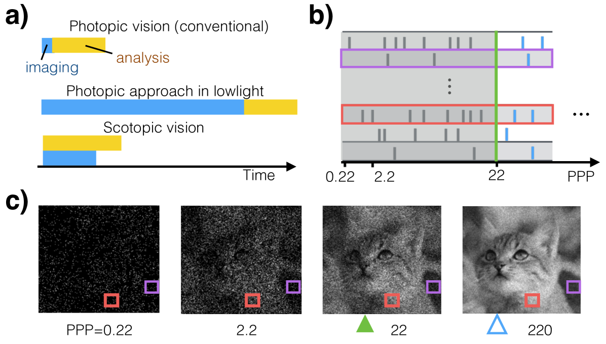
Consider now the opposite situation, which we call scotopic vision222The term ‘scotopic / photopic vision’ literally means ‘vision in the dark / with plenty of light’. It is usually associated to the physiological state where only rods, not cones, are active in the retina. We use ‘scotopic vision’ to denote the general situation where a visual system is starved for photons, regardless the technology used to capture the image., where photons are few and precious, and exposure time is long compared to computation time. The design tradeoff is between accuracy and exposure time [3], and computation time becomes a small additive constant.
Why worry about scotopic vision? We ask the opposite question: “Why waste time collecting unnecessary photons?” There are multiple situations where this question is compelling. (1) One may be trying to sense/control dynamics that are faster than the exposure time that guarantees good quality pictures, e.g. automobiles and quadcopters [4]. (2) In competitive scenarios, such as sports, a fraction of a second may make all the difference between defeat and victory [5]. (3) Sometimes prolonged imaging has negative consequences, e.g. because phototoxicity and bleaching alter a biological sample [6] or because of health risks in medical imaging [7]. (4) In sensor design, reduced photon counts allow for imaging with smaller pixels and ultra-high resolution [8, 9]. (5) sometimes there is little light in the environment, e.g. at night, and obtaining a good quality image takes a long time relative to achievable computational speed. Thus, it is compelling to understand how many photons are needed for good-enough vision, and how one can make visual decisions as soon as a sufficient number of photons has been collected. In scotopic vision photons are collected until the evidence is sufficient to make a decision.
Our work is further motivated by the recent development of photon-counting imaging sensors: single photon avalanche diode arrays [10], quanta image sensors [9], and gigavision cameras [8]. These sensors detect and report single photon arrival events in quick succession, an ability that provides fine-grained control over photon acquisition that is ideal for scotopic vision applications. By contrast, conventional cameras, which are designed to return a high-quality image after a fixed exposure time, produce an insurmountable amount of noise when forced to read out images rapidly and are suboptimal at low light. Current computer vision technology has not yet taken advantage of photon-counting sensors since they are still under development. Fortunately, realistic noise models of the sensors [9] are already available, making it possible (and wise) to innovate computational models that leverage and facilitate the sensor development.
While scotopic vision has been studied in the context of the physiology and technology of image sensing [11, 12], as well as the physiology and psychophysics of visual discrimination [13] and visual search [14], little is known regarding the computational principles for high-level visual tasks, such as categorization and detection, in scotopic settings. Prior work on photon-limited image classification [15] deals with a single image, and does not study the trade-off between exposure time and accuracy. Instead, our work explores scotopic visual categorization on modern datasets such as MNIST and CIFAR10 [16, 17], examines model performance under common sensory noise, and proposes realistic implementations of the algorithm.
Our main contributions are:
1. A computational framework for scotopic classification that can trade-off accuracy and response time.
2. A feedforward architecture yielding any-time, quasi-optimal scotopic classification.
3. A learning algorithm optimizing the speed accuracy tradeoff of lowlight classifiers.
4. Robustness analysis regarding sensor noise in current photon-counting sensors.
5. A spiking implementation that trades off accuracy with computation / power.
6. A light-level estimation capacity that allows the implementation to function without an external clock and at situations with unknown illuminance levels.
2 Previous Work
Our approach to scotopic visual classification is probabilistic. At every time instant each classification hypothesis is tested based on the available evidence. Is there sufficient evidence to make the decision? If so, then the pattern is classified. If not, the system will delay classification, acquire more photons, i.e. more information, and try again. This approach descends from Wald’s Sequential Probablistic Ratio Test (SPRT) [18]. Wald proved optimality of SPRT under fairly stringent conditions (see Sec. 3). Lorden, Tartakowski and collaborators [19, 20] later showed that SPRT is quasi-optimal in more general conditions, such as the competition of multiple one-sided tests, which turns out to be useful in multiclass visual classification.
Feedforward convolutional neural networks (ConvNets) [21] have been recently shown to be trainable to classify images with great accuracy [17, 22, 23]. We show that ConvNets are inadequate for scotopic vision. However, they are very appropriate once opportune modifications are applied. In particular, our scotopic algorithm marries ConvNet’s specialty for classifying good-quality images with SPRT’s ability to trade off photon acquisition time with classification accuracy in a near-optimal fashion.
Sequential testing has appeared in the computer vision literature [24, 25, 26] in order to shorten computation time. These algorithms assume that all visual information (‘the image’) is present at the beginning of computation, thus focus on reducing computation time in photopic vision. By contrast, our work aims to reduce capture time and is based on the assumption that computation time is negligible when compared to image capture time. In addition, these algorithms either require an computationally intensive numerical optimization [27] or fail to offer optimality guarantees [28, 29]. In comparison, our proposed strategy has a closed-form and is asymptotically optimal in theory.
Sequential reasoning has seen much recent success thanks to the use of recurrent neural networks (RNN) [30, 31]. Our work is inherently recurrent as every incoming photon prompts our system to update its decision, hence we exploits recurrence for efficient computation. Yet, conventional RNNs are trained with inputs that are sampled uniformly in time, which in our case would translate to photon counting images per second and would be highly inefficient. Instead, we employ a continuous-time RNN [32] approximation that can be trained using images sampled at arbitrary times, and find that a logarithmic number of () samples per sequence suffice in practice.
Scotopic vision has been studied by physiologists and psychologists. Traditionally their main interest is understanding the physiology of phototransduction and of local circuitry in the retina as well as the sensitivity of the human visual system at low light levels [33, 34, 35], thus there is no attempt to understand ‘high level’ vision in scotopic conditions. More recent work has begun addressing visual discrimination and search under time-pressure, such as phenomenological diffuse-to-threshold models [36] and Bayesian models of discrimination and of visual search [13, 37, 14]. The pictures used in these studies are the simple patterns (moving gratings and arrangements of oriented lines) that are used by visual psychophysicists. Our work is the first attempt to handle general realistic images.
Lastly, VLSI designers have produced circuits that can signal pixel ‘events’ asynchronously [38, 12, 39] as soon as a sufficient amount of signal is present. This is ideal for our work since conventional cameras acquire images synchronously (all pixels are shuttered and A-D converted at once) and are therefore ill-adapted to scotopic vision algorithms. The idea of event-based computing has been extended to visual computation by O’Connor et al. [40] who developed an event-based deep belief network that can classify handwritten digits. The classification algorithms and the spiking implementation that we propose are distantly related to this work. Our emphasis is to study the best strategies to minimize response time, while their emphasis is on spike-based computation.
3 A Framework for Scotopic Classification
3.1 Image Capture
Our computational framework starts from a model of image capture. Each pixel in an image reports the brightness estimate of a cone of visual space by counting photons coming from that direction. The estimate improves over time. Starting from a probabilistic assumption of the imaging process and of the target classification application, we derive an approach that allows for the best tradeoff between exposure time and classification accuracy.
We make three assumptions and relax them later:
- •
-
•
Photon arrival times follow a homogeneous Poisson process. This assumption is only used to develop the model. We will evaluate the model in Sec. 4.4 using observations from realistic noise sources.
-
•
A probabilistic classifier based on photon counts is available. We discuss how to obtain such a model in Sec. 3.4.
Formally, the input is a stream of photons incident on the sensors during time , where time has been discretized into bins of length . is the number of photons arrived at pixel in the th time interval, i.e. . The task of a scotopic visual recognition system is two fold: 1) computing the category of the underlying object, and 2) crucially, determining and minimizing the exposure time at which the observations are deemed sufficient.
3.1.1 Noise Sources
The pixels in the image are corrupted by several noise sources intrinsic to the camera [41]. Shot noise: The number of photons incident on a pixel in the unit time follows a Poisson distribution whose rate (Hz) depends on both the pixel intensity and a dark current :
| (1) |
where is the illuminance (maximum photon count per pixel) per unit time [1, 8, 41, 42]. During readout, the photon count is additionally corrupted first by the amplifier’s read noise, which is an additive Gaussian, then by the fixed-pattern noise which may be thought of as a multiplicative Gaussian noise [43]. As photon-counting sensors are designed to have low read noise and low fixed pattern noise[9, 10, 42], we focus on modeling the shot noise and dark current only. We will show (Sec. 4.4) that our models are robust against all four noise sources. Additionally, according to the stationary assumption there is no motion-induced blur. For simplicity we do not model charge bleeding and cross-talk in colored images, and assume that they will be mitigated by the sensor community [44].
When the illuminance of the environment is fixed, the average number of photons per pixel (PPP)333PPP is averaged across the entire scene and duration. is linear in :
| (2) |
hence we will use time and PPP interchangeably. Since the information content in the image is directly related to the amount of photons, from now on we measure response time in terms of PPP instead of exposure time. Fig. 1 shows a series of images with increasing PPP. See Sec. 3.5 for cases where the illuminance is varying in time.
3.2 Sequential probability ratio test
Our decision strategy for trading off accuracy and speed is based on SPRT, for its simplicity and attractive optimality guarantees. Assume that a probabilistic model is available to predict the class label given a sensory input of any duration – either provided by the application or learned from labeled data using techniques described in Sec. 3.4 – SPRT conducts a simple accumulation-to-threshold procedure to estimate the category :
Let denote the class posterior probability ratio of the visual category for photon count input , , and let be an appropriately chosen threshold. SPRT conducts a simple accumulation-to-threshold procedure to estimate the category :
| Compute | ||||
| (3) |
When a decision is made, the declared class has a probability that is at least times bigger thanthe probability of all the other classes combined, therefore the error rate of SPRT is at most , where is the sigmoid function: .
For simple binary classification problems, SPRT is optimal in trading off speed versus accuracy in that no other algorithm can respond faster while achieving the same accuracy [18]. In the more realistic case where the categories are rich in intra-class variations, SPRT is shown to be asymptotically optimal, i.e. it gives optimal error rates as the exposure time becomes large [19]. Empirical studies suggest that even for short exposure times SPRT is near-optimal [45].
In essence, SPRT decides when to respond dynamically, based on the stream of observations accumulated so far. Therefore, the response time is different for each example. This regime is called “free-response” (FR), in contrast to the “interrogation” (INT) regime, typical of photopic vision, where a fixed-length observation is collected for each trial [46]. The observation length may be chosen according to a training set and fixed a priori. In both regimes, the length of observation should take into account the cost of errors, the cost of time, and the difficulty of the classification task.
Despite the striking similarity between the two regimes, SPRT (the FR regime) is provably optimal in the asymptotical tradeoff between response time and error rate, while such proofs do not exist for the INT regime. We will empirically evaluate both regimes in Sec. 4.3.3.
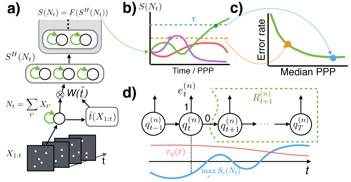
3.3 Computing class probabilities over time
The challenge of applying SPRT is to compute for class and the input stream of variable exposure time , or in a more information-relevant unit, variable PPP levels. Thanks to the Poisson noise model (Eq. 1), the sufficient statistics for observation is the cumulative count (visualized in Fig. 1), and the observation duration length , therefore we may rewrite as . We further shorthand the notation to since the exposure time is evident from the subscript. Since counts at different PPPs (and, equivalently, exposure times) have different statistics, it would appear that a specialized system is required for each PPP. This leads to the naive ensemble approach. Instead, we also propose a network called WaldNet that can process images at all PPPs and has the size of only a single specialized system. We describe the two approaches below.
3.3.1 Model-free approach: network ensembles
The simple idea is to build a separate ‘specialist’ model for each exposure time (or light level PPP), either based on domain knowledge or learned from a training set. For best results one needs to select a list of representative light levels to train the specialists, and route input counts to the specialist closest in light level. We refer to this as the ‘ensemble’ predictor.
One potential drawback of this ensemble approach is that training and storing multiple specialists is wasteful. At different light levels, while the cumulative counts change drastically, the underlying statistical structure of the task stays the same. An approach that takes advantage of this relationship may lead to more parsimonious algorithms.
3.3.2 Model-based approach: WaldNet
Unlike the ensemble approach, we show that one can exploit the structure of the input and build one system for images at all PPPs. The variation in the input has two independent sources: one is the stochasticity in the photon arrival times, and the other the intra- and inter- class variation of the real intensity values of the object. SPRT excels at reasoning about the first noise source while deep networks are ideal for capturing the second. Therefore we propose WaldNet, a deep network for speed-accuracy tradeoff (Fig. 2b-c) that combines ConvNets with SPRT. WaldNet automatically adjusts the parameters of a ConvNet according to the exposure time . Thus a WaldNet may be viewed as an ensemble of infinitely many specialists that occupies the size of only one specialist.
The key ingredient to SPRT is the log posterior ratios over exposure time . Standard techniques such as ConvNets can not be applied directly as their input is static, namely the cumulative photon counts up to an identical exposure time (e.g. in normal lighting conditions). However we propose a simple adjustment that transfers the uncertainty in the photon counts to uncertainty in the task-relevant features of a ConvNet.
A standard ConvNet contains multiple layers of computations that may be viewed as a nesting of two transformations: (1) the first hidden layer that maps the input to a feature vector444Without loss of generality and for notational simplicity, we assume that the first layer is fully-connected as oppose to convolutional. Sec. 0.A.1 discusses how to extend the results here to convolutional layers. We also define the first layer feature as the activity prior to non-linearity., and (2) the remaining layers that map the features to the log class posterior probabilities . is a weight vector and is a bias vector.
Given only partial observations , computing features of the first layer requires marginalizing out unobserved photon counts . The marginalization requires putting a prior on the photon emission rate per image pixel , which we assume to be a Gamma distribution: , where represents the prior mean rate for pixel and (shared across pixels) represents the strength of the prior555We use a Gamma prior because it is the conjugate prior of the Poisson likelihood.. Then the first layer of hidden features may be approximated by:
| (4) |
where the scaling factor is a scalar and the biases is a length vector. For the -th hidden feature, . Detailed derivations are in Sec. 0.A.1.
Essentially, the adaptation procedure in Eq. 4 accounts for the stochasticity in photon arrival time by using time-dependent weights and biases, rendering an exposure-time invariant feature representation . The computations downstream, , may then treat as if it were obtained from the entire duration. Therefore the same computations suffice to model the intra- and inter-class variations: .
The network is trained discriminately (Sec. 3.4) with the first layer replaced by Eq. 4. The network has nearly the same number of parameters as a conventional ConvNet, but has the capacity to process inputs at different exposure times. The adaptation is critical for performance, as will be seen by comparison with simple rate-based methods in Sec. 4. See Sec. 4.2.2 for implementation details.
3.4 Learning
Our goal is to train WaldNet to optimally trade off the expected exposure time (or PPP) and error rate in the FR regime. Optimality is defined by the Bayes risk [18]:
| (5) |
where [PPP] is the expected photon count required for classification, is the error rate, and describes the user’s cost of photons per pixel (PPP) versus error rate. WaldNet asymptotically optimizes the Bayes risk provided that it can faithfully capture the class log posterior ratio , and selects the correct threshold (Eq. 3) based on the tradeoff parameter . Sweeping traverses the optimal time versus error tradeoff (Fig. 2c).
Since picking the optimal threshold according to is independent from training a ConvNet to approximately compute the log posterior ratio , the same ConvNet is shared across multiple ’s. This suggests the following two-step learning algorithm.
3.4.1 Step one: posterior learning
Given a dataset where indexes training examples and indexes exposure time, we train the adapted ConvNet to minimize:
| (6) |
where collectively denote all the parameters in the adapted ConvNet, and denotes weight-decay on the filters. When a lowlight dataset is not available we simulate the dataset from normal images according to the noise model in Eq. 1, where the exposure times are sampled uniformly on a logarithmic scale (see Sec. 4).
3.4.2 Step two: threshold tuning
If the ConvNet in step one captures the log posterior ratio , we can simply optimize a scalar threshold for each tradeoff parameter . In practice, we may opt for a time-varying threshold as step one may not be perfect666For instance, consider an adapted ConvNet that perfectly captures the class posterior. Ignoring the regularizer (right term of Eq. 6), we can scale up the weights and biases of the last layer (softmax) by an arbitrary amount without affecting the error rate, which scales the negative log likelihood (left term in Eq. 6) by a similar amount, leading to a better objective value. The magnitude of the weights are thus determined by the regularizer and may be off by a scaling factor. We therefore need to properly rescale the class posterior at every exposure time before comparing to a constant threshold, which is equivalent to using a time-varying threshold on the raw predictions..
affects our Bayes risk objective in the following way (Fig. 2d). Consider a high-quality image , let be a sequence of lowlight images increasing in PPP generated from . Denote the event that the log posterior ratio crosses decision threshold at time , and the event that the class prediction at is wrong. Let denote the Bayes risk of the sequence incurred from time onwards. may be computed recursively (derived in Sec. 0.A.2):
| (7) |
where the first term is the cost of collecting photons at time , the second term is the expected cost of committing to a decision that is wrong, and the last term is the expected cost of deferring the decision till more photons are collected.
The Bayes risk is obtained from averaging multiple photon count sequences, i.e. . is non-differentiable with respect to the threshold , leading to difficulties in optimizing . Instead, we approximate with a Sigmoid function:
| (8) |
where , and anneal the temperature of the Sigmoid over the course of training [47] (see Sec. 4).
3.5 Automatic light-level estimation
Both scotopic algorithms (ensemble and WaldNet) assume knowledge of the light-level PPP in order to choose the right model parameters. This knowledge is easy to acquire when the illuminance is constant over time, in which case PPP is linear in the exposure time (Eq. 2), which may be measured by an internal clock.
However, in situations where the illuminance is dynamic and unknown, the linear relationship between PPP and exposure time is lost. In this case we propose to estimate PPP directly from the photon stream itself, as follows. Given a cumulative photon count image (, the time it takes to accumulate the photons, is no longer relevant as the illuminance is unknown), we examine local neighbors that receive high photon counts, and pool the photon counts as a proxy for PPP. In detail, we (1) convolve using an box filter, (2) compute the median of the top responses, and (3) fit a second order polynomial to regress the median response towards the true PPP. Here and are parameters, which are learned from a training set consisting of PPP pairs. Despite its simplicity, this estimation procedure works well in practice, as we will see in Sec. 4.
3.6 Spiking implementation
One major challenge of scotopic systems is to compute log posterior ratio computations as quickly as photons stream in. Photon-counting sensors [8, 9] sample the world at , while the fastest reported throughput of ConvNet [48] is for color images, and for color images. Fortunately, the reported throughputs are based on independent images, whereas the scotopic systems operate on photon streams, where temporal coherence may be leveraged for accelerated processing. Since the photon arrival events within any time bin is sparse, changes to the input and the internal states of a scotopic system are small. An efficient implementation thus could model the changes and propagate only those that are above a certain magnitude.
One such implementation relies on spiking recurrent hidden units. A spiking recurrent hidden unit is characterized by two aspects: 1) computation at time reuses the unit’s state at time and 2) only changes above a certain level will be propagated to layers above.
Specifically, the first hidden layer of WaldNet may be exactly implemented using the following recurrent network where the features (Eq. 4) are represented by membrane voltages . The dynamics of is:
| (9) |
where is a damping factor, is a leakage term (derivations in Sec. 0.A.3). The photon counts in is sparse, thus the computation is more efficient than computing from scratch.
To propagate only large changes to the layers above, we use a similar thresholding mechanism as (Eq. 3). For each hidden unit , we associate a ‘positive’ and a ’negative’ neuron that communicate with the layer above. For each time bin :
| (10) |
where is a discretization threshold. By taking the difference between the spike counts from the ‘positive’ and the ‘negative’ neuron, the layers above can reconstruct a discretized version of . Hidden units from higher layers in WaldNet may be approximated using spiking recurrent units (Eq. 9) in a similar fashion.
The discretization threshold affects not only the number of communication spikes, but also the quality of the discretization, and in turn the classification accuracy. For spike-based hardwares [49], the number of spikes is an indirect measure of the energy consumption (Fig. 4(B) of [49]). For non-spiking hardwares, the number of spikes also translate to the number of floating point multiplications required for the layers above. Therefore, the controls the tradeoff between accuracy and power / computational cost. We will empirically evaluate this tradeoff in Sec. 4.
4 Experiments
4.0.1 Exposure time versus signal
Our experiments use PPP interchangeably with exposure time for performance measurement, since PPP directly relates to the number of bits of signal in each pixel. In practice an application may be more concerned with exposure time. Thus it is helpful to relate exposure time with the bits of signal. Table 1 describes this relationship for different illuminance levels (see Sec. 0.A.4 for derivations).
| Illuminance | exposure time (s) | ||||||
| Scene | Ev (LUX) | 1/500 | 1/128 | 1/8 | 1 | 8 | 60 |
| Moonless | 1.5 | 3 | |||||
| Full moon | 0.5 | 1.5 | 3.5 | 5 | 6.5 | 8 | |
| Office | 4.5 | 5.5 | 7.5 | 9 | 10.5 | 12 | |
| Overcast | 5.5 | 6.5 | 8.5 | 10 | 11.5 | 13 | |
| Bright sun | 9 | 10 | 12 | 13.5 | 15 | 16.5 | |
4.1 Baseline Models
We compare WaldNet against the following baselines, under both the INT regime and the FR regime:
Ensemble. We construct an ensemble of specialists with PPPs from respectively. The performance of the specialists at their respective PPPs gives a lower bound on the optimal performance by ConvNets of the same architecture.
Photopic classifier. An intuitive idea is to take a network trained in normal lighting conditions, and apply it to properly rescaled lowlight images. We choose the specialist with PPP as the photopic classifier as it achieves the same accuracy as a network trained with -bit images.
Rate classifier. A ConvNet on the time-normalized image (rate) without weight adaptation. The first hidden layer is computed as . Note the similarity with the WaldNet approximation used in Eq. 4.
For all models above we assume that an internal clock measures the exposure time , and the illuminance is known and constant over time. We remove this assumption for the model below for unknown and varying illuminance:
WaldNet with estimated light-levels. A WaldNet that is trained on constant illuminance , but tested in environments with unknown and dynamic illuminance. In this case the linear relationship between exposure time and PPP (Sec. 2) is lost. Instead, the light-level is first estimated according to Sec. 3.5 directly from the photon count image . The estimate is then converted to an ‘equivalent’ exposure time using (by inverting Eq. 2), which is used to adapt the first hidden layer of WaldNet in Sec. 4, i.e. .
4.2 Datasets
We consider two standard datasets: MNIST [17] and CIFAR10 [16]. We simulate lowlight image sequences using Eq. 1.
MNIST contains gray-scaled images of hand-written digits. It has training and test images. We treat the pixel values as the ground truth intensity777The brightest image we synthesize has about photons, which corresponds to a pixel-wise maximum signal-to-noise ratio of (-bit accuracy), whereas the original MNIST images has ( to -bit accuracy) that corresponds to to photons. . Dark current . We use the default LeNet architecture from the MatConvNet package [50] with batch normalization [51] after each convolution layer. The architecture is ----888The first and last number represent the input and output dimension, each number in between represents the number of feature maps used for that layer. The number of units is the product of the number of features maps with the size of the input. with receptive fields and pooling.
CIFAR10 contains color images of visual categories. It has training and test images. We use the same sythensis procedure above to each color channel999For simplicity we do not model the Bayer filter mosaic.. We again use the default ---- LeNet architecture [22] with batch normalization. We use the same setting prescribed in [22] to achieve test error on normal lighting conditions. [22] uses local contrast normalization and ZCA whitening as preprocessing steps. We estimate the local contrast and ZCA from normal lighting images and transforming them according to the lowlight model to preprocess scotopic images.
4.2.1 Training
We train all models for MNIST and CIFAR10 using stochastic gradient descent with mini-batches of size . For MNIST, we use training examples for validation and train on the remaining examples for iterations. We found that empirically a learning rate of works best for WaldNet, and works best for the other architectures. As CIFAR10 is relatively data-limited, we do not use a validate set and instead train all models for epochs, where the learning rate is for iterations, for other then for the rest. Again, quadrupling the learning rate empirically improves WaldNet’s performance but not the other architectures.
4.2.2 Implementation of WaldNet
Our implementation is based on MatCovNet [50], and publicly available101010https://github.com/bochencaltech/scotopic.
In step one of learning, the scalar functions and in Eq. 4 are learned as follows. As the inputs to the network are preprocessed, the preprocessing steps alter the algebraic form for and . For flexibility we do not impose parametric forms on and , but represent them with piecewise cubic Hermite interpolating polynomials with four end points at PPP (interpolants coded in log-scale). We learned the adapted weights at these end-points by using a different batch normalization module for each PPP. At test time the parameters of the modules are interpolated to accommodate other PPP levels.
In step two of learning, we compute for uniformly spaced PPPs in log scale, and train thresholds for each PPP and for each . A regularizer is imposed on the thresholds to enforce smoothness. In Eq. 8, the steepness of Sigmoid is annealed over iterations of gradient descent, with initial value , a decay rate of and a floor value of .
4.3 Results
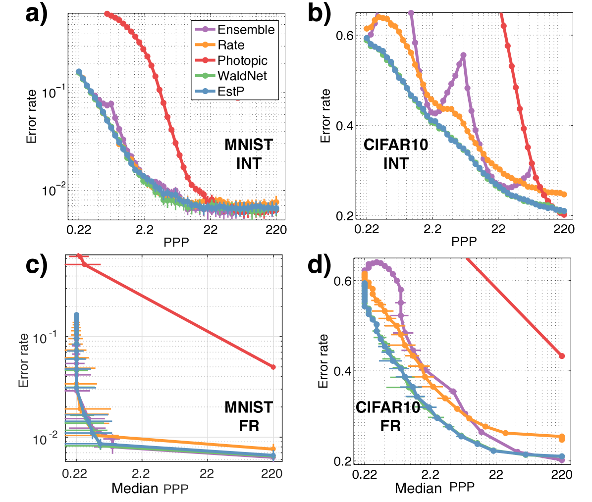
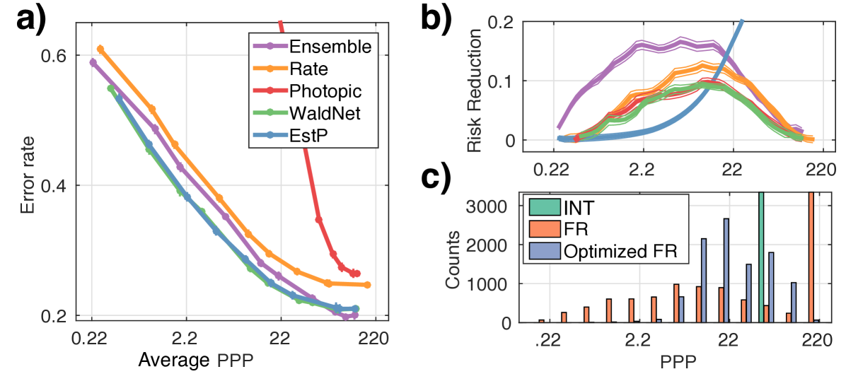
The speed versus accuracy tradeoff curves in the INT regime are shown in Fig. 3a,b. Median PPP versus accuracy tradeoffs for all models in the FR regime are shown in Fig. 3c,d. All models use constant thresholds for producing the tradeoff curves. In Fig. 4a are average PPP versus accuracy curves when the models use optimized dynamic thresholds described in Sec. 3.4, step-two.
4.3.1 Model comparisons
Overall, WaldNet performs well under lowlight. It only requires PPP to stay within (absolute) degradation in accuracy on MNIST and around PPP to stay within degradation on CIFAR10.
WaldNet is sufficient. The ensemble was formed using specialists at logarithmically-spaced exposure times, thus its curve is discontinuous in the interrogation regime (esp. Fig. 3b). The peaks delineate transitions between specialists. The ensemble’s performance at the specialized light levels also provides a proxy for the performance upper bound by ConvNets of the same architecture (apart from overfitting and convergence issues during learning). Using this proxy we see that even though WaldNet uses the parameters of the ensemble, it stays close to the performance upper bound. Under the FR regime, WaldNet is indistinguishable from the ensemble in MNIST and superior to the ensemble in lowlight conditions ( PPP, perhaps due to overfitting) of CIFAR10. This showcases WaldNet’s ability to handle images at multiple PPPs without requiring explicit parameters.
Training with scotopic images is necessary. The photopic classifier retrofitted to lowlight applications performs well at high light conditions ( PPP) but works poorly overall in both datasets. Investigation reveals that the classifier often stops evidence collection prematurely. This shows that despite effective learning, training with scotopic images and having the proper stopping criterion remain crucial.
Weight adaptation is necessary. The rate classifier slightly underperforms WaldNet in both datasets. Since the two system have the same degrees of freedom and differ only in how the first layer feature is computed, the comparison highlights the advantage of adopting time-varying features (Eq. 4).
4.3.2 Effect of threshold learning
The comparison above under the FR regime uses constant thresholds on the learned log posterior ratios (Fig. 3c,d). Using learned dynamic thresholds (step two of Sec. 3.4) we see consistent improvement on the average PPP required for given error rate across all models (Fig. 4b), with more benefit for the photopic classifier. Fig. 4c examines the PPP histograms on CIFAR10 with constant (FR) versus dynamic threshold (optimized FR). We see with constant thresholds many decisions are made at the PPP cutoff of , so the median and the mean are vastly different. Learning dynamic thresholds reduces the variance of the PPP but make the median longer. This is ok because the Bayes risk objective (Eq. 5) concerns the average PPP, not the median. Clearly which threshold to use depending on whether the median or the mean is more important to the application.
4.3.3 Effect of interrogation versus free-response
4.4 Sensitivity to sensor noise
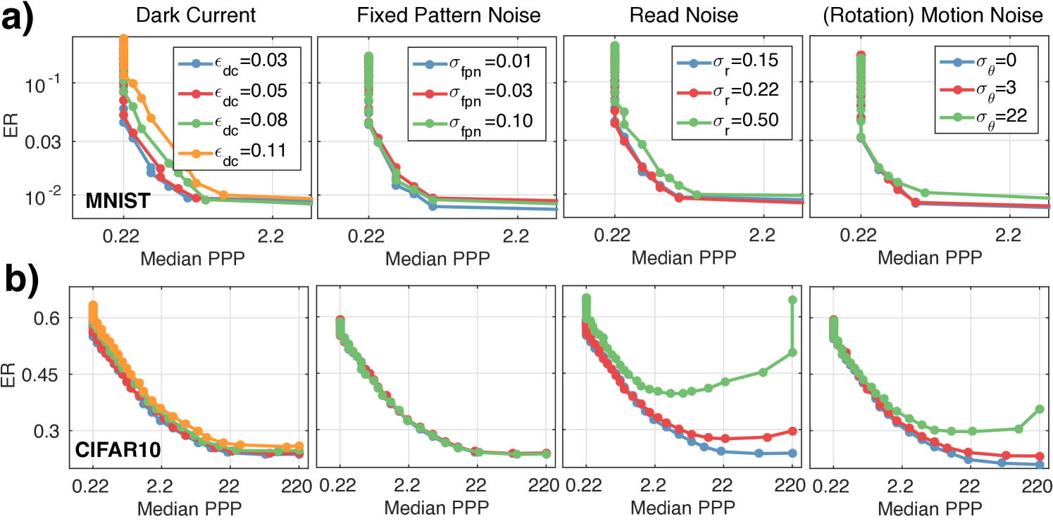
How robust is the speedup observed in Sec. 4.3 affected by sensor noise? For MNIST and CIFAR10, we take WaldNet and vary independently the dark current, the read noise and the fixed pattern noise. We also introduce a rotational jitter noise to investigate the model’s robustness to motion. The jitter applies a random rotation to the camera (or equivalently to the object being imaged by a stationary camera) where the rotation at PPP follows a normal distribution: , where controls the level of jitter. e.g. means that at , the total amount of rotation applied to the image has an std of . The result is shown in Fig. 5a,b.
First, the effect of dark current and fixed pattern noise is minimal. Even an dark current (i.e. photon emission rate of the darkest pixel is of that of the brightest pixel) merely doubles the exposure time with little loss in accuracy. The multiplicative fixed pattern noise does not affect performance because WaldNet in general makes use of very few photons. Second, current industry standard of read noise ( [9]) guarantees no performance loss for MNIST and minor loss for CIFAR10, suggesting the need for improvement in both the algorithm and the photon-counting sensors. The fact that hurts performance also suggests that single-photon resolution is vital for scotopic vision. Lastly, while WaldNet provides certain tolerance to rotational jitter, drastic movement ( at PPP) could cause significant drop in performance, suggesting that future scotopic recognition systems and photon-counting sensors should not ignore camera / object motion.
4.5 Efficiency of spiking implementation
Finally, we inspect the power efficiency of the spiking network implementation (Eq. 9, 10) on the MNIST dataset. Our baseline implementation (“Continuous”) runs a ConvNet from end-to-end every time the input is refreshed. As a proxy for power efficiency we use the number of multiplications [49], normalized by the total number in the baseline. For simplicity we vary the discretization threshold for inducing spiking events (Eq. 10), and the threshold is common across all layers.
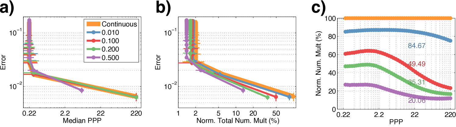
The power, speed and accuracy results shown in Fig. 6a,b suggest that for discretization not only faithfully preserves the SAT of WaldNet (Fig. 6a), but also could be optimized to consume only of the total multiplications, i.e. the spiking implementation provides a power reducation. The amount of spiking events starts high and tappers off gradually (Fig. 6c) as the noise in the hidden unit estimates (Eq. 9) improves over time. Thus most of the computational savings comes at the later stage (). Further savings may reside in optimizing the discretization thresholds per layer or over time, which we reserve for future investigations.
5 Discussion and Conclusions
We proposed to study the important yet relatively unexplored problem of scotopic visual recognition. Scotopic vision is vision starved for photons. This happens when available light is low, and image capture time is longer than computation time. In this regime vision computations should start as soon as the shutter is opened, and algorithms should be designed to process photons as soon as they hit the photoreceptors. While visual recognition from limited evidence has been studied [52], to our knowledge, our study is the first to explore the exposure time versus accuracy trade-off of visual classification, which is essential in scotopic vision.
We proposed WaldNet, a model that combines photon arrival events over time to form a coherent probabilistic interpretation, and make a decision as soon as sufficient evidence has been collected. The proposed algorithm may be implemented by a deep feed-forward network similar to a convolutional network. Despite the similarity of architectures, we see clear advantages of approaches developed specifically for the scotopic environment. An experimental comparison between WaldNet and models of the conventional kind, such as photopic approaches retrofitted to lowlight images and ensemble-based approaches agnostic of lowlight image statistics, shows large performance differences, both in terms of model parsimony and response time (measured by the amount of photons required for decision at desired accuracy). WaldNet further allows for a flexible tradeoff between power / computational efficiency with accuracy when implemented as a recurrent spiking network. When trained assuming a constant illuminance, WaldNet may be applied in environments with varying and unknown illuminance levels. Finally, despite relying only on few photons for decisions, WaldNet is minimally affected by camera noises, making it an ideal model to be integrated with the evolving lowlight sensors.
References
- [1] Morris, P.A., Aspden, R.S., Bell, J.E., Boyd, R.W., Padgett, M.J.: Imaging with a small number of photons. Nature communications 6 (2015)
- [2] Dollar, P., Appel, R., Belongie, S., Perona, P.: Fast feature pyramids for object detection. Submitted to IEEE Trans. on Pattern Anal. and Machine Intell. (2013)
- [3] Ferree, C., Rand, G.: Intensity of light and speed of vision: I. Journal of Experimental Psychology 12(5) (1929) 363
- [4] Dickmanns, E.D.: Dynamic vision for perception and control of motion. Springer Science & Business Media (2007)
- [5] Thorpe, S., Fize, D., Marlot, C., et al.: Speed of processing in the human visual system. nature 381(6582) (1996) 520–522
- [6] Stephens, D.J., Allan, V.J.: Light microscopy techniques for live cell imaging. Science 300(5616) (2003) 82–86
- [7] Hall, E., Brenner, D.: Cancer risks from diagnostic radiology. Cancer 81(965) (2014)
- [8] Sbaiz, L., Yang, F., Charbon, E., Süsstrunk, S., Vetterli, M.: The gigavision camera. In: Acoustics, Speech and Signal Processing, 2009. ICASSP 2009. IEEE International Conference on, IEEE (2009) 1093–1096
- [9] Fossum, E.: The quanta image sensor (qis): concepts and challenges. In: Imaging Systems and Applications, Optical Society of America (2011) JTuE1
- [10] Zappa, F., Tisa, S., Tosi, A., Cova, S.: Principles and features of single-photon avalanche diode arrays. Sensors and Actuators A: Physical 140(1) (2007) 103–112
- [11] Barlow, H.: A method of determining the overall quantum efficiency of visual discriminations. The Journal of physiology 160(1) (1962) 155–168
- [12] Delbrück, T., Mead, C.: Analog vlsi phototransduction. Signal 10(3) (1994) 10
- [13] Gold, J.I., Shadlen, M.N.: Banburismus and the brain: decoding the relationship between sensory stimuli, decisions, and reward. Neuron 36(2) (Oct 2002) 299–308
- [14] Chen, B., Navalpakkam, V., Perona, P.: Predicting response time and error rate in visual search. In: Neural Information Processing Systems (NIPS). (Granada, 2011)
- [15] Wernick, M.N., Morris, G.M.: Image classification at low light levels. JOSA A 3(12) (1986) 2179–2187
- [16] Krizhevsky, A., Hinton, G.: Learning multiple layers of features from tiny images (2009)
- [17] LeCun, Y., Bottou, L., Bengio, Y., Haffner, P.: Gradient-based learning applied to document recognition. Proceedings of the IEEE 86(11) (1998) 2278–2324
- [18] Wald, A.: Sequential tests of statistical hypotheses. The Annals of Mathematical Statistics 16(2) (1945) 117–186
- [19] Lorden, G.: Nearly-optimal sequential tests for finitely many parameter values. The Annals of Statistics (1977) 1–21
- [20] Tartakovsky, A.G.: Asymptotic optimality of certain multihypothesis sequential tests: Non-iid case. Statistical Inference for Stochastic Processes 1(3) (1998) 265–295
- [21] Fukushima, K.: Neocognitron: A self-organizing neural network model for a mechanism of pattern recognition unaffected by shift in position. Biological cybernetics 36(4) (1980) 193–202
- [22] Krizhevsky, A., Sutskever, I., Hinton, G.: Imagenet classification with deep convolutional neural networks. In: Advances in Neural Information Processing Systems 25. (2012) 1106–1114
- [23] Jia, Y., Shelhamer, E., Donahue, J., Karayev, S., Long, J., Girshick, R., Guadarrama, S., Darrell, T.: Caffe: Convolutional architecture for fast feature embedding. arXiv preprint arXiv:1408.5093 (2014)
- [24] Viola, P., Jones, M.: Rapid object detection using a boosted cascade of simple features. In: Computer Vision and Pattern Recognition, 2001. CVPR 2001. Proceedings of the 2001 IEEE Computer Society Conference on. Volume 1., IEEE (2001) I–511
- [25] Moreels, P., Maire, M., Perona, P.: Recognition by probabilistic hypothesis construction. In: Computer Vision-ECCV 2004. Springer (2004) 55–68
- [26] Matas, J., Chum, O.: Randomized ransac with sequential probability ratio test. In: Computer Vision, 2005. ICCV 2005. Tenth IEEE International Conference on. Volume 2., IEEE (2005) 1727–1732
- [27] Naghshvar, M., Javidi, T., et al.: Active sequential hypothesis testing. The Annals of Statistics 41(6) (2013) 2703–2738
- [28] Zhu, M., Atanasov, N., Pappas, G.J., Daniilidis, K.: Active deformable part models inference. In: European Conference on Computer Vision, Springer (2014) 281–296
- [29] Chen, B., Perona, P., Bourdev, L.D.: Hierarchical cascade of classifiers for efficient poselet evaluation. In: BMVC. (2014)
- [30] Hochreiter, S., Schmidhuber, J.: Long short-term memory. Neural computation 9(8) (1997) 1735–1780
- [31] Graves, A., Liwicki, M., Fernández, S., Bertolami, R., Bunke, H., Schmidhuber, J.: A novel connectionist system for unconstrained handwriting recognition. IEEE transactions on pattern analysis and machine intelligence 31(5) (2009) 855–868
- [32] Li, X.D., Ho, J.K., Chow, T.W.: Approximation of dynamical time-variant systems by continuous-time recurrent neural networks. IEEE Transactions on Circuits and Systems II: Express Briefs 52(10) (2005) 656–660
- [33] Westheimer, G.: Spatial interaction in the human retina during scotopic vision. The Journal of physiology 181(4) (1965) 881–894
- [34] Frumkes, T.E., Sekuler, M.D., Reiss, E.H.: Rod-cone interaction in human scotopic vision. Science 175(4024) (1972) 913–914
- [35] Atick, J.J., Redlich, A.N.: What does the retina know about natural scenes? Neural computation 4(2) (1992) 196–210
- [36] Ratcliff, R.: Theoretical interpretations of the speed and accuracy of positive and negative responses. Psychological Review 92(2) (1985) 212
- [37] Drugowitsch, J., Moreno-Bote, R., Churchland, A., Shadlen, M., Pouget, A.: The cost of accumulating evidence in perceptual decision making. The Journal of Neuroscience 32(11) (2012) 3612–3628
- [38] Delbruck, T.: Silicon retina with correlation-based, velocity-tuned pixels. Neural Networks, IEEE Transactions on 4(3) (1993) 529–541
- [39] Liu, S.C., Delbruck, T., Indiveri, G., Whatley, A., Douglas, R.: Event-based Neuromorphic Systems. John Wiley & Sons (2014)
- [40] O’Connor, P., Neil, D., Liu, S.C., Delbruck, T., Pfeiffer, M.: Real-time classification and sensor fusion with a spiking deep belief network. Frontiers in neuroscience 7 (2013)
- [41] Liu, C., Szeliski, R., Kang, S.B., Zitnick, C.L., Freeman, W.T.: Automatic estimation and removal of noise from a single image. Pattern Analysis and Machine Intelligence, IEEE Transactions on 30(2) (2008) 299–314
- [42] Fossum, E.R.: Modeling the performance of single-bit and multi-bit quanta image sensors. Electron Devices Society, IEEE Journal of the 1(9) (2013) 166–174
- [43] Healey, G.E., Kondepudy, R.: Radiometric ccd camera calibration and noise estimation. Pattern Analysis and Machine Intelligence, IEEE Transactions on 16(3) (1994) 267–276
- [44] Anzagira, L., Fossum, E.R.: Color filter array patterns for small-pixel image sensors with substantial cross talk. JOSA A 32(1) (2015) 28–34
- [45] Chen, B., Perona, P.: Towards an optimal decision strategy of visual search. arXiv preprint arXiv:1411.1190 (2014)
- [46] Bogacz, R., Brown, E., Moehlis, J., Holmes, P., Cohen, J.D.: The physics of optimal decision making: a formal analysis of models of performance in two-alternative forced-choice tasks. Psychological review 113(4) (2006) 700
- [47] Mobahi, H., Fisher III, J.W.: On the link between gaussian homotopy continuation and convex envelopes. In: Energy Minimization Methods in Computer Vision and Pattern Recognition, Springer (2015) 43–56
- [48] Ovtcharov, K., Ruwase, O., Kim, J.Y., Fowers, J., Strauss, K., Chung, E.S.: Accelerating deep convolutional neural networks using specialized hardware. Microsoft Research Whitepaper 2 (2015)
- [49] Merolla, P.A., Arthur, J.V., Alvarez-Icaza, R., Cassidy, A.S., Sawada, J., Akopyan, F., Jackson, B.L., Imam, N., Guo, C., Nakamura, Y., et al.: A million spiking-neuron integrated circuit with a scalable communication network and interface. Science 345(6197) (2014) 668–673
- [50] Vedaldi, A., Lenc, K.: Matconvnet – convolutional neural networks for matlab. (2015)
- [51] Sergey Ioffe, C.S.: Batch normalization: Accelerating deep network training by reducing internal covariate shift. Volume 32. (2015) 448–456
- [52] Crouzet, S.M., Kirchner, H., Thorpe, S.J.: Fast saccades toward faces: face detection in just 100 ms. Journal of vision 10(4) (2010) 16
Appendix 0.A Appendix
0.A.1 Time-Adaptation of Hidden Features (Eq. 4)
Here we derive the approximation of the first layer activations given photon count image up to time (Eq. 4), copied as below:
| (0.A.1) |
Recall that we put a Gamma prior on the photon emission rate at pixel :
| (0.A.2) |
where is the prior mean rate at pixel .
After observing of pixel in time , the posterior estimate for the photon emission rate is:
| (0.A.3) | ||||
| (0.A.4) |
which has a posterior mean of:
| (0.A.5) |
Intuitively, the emission rate is estimated via a smoothed-average of the observed counts. Collectively the expected photon counts over all pixels and duration given the observed photons are:
| (0.A.6) |
where is the mean rate vector of all pixels.
Therefore may be approximated up to second order accuracy using:
| (0.A.7) | ||||
| (0.A.8) | ||||
| (0.A.9) | ||||
| (0.A.10) |
which proves Eq. 4.
The equation above works for weights that span the entire image. In ConvNet, the weights are instead localized (e.g. occupying only a region), and organized into groups (e.g. the first layer in WaldNet for CIFAR10 uses features groups). For simplicity we assume that the mean image is translational invariant within regions, so that we only need to model one scalar for each feature map .
0.A.2 Learning dynamic threshold for Bayes risk minimiziation (Eq. 7)
Here we show how thresholds relate to Bayes risk (Eq. 5) in the free-response regime with a cost of time . The key is to compute , the cumulative future risk from time for the -th example with label . At every point in time, the classifier first incurs a cost (assuming time unit of ) in collecting photons for this time point. Then the classifier either report a result according to , incurring a lost when the predicted label is wrong, or decides to postpone the decision till later, incurring lost . Which one of the two paths to take is determined by whether the max log posterior crosses the dynamic threshold . Therefore, let be the class with the maximum log posterior, the recursion is:
| (0.A.11) | ||||
| (0.A.12) |
and we assume that a decision must be taken after finite amount of time, i.e. . This proves Eq. 7.
0.A.3 Spiking recurrent neural network implementation
Here we show that the recurrent dynamics described in Eq. 9 implements the approximation of the first hidden layer activations in Eq. 4. The proof is constructive: assume that at time , the membrane potential computes , i.e. , then the membrane potential at time satisfies:
| (0.A.13) | ||||
| (0.A.14) | ||||
| (0.A.15) | ||||
| (0.A.16) |
Hence proving Eq. 9.
0.A.4 Relationship between exposure time and number of bits of signal (Table 1)
Bits of signal and photon counts are equivalent concepts. Furthermore, that photon counts are linearly related to exposure time. Here to derive the relationship between exposure time and the number of bits of signal. To simplify the analysis we will make the assumption that our imaging setup has a constant aperture.
What does it mean for an image to have a given number of bits of signal? Each pixel is a random variable reproducing the brightness of a piece of the scene up to some noise. There are two main sources of noise: the electronics and the quantum nature of light. We will assume that for bright pixels the main source of noise is light. This is because, as will be clear from our experiments, a fairly small number of bits per pixel are needed for visual classification, and current image sensors and AD converters are more accurate than that.
According to the Poisson noise model (Eq. 1 in main text), each pixel receives photons at rate . The expected number of photons collected during a time is and the standard deviation is . We will ignore the issue of quantum efficiency (QE), i.e. the conversion rate from photons to electrons on the pixel’s capacitor, and assume that QE=1 to simplify the notation (real QEs may range from 0.5 to 0.8). Thus, the SNR of a pixel is and the number of bits of signal is .
The value of depends on the amount of light that is present. This may change dramatically: from LUX in a moonless night to LUX in bright direct sunlight. With a typical camera one may obtain a good quality image in a well lit indoor scene ( 300 lux) with an exposure time of 1/30s. If a bright pixel has 6.5 bits of signal, the noise is of the dynamic range and , i.e. . Substituting this calculation of into the expression derived in the previous paragraph we obtain , which is what we used to generate table 1 in the main text.