SEGS-SLAM: Structure-enhanced 3D Gaussian Splatting SLAM with Appearance Embedding

Tianci Wen^1,2 Zhiang Liu^1,2 Yongchun Fang

{}^{1,2\ *}

¹ IRAIS, tjKLIR, College of Artificial Intelligence, Nankai University
² IITRS, Shenzhen Research Institute, Nankai University

Abstract

3D Gaussian splatting (3D-GS) has recently revolutionized novel view synthesis in the simultaneous localization and mapping (SLAM) problem. However, most existing algorithms fail to fully capture the underlying structure, resulting in structural inconsistency. Additionally, they struggle with abrupt appearance variations, leading to inconsistent visual quality. To address these problems, we propose SEGS-SLAM, a structure-enhanced 3D Gaussian Splatting SLAM, which achieves high-quality photorealistic mapping. Our main contributions are two-fold. First, we propose a structure-enhanced photorealistic mapping (SEPM) framework that, for the first time, leverages highly structured point cloud to initialize structured 3D Gaussians, leading to significant improvements in rendering quality. Second, we propose Appearance-from-Motion embedding (AfME), enabling 3D Gaussians to better model image appearance variations across different camera poses. Extensive experiments on monocular, stereo, and RGB-D datasets demonstrate that SEGS-SLAM significantly outperforms state-of-the-art (SOTA) methods in photorealistic mapping quality, e.g., an improvement of $19.86\%$ in PSNR over MonoGS on the TUM RGB-D dataset for monocular cameras. The project page is available at https://segs-slam.github.io/.

Figure 1: Our method SEGS-SLAM outperforms SOTA methods (GS-ICP SLAM [9], Photo-SLAM [12], SplaTAM [14], MonoGS [24]) in photorealistic mapping quality across monocular, stereo, and RGB-D cameras. The scenes are from TUM RGB-D dataset [32] (the top row and the left three images in the bottom row) and the EuRoC MAV dataset [2] (the right three images in the bottom row). Non-obvious differences in quality are highlighted by arrows/insets.

^†^†footnotetext: ^∗ Corresponding author.

1 Introduction

Visual simultaneous localization and mapping (SLAM) is a fundamental problem in 3D computer vision, with wide applications in autonomous driving, robotics, virtual reality, and augmented reality. SLAM aims to construct dense or sparse maps to represent the scene. Recently, neural radiance fields (NeRF) [26] has been integrated into SLAM pipelines, significantly enhancing scene representation capabilities. The latest advancement in radiance field rendering is 3D Gaussian splatting (3D-GS) [15], an explicit scene representation that achieves revolutionary improvements in rendering and training speed. Recent SLAM works [12, 24, 14, 40, 27, 11, 9, 17, 39] incorporating 3D-GS have demonstrated that explicit representations provide more promising rendering performance when compared with implicit ones.

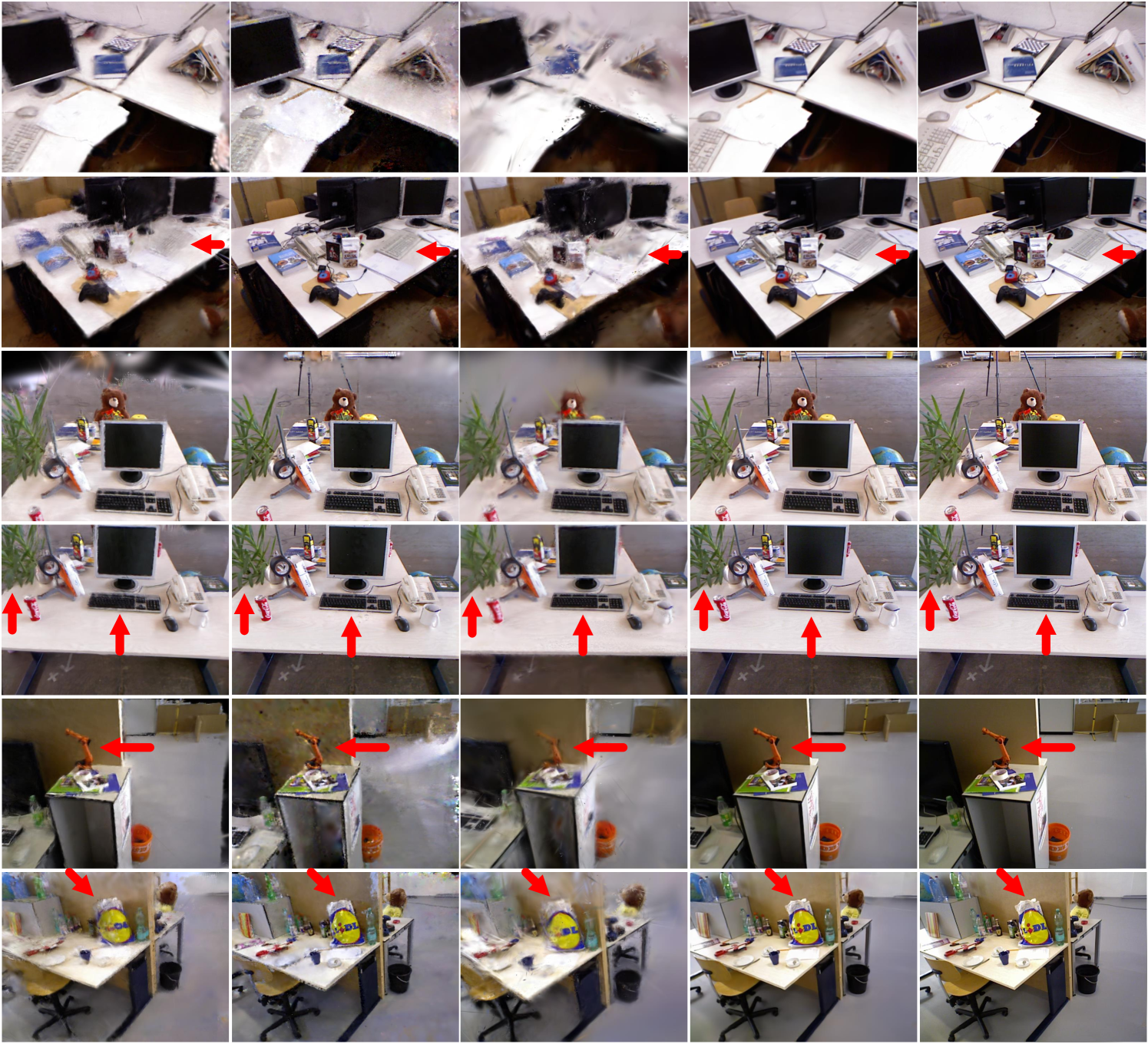
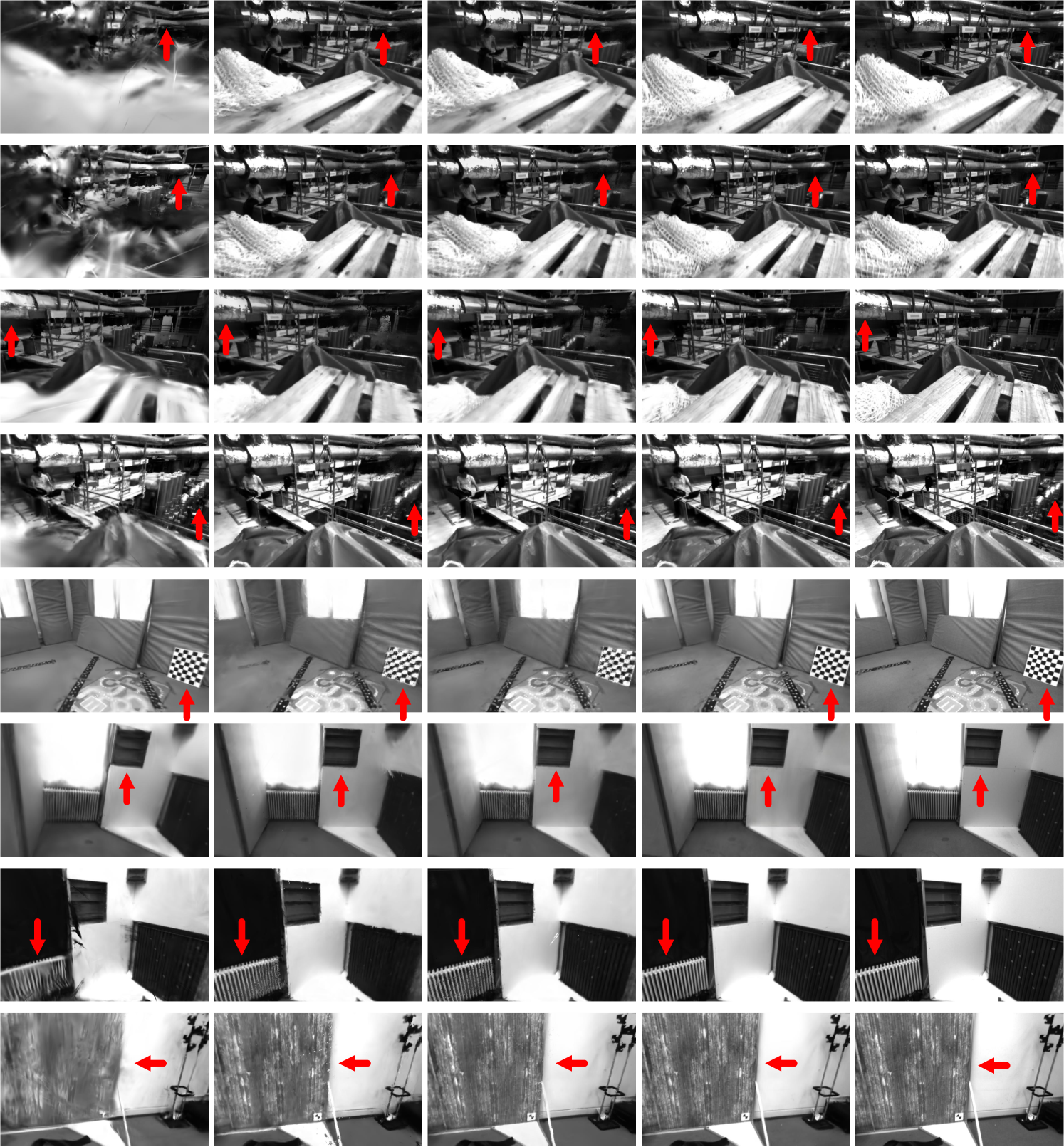
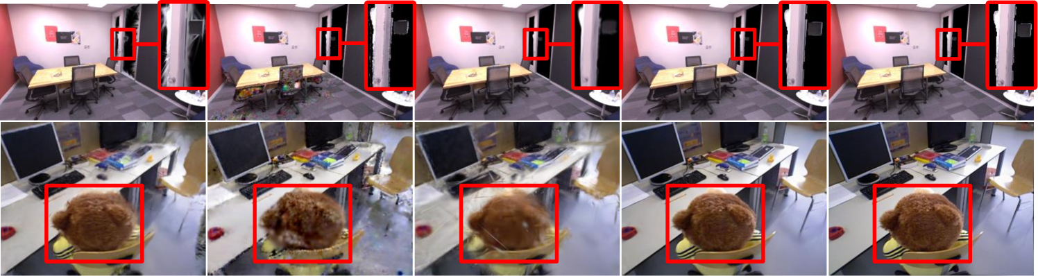
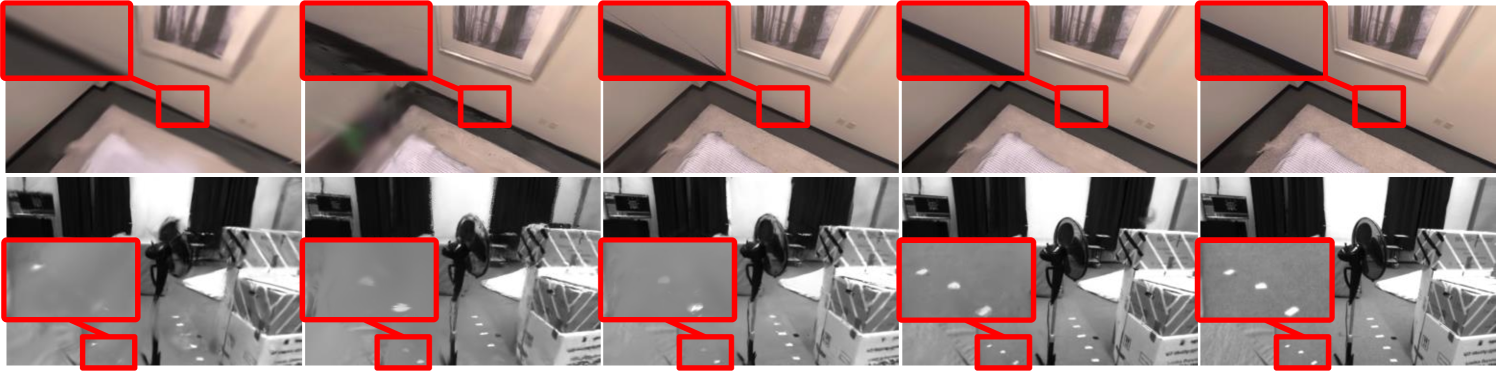
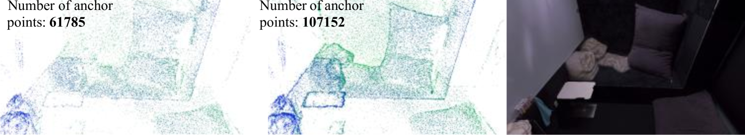
However, most SLAM algorithms based on 3D-GS have neglected the latent structure in the scene, which constrains their rendering quality. While some methods [14, 40, 27, 9, 11, 24, 43, 17, 39] have explored improvements in accuracy, efficiency, and semantics, insufficient structural exploitation remains a critical issue. For instance, as evidenced by the 2nd row in Fig. 1, MonoGS [24] produces a highly disorganized reconstruction of the ladder structure due to this limitation. In contrast, few methods, like Photo-SLAM [12], leverage scene structure. Photo-SLAM [12] initializes 3D Gaussians with point cloud obtained from indirect visual SLAM and incorporates a geometry-based densification module. In the original 3D-GS, 3D Gaussians are initialized from COLMAP [30] points. Since indirect visual SLAM and COLMAP [30] share similar pipeline structures, the generated point clouds exhibit similar intrinsic properties. Hence, the 3D Gaussians of Photo-SLAM [12] converge to a relatively optimal result with fewer iterations, yet it still underutilizes the underlying scene structure. The blurry reconstruction of the mouse edge by Photo-SLAM [12] is still apparent as shown in the 2nd row of Fig. 1.

Another partially unresolved challenge in these methods [14, 40, 27, 9, 11, 24, 12, 43, 17, 39] is the significant appearance variations within the scene (e.g., exposure, lighting). To address this issue, NeRF-W [23] refines the appearance embeddings (AE) in NRW [25] and introduces them into NeRF. However, AE has a notable limitation: its training involves each ground-truth image from the test set. In novel view synthesis tasks, the test set contains 12.5% of all views, whereas in SLAM tasks, this increases to 80%, making it more challenging for AE to accurately predict appearance in novel views. Additionally, these approaches [14, 40, 27, 9, 11, 24, 12, 21, 43, 17, 39] fail to capture high-frequency details (e.g., object edges, complex texture regions). FreGS [45] combines frequency regularization to model the local details, but its effectiveness is constrained by the use of a single-scale frequency spectrum.

To address the above limitations, this paper presents SEGS-SLAM, a novel 3D Gaussian Splatting SLAM system. First, we investigate the benefits of leveraging scene structure for improving rendering accuracy. While point cloud produced by ORB-SLAM3 [3] preserves strong latent structure, we observe that the anchor-based 3D Gaussians in [21] effectively leverage the underlying structure. Motivated by this, we propose a structure-enhanced photorealistic mapping (SEPM) framework, which initializes anchor points using ORB-SLAM3 [3] point cloud, significantly enhancing the utilization of scene structure. Experimental results validate the effectiveness of this simple yet powerful strategy, and we hope this insight will inspire further research in this direction. Second, we propose Appearance-from-Motion embedding (AfME), which takes poses as input and eliminates the need for training on the left half of each ground-truth image in the test set. We further introduce a frequency pyramid regularization (FPR) technique to better capture high-frequency details in the scene. The main contributions of this work are as follows:

1.

To our knowledge, structure-enhanced photorealistic mapping (SEPM) is the first SLAM framework that intializes anchor points with ORB-SLAM3 point cloud to strengthen the utilization of scene structure, leading to significant rendering improvements.
2.

We propose Appearance-from-Motion embedding (AfME), which models per-image appearance variations into a latent space extracted from camera pose.
3.

Extensive evaluations on various public datasets demonstrate that our method significantly surpasses state-of-the-art (SOTA) methods in photorealistic mapping quality across monocular, stereo, and RGB-D cameras, while maintaining competitive tracking accuracy.

2 Related Work

Visual SLAM. Traditional visual SLAM methods can be classified into two categories: indirect methods and direct methods. Indirect methods [16, 3] rely on extracting and tracking features between consecutive frames to estimate poses and build sparse maps by minimizing a reprojection error, including ORB-SLAM3 [3]. Direct methods [6, 7] estimate motion and structure by minimizing a photometric error, which can build sparse or semi-dense maps. Recently, some methods [1, 33, 35, 36, 18] have integrated deep learning into visual SLAM systems. Among them, the current SOTA method is Droid-SLAM [35]. More recently, Lipson et al. [18] combine optical flow prediction with a pose-solving layer to achieve camera tracking. Our approach favors traditional indirect visual SLAM.

Implicit Representation based SLAM. iMAP [34] pioneers the use of neural implicit representations to achieve tracking and mapping through reconstruction error. Subsequently, many works [50, 41, 4, 13, 37, 49, 22, 42, 51] have explored new representation forms, including voxel-based neural implicit surface representation [41], multi-scale tri-planes [13] and point-based neural implicit representation [28]. Recently, SNI-SLAM [49] and IBD-SLAM [42] introduce a hierarchical semantic representation and an xyz-map representation, respectively. Some works [48, 19, 5, 10, 29, 47, 44] address other challenges, including loop closure [48, 19]. However, most efforts focus on scene geometry reconstruction, with Point-SLAM [28] extending to novel view synthesis. Moreover, the NeRF models used in these methods do not account for appearance variations.

3D Gaussian Splatting based SLAM. Recently, an explicit representation, 3D-GS [15], is introduced into visual SLAM. Most methods enhance RGB-D SLAM in rendering quality [9, 14, 40, 43], efficiency [27, 9], robustness [11, 39], and semantics [17]. For example, GS-ICP SLAM[9] achieves photorealistic mapping by fusing 3D-GS with Generalized ICP. Few methods improve SLAM rendering accuracy and efficiency across monocular, stereo, and RGB-D cameras, with MonoGS [24] and Photo-SLAM [12] as exceptions. However, neither of these methods effectively leverages latent scene structures or enhances the modeling of scene details, which limits their rendering quality. To address this, our proposed SEGS-SLAM further reinforces the utilization of global scene structure.

Refer to caption — Figure 2: Overview of our method. Our method supports monocular, stereo, and RGB-D cameras. The input image stream is processed by the localization and geometric mapping modules, generating point cloud and accurate poses. SEPM incrementally initializes anchor points (middle) based on the point cloud (top left), which preserves the underlying structure. The poses are then fed into the AfME to model appearance variations in the scene. Additionally, we introduce FPR to improve the reconstruction of high-frequency details in the scene.

3 Preliminaries

In this section, we first introduce the structured 3D Gaussian splatting in [21]. Subsequently, we review the localization and mapping process of ORB-SLAM3 [3].

3.1 Structured 3D Gaussian Splatting

Structured 3D Gaussians is a hierarchical representation in [21]. They construct anchor points by voxelizing the point cloud obtained from COLMAP [30]. An anchor point is the center $\mathrm{\mathbf{t}}_{v}$ of a voxel, equipped with a context feature $\hat{f}_{v}\in\mathbb{R}^{32}$ , a scale factor $l_{v}\in\mathbb{R}^{3}$ , and a set of $k$ learnable offsets $\mathrm{\mathbf{O}}_{v}=\{\mathcal{O}_{0},\ldots,\mathcal{O}_{k-1}\}\in\mathbb{R}^{k\times 3}$ . For each anchor point $\mathrm{\mathbf{t}}_{v}$ , they generate $k$ 3D Gaussians, whose positions are calculated as:

\{\mu_{0},\ldots,\mu_{k-1}\}=\mathrm{\mathbf{t}}_{v}+\{\mathcal{O}_{0},\ldots,\mathcal{O}_{k-1}\}\cdot l_{v}.

(1)

Other parameters of $k$ 3D Gaussians are decoded using individual MLPs, denoted as $M_{\alpha}$ , $M_{c}$ , $M_{q}$ , and $M_{s}$ , respectively. The colors of the Gaussians are obtained as follows:

\{c_{0},\dots,c_{k-1}\}=M_{C}(\hat{f}_{v},\ \delta_{vc},\ \vec{\mathrm{\mathbf{d}}}_{vc}),

(2)

where $\delta_{vc}=\|\mathrm{\mathbf{t}}_{v}-\mathrm{\mathbf{t}}_{c}\|_{2}$ is the relative distance between camera position $\mathrm{\mathbf{t}}_{c}$ and an anchor point and $\vec{\mathrm{\mathbf{d}}}_{vc}=(\mathrm{\mathbf{t}}_{v}-\mathrm{\mathbf{t}}_{c})/\delta_{vc}$ is their viewing direction. The opacity $\{\alpha_{i}\}$ , quaternion $\{q_{i}\}$ , and scale $\{s_{i}\}$ are similarly obtained. After obtaining the parameters of each 3D Gaussian $G(x)$ within the view frustum, it is projected onto the image plane to form a 2D Gaussian $G^{\prime}_{i}(x^{\prime})$ . Following 3D-GS [15], a tile-based rasterizer is used to sort the 2D Gaussians, and $\alpha-$ blending is employed to complete the rendering:

C(x^{\prime})=\sum_{i\in N}c_{i}\delta_{i}\prod_{j=1}^{i-1}(1-\delta_{j}),\quad\delta_{i}=\alpha_{i}G^{\prime}_{i}(x^{\prime}),

(3)

where $x^{\prime}$ is the pixel position and $N$ is the number of corresponding 2D Gaussians for each pixel.

3.2 Localization and Geometry Mapping

ORB-SLAM3 [3] can track camera poses and generate point cloud accurately. The camera pose is represented as $(\mathrm{\mathbf{R}},\mathrm{\mathbf{t}})$ , where $\mathrm{\mathbf{R}}\in\mathrm{SO(3)}$ denotes orientation and $\mathrm{\mathbf{t}}\in\mathbb{R}^{3}$ represents position. The camera poses $(\mathrm{\mathbf{R}},\mathrm{\mathbf{t}})$ and the point cloud $\{\mathrm{\mathbf{P}}_{0},\dots,\mathrm{\mathbf{P}}_{\eta}\}\in\mathbb{R}^{\eta\times 3}$ of the scene can be solved through local or global bundle adjustment (BA):

	$\displaystyle\{\mathrm{\mathbf{P}}_{m},\mathrm{\mathbf{R}}_{l},\mathrm{\mathbf{t}}_{l}\}$	$\displaystyle=\mathop{\mathrm{argmin}}\limits_{\mathrm{\mathbf{P}}_{m},\mathrm{\mathbf{R}}_{l},\mathrm{\mathbf{t}}_{l}}\sum_{\kappa\in\mathcal{K}_{L}\cup\mathcal{K}_{F}}\sum_{j\in\mathcal{X}_{k}}\rho(E(\kappa,j)),$		(4)
	$\displaystyle E(\kappa,j)$	$\displaystyle=\\|\mathrm{\mathbf{p}}_{j}-\pi(\mathrm{\mathbf{R}}_{\kappa}\mathrm{\mathbf{P}}_{j}+\mathrm{\mathbf{t}}_{\kappa})\\|^{2}_{\Sigma_{g}},$		(5)

where $m\in{P}_{L}$ , $l\in\mathcal{K}_{L}$ , $\mathcal{K}_{L}$ is a set of covisible keyframes, ${P}_{L}$ are the points seen in $\mathcal{K}_{L}$ , $\mathcal{K}_{F}$ are other keyframes, $\mathcal{X}_{k}$ is the set of matched points between a keyframe $\kappa$ and ${P}_{L}$ , $\rho$ is the robust Huber cost function, $E(\kappa,j)$ is the reprojection error between the matched 3D points $\mathrm{\mathbf{P}}_{j}$ and 2D feature points $\mathrm{\mathbf{p}}_{j}$ , $\pi$ is the projection function, and $\Sigma_{g}$ denotes the covariance matrix associated with the keypoint’s scale. We provide more details in Sec. 11.2 of supplementary material.

4 SEGS-SLAM

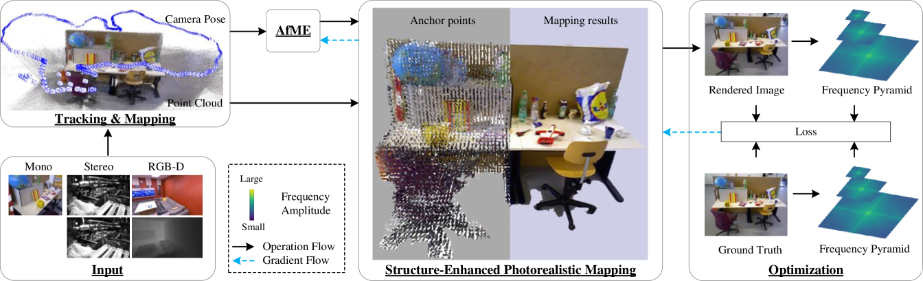
In this section, we first give an overview of our system. We then present details of two key innovations: SEPM and AfME. Finally, we provide an introduction to our training loss and FPR. The overview of our SEGS-SLAM is summarized in Fig. 2. First, the input image stream is processed through tracking and geometric mapping process in Sec. 3.2 to obtain camera poses and point cloud. On one hand, SEPM voxelizes the point cloud to initialize anchors, enhancing the exploitation of underlying scene structure. On the other hand, AfME encodes the camera poses to model appearance variations. Finally, the rendered images are supervised by ground-truth images, with the assistance of FPR, while jointly optimizing the parameters of the 3D Gaussians and the weights of AfME throughout training.

4.1 Structure-Enhanced Photorealistic Mapping

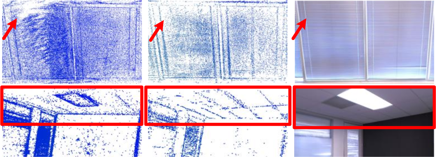
A common limitation of existing 3DGS-based SLAM systems is the gradual degradation of the underlying structure of Gaussians during optimization, limiting the quality of the rendered results. Our key insight is that preserving strong scene structure throughout the optimization process is crucial for achieving high-fidelity rendering. Inspired by this, we make several observations. First, ORB-SLAM3 [3] generates a point cloud that preserves the scene structure well. Photo-SLAM [12] initializes 3D Gaussians with the point cloud, but as shown in the Fig. 3 (a), relying solely on the latent structure of the point cloud is insufficient, as Gaussians still undergo structural degradation during optimization. We further observe that the hierarchical structure in [21] leverages scene structure, using anchor points to manage 3D Gaussians. These anchor points remain fixed during the optimization process, ensuring that 3D Gaussians retain the underlying structure of the scene.

Based on this observation, we propose incrementally voxelizing the point cloud $P_{k}$ of each keyframe to construct anchor points, as follows:

V_{k}=\{\lfloor\frac{P_{k}}{\epsilon}\rceil\}\cdot\epsilon,

(6)

where $V_{k}\in R^{N\times 3}$ denotes voxel centers, $\epsilon$ is the voxel size, and $\{\cdot\}$ is the operation to remove redundant points.

Fig. 2 visualizes this process. The ORB-SLAM3 point cloud (top left) is voxelized into the anchor points (middle), which preserve the underlying structure effectively. In this way, the structural prior from ORB-SLAM3’s point cloud and the anchor-based organization are seamlessly fused, enhancing the exploitation of the underlying structure. Specifically, the anchor points inherit the strong structural properties of the point cloud and, due to their fixed positions, consistently preserve the latent scene structure throughout training. As shown in the Fig. 3 (b), this effectively prevents structural degradation of Gaussians over training, a key issue in prior methods. This strategy yields substantial improvements in rendering accuracy, as demonstrated in our ablation studies. Although conceptually simple, our approach proves highly effective. After anchor points construction, 3D Gaussians are then generated according to Eq. 1, Eq. 8, and rendered via Eq. 3.

4.2 Appearance-from-Motion Embedding

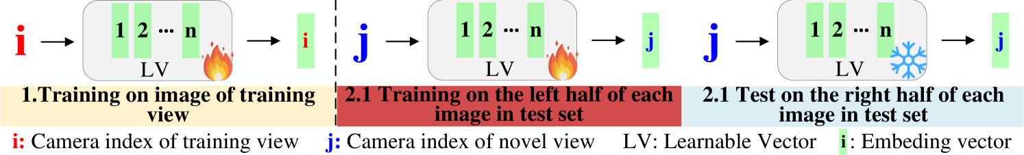
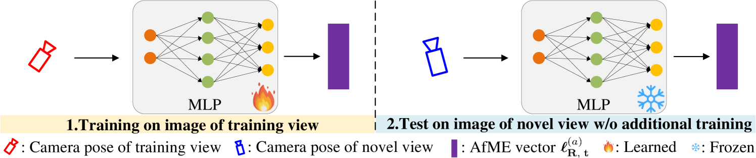
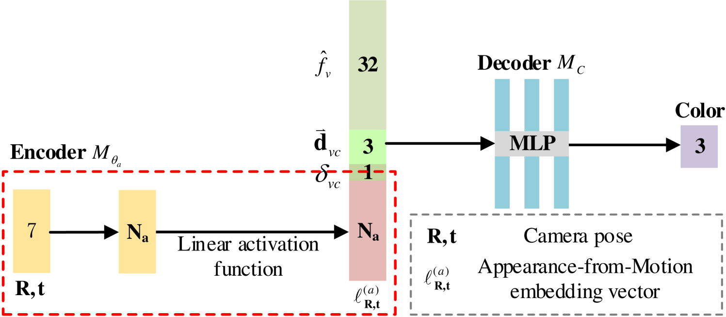
To further enhance the rendering quality of SEGS-SLAM, we observe a drop in the photorealistic mapping quality when suffering from appearance changes. AE is a proven solution in [23, 21] for handling such variations. However, the limitation of the AE in [23] lies in involving each ground-truth (left half of the image) in the test set for training as shown in the mid of Fig. 4 (a). To address this issue, we propose Appearance-from-Motion embedding (AfME), which employs a lightweight Multilayer Perceptron (MLP) $M_{\theta_{a}}$ to learn a shared appearance representation. As illustrated in Fig. 4 (b), the input of the encoder $M_{\theta_{a}}$ is the the camera pose $(\mathrm{\mathbf{R}},\ \mathrm{\mathbf{t}})$ . The MLP encodes the pose and outputs an embedding vector $\bm{\ell}^{(a)}_{\mathrm{\mathbf{R}},\ \mathrm{\mathbf{t}}}$ , as shown below:

\bm{\ell}^{(a)}_{\mathrm{\mathbf{R}},\ \mathrm{\mathbf{t}}}=M_{\theta_{a}}(\mathrm{\mathbf{R}},\ \mathrm{\mathbf{t}}).

(7)

Subsequently, the embedding vector $\bm{\ell}^{(a)}_{\mathrm{\mathbf{R}},\ \mathrm{\mathbf{t}}}$ is fed into the color decoder $M_{C}$ . After introducing AfME, the color prediction of 3D Gaussians changes from Eq. 2 to:

\{c_{0},\dots,c_{k-1}\}=M_{C}(\hat{f}_{v},\ \delta_{vc},\ \vec{\mathrm{\mathbf{d}}}_{vc},\ \bm{\ell}^{(a)}_{\mathrm{\mathbf{R}},\ \mathrm{\mathbf{t}}}).

(8)

More details are in Sec. 11.4 of supplementary material. We choose camera poses as inputs for several reasons: 1) Similar to image indices, camera poses are unique for each view. 2) Camera poses naturally represent spatial information, enabling AfME to predict appearance from spatial context. 3) Camera poses are more continuous than image indices.

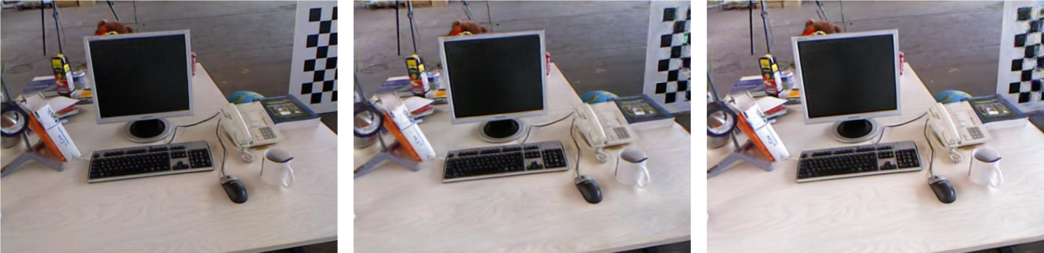
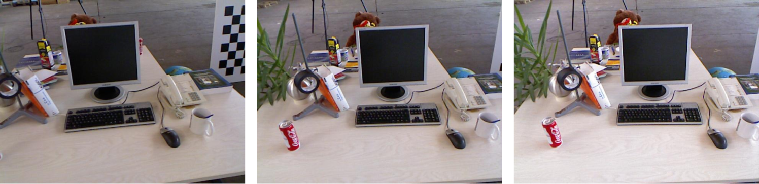
We adopt AfME to encode the scene appearance into the continuous pose space. Through training on the training set, AfME learns the mapping between appearance and camera pose, enabling it to predict the appearance for novel views. We conduct an experiment to demonstrate this. After training, we fix $\hat{f}_{v},\ \delta_{vc},\ \vec{\mathrm{\mathbf{d}}}_{vc}$ in the input of Eq. 8 and vary only the pose $\{\mathrm{\mathbf{R}},\ \mathrm{\mathbf{t}}\}$ fed into AfME. As shown in Fig. 5, the lighting conditions under the same view change consistently with the pose $\{\mathrm{\mathbf{R}},\ \mathrm{\mathbf{t}}\}$ , matching the illumination of corresponding viewpoints. This demonstrates that the illumination conditions can be embedded by AfME effectively.

4.3 Frequency Pyramid Regularization

A minor improvement is the frequency pyramid regularization (FPR), which leverages multi-scale frequency representation to enhance the reconstruction of high-frequency details in the scene. To achieve this, we apply bilinear interpolation to downsample both the render images $I_{r}$ and the ground truth images $I_{g}$ . Let $s\in\mathcal{S}=\{s_{0},s_{1},\ldots,s_{n}\}$ denote the scale of an image. We apply a 2D Fast Fourier Transform (FFT) to obtain the frequency spectra $\mathcal{F}(I_{r}^{s})(u,v),\mathcal{F}(I_{g}^{s})(u,v)$ . The loss $\mathcal{L}_{hf}$ is computed as

	$\displaystyle\mathcal{L}_{hf}=\sum_{s\in\mathcal{S}}\frac{1}{\mathcal{N}}\lambda_{s}\sum_{u,v}\left\|F_{hf,r}^{s}(u,v)-F_{hf,g}^{s}(u,v)\right\|,$		(9)
	$\displaystyle F_{hf,i}^{s}(u,v)=H_{hf}(u,v)\cdot\mathcal{F}(I_{i}^{s})(u,v),\ i\in\{r,g\},$		(10)

where $F_{hf,r}^{s}(u,v),F_{hf,g}^{s}(u,v)$ is the high-frequency extracted by a high-pass filter $H_{hf}(u,v)$ , $\mathcal{N}=HW$ denotes the image size, and $\lambda_{s}$ represents the weight of each scale. More details are in Sec. 8 of supplementary material.

4.4 Losses Design

The optimization of the learnable parameters, the MLP $M_{\alpha}$ , $M_{c}$ , $M_{q}$ , $M_{s}$ , and $M_{\theta_{a}}$ , are achieved by minimizing the L1 loss $\mathcal{L}_{1}$ , SSIM term [38] $\mathcal{L}_{\text{SSIM}}$ , frequency regularization $\mathcal{L}_{hf}$ , and volume regularization [20] $\mathcal{L}_{\text{vol}}$ between the rendered images and the ground truth images, denoted as

\mathcal{L}=(1-\lambda)\mathcal{L}_{1}+\lambda(1-\mathcal{L}_{\text{SSIM}})+\lambda_{\text{vol}}\mathcal{L}_{\text{vol}}+\lambda_{hf}\mathcal{L}_{hf}.

(11)

Following [21], we also incorporate $\mathcal{L}_{\text{vol}}$ .

Datasets (Camera)	Replica (RGB-D)			TUM RGB-D (RGB-D)
Method	PSNR $\uparrow$	SSIM $\uparrow$	LPIPS $\downarrow$	PSNR $\uparrow$	SSIM $\uparrow$	LPIPS $\downarrow$
MonoGS [24]	36.81	0.964	0.069	24.11	0.800	0.231
Photo-SLAM [12]	35.50	0.949	0.056	20.99	0.736	0.213
Photo-SLAM-30K	36.94	0.952	0.040	21.73	0.757	0.186
RTG-SLAM [27]	32.79	0.918	0.124	16.47	0.574	0.461
GS-SLAM^∗ [40]	34.27	0.975	0.082	-	-	-
SplaTAM [14]	33.85	0.936	0.099	21.41	0.764	0.265
SGS-SLAM [17]	33.96	0.969	0.099	-	-	-
GS-ICP SLAM [9]	37.14	0.968	0.045	17.81	0.642	0.361
Ours	39.42	0.975	0.021	26.03	0.843	0.107

Table 1: Quantitative evaluation of our method compared to SOTA methods for RGB-D camera on Replica and TUM RGB-D datasets. Best results are marked as best score, second best score and third best score. GS-SLAM^∗ denotes the result of GS-SLAM is taken from [40], all others are obtained in our experiments. ’-’ denotes the system does not provide valid results.

Datasets (Camera)	Replica (Mono)			TUM RGB-D (Mono)			EuRoC (Stereo)
method	PSNR $\uparrow$	SSIM $\uparrow$	LPIPS $\downarrow$	PSNR $\uparrow$	SSIM $\uparrow$	LPIPS $\downarrow$	PSNR $\uparrow$	SSIM $\uparrow$	LPIPS $\downarrow$
MonoGS [24]	28.34	0.878	0.256	21.00	0.705	0.393	22.60	0.789	0.274
Photo-SLAM [12]	33.60	0.934	0.077	20.17	0.708	0.224	11.90	0.409	0.439
Photo-SLAM-30K	36.08	0.947	0.054	21.06	0.733	0.186	11.77	0.405	0.430
Ours	37.96	0.964	0.037	25.17	0.825	0.122	23.64	0.791	0.182

Table 2: Quantitative evaluation of our method compared to SOTA methods for Monocular (Mono) and Stereo cameras on Replica, TUM RGB-D, and EuRoC MAV datasets. Best results are marked as best score and second best score.

5 Experiment

5.1 Experiment Setup

Implementation. Our SEGS-SLAM is fully implemented using the LibTorch framework with C++ and CUDA. The training and rendering of 3D Gaussians involves three key modules: SEPM, AfME, and FPR, operating as a parallel thread alongside the localization and geometric mapping process. SEGS-SLAM trains the 3D Gaussians using only keyframe images, point clouds, and poses, where keyframes are selected based on co-visibility. In each iteration, SEGS-SLAM randomly samples a viewpoint from the current set of keyframes. We use the images and poses of keyframes as the training set, while the remaining images and poses serve as the test set. Moreover, following FreGS [45], we activate FPR once the structure of anchor points stabilizes and terminate it based on the completion of anchor point densification. The scale level of FPR is set to 3. Except for the non-open-source GS-SLAM [40], all methods compared in this paper are run on the same machine using their official code. The machine is equipped with an NVIDIA RTX 4090 GPU and a Ryzen 5995WX CPU. By default, our method runs for 30K iterations. The voxel size $\epsilon$ is $0.001\,\text{m}$ . For Eq. 11, we set $\lambda=0.2,\lambda_{\text{vol}}=0.01,\lambda_{hf}=0.01$ .

Baselines. We first list the baseline methods used to evaluate photorealistic mapping. For monocular and stereo cameras, we compare our method with Photo-SLAM [12], MonoGS [24], and Photo-SLAM-30K. For RGB-D cameras, we additionally include comparisons with RTG-SLAM [27], GS-SLAM [40], SplaTAM [14], SGS-SLAM [17], and GS-ICP SLAM [9], all of which represent SOTA SLAM methods based on 3D-GS. To ensure fairness, we set the maximum iteration limit to 30K for all methods, following the original 3D-GS [15]. Photo-SLAM-30K refers to Photo-SLAM [12] with a fixed iteration count of 30K. For camera pose estimation, we also compare ours with ORB-SLAM3 [3] and DROID-SLAM [35].

Metrics. We follow the evaluation protocol of MonoGS [24] to assess both camera pose estimation and novel view synthesis. For camera pose estimation, we report the root mean square error (RMSE) of the absolute trajectory error (ATE) [8] for all frames. For photorealistic mapping, we report standard rendering quality metrics, including PSNR, SSIM, and LPIPS [46]. To evaluate the photorealistic mapping quality, we only calculate the average metrics over novel views for all methods. We report the average across five runs for all methods. To ensure fairness, no training views are included in the evaluation, and for all RGB-D SLAM methods, no masks are applied to either the rendered or ground truth images during metric calculation. As a result, the reported metrics for Photo-SLAM [12] are slightly lower than those in the original paper, as they averages both novel and training views. Similarly, the metrics of SplaTAM [14], SGS-SLAM [17], and GS-ICP SLAM [9] are slightly lower than reported, as the original methods use a mask to exclude outliers for both the rendered and ground truth images based on anomalies in the depth image.

Datasets. Following [12, 40, 9, 14, 24, 11, 27, 28, 34, 17], we evaluate all methods on all sequences of the Replica dataset [31] for monocular and RGB-D cameras. Following [12, 40, 9, 24, 27, 34, 50], we use the fr1/desk, fr2/xyz, and fr3/office sequences of the TUM RGB-D dataset [32] for monocular and RGB-D cameras. Following [12], we use the MH01, MH02, V101, and V201 sequences of the EuRoC MAV dataset [2] for stereo cameras.

Camera Type	RGB-D			Monocular			Stereo
Datasets	Replica	TUM R	Avg.	Replica	TUM R	Avg.	EuRoC
Method	RMSE $\downarrow$	RMSE $\downarrow$	RMSE $\downarrow$	RMSE $\downarrow$	RMSE $\downarrow$	RMSE $\downarrow$	RMSE $\downarrow$
ORB-SLAM3 [3]	1.780	2.196	1.988	51.744	46.004	48.874	10.907
DRIOD-SLAM [35]	74.264	74.216	74.24	76.600	1.689	39.145	1.926
MonoGS [24]	0.565	1.502	1.033	37.054	4.009	63.437	49.241
Photo-SLAM [12]	0.582	1.870	1.226	0.930	1.539	1.235	11.023
RTG-SLAM [27]	0.191	0.985	0.581	-	-	-	-
GS-SLAM^∗ [40]	0.500	3.700	2.100	-	-	-	-
SplaTAM [14]	0.343	4.215	2.279	-	-	-	-
SGS-SLAM [17]	0.365	-	-	-	-	-	-
GS-ICP SLAM [9]	0.177	2.921	1.549	-	-	-	-
Ours	0.430	1.528	0.979	0.833	1.505	1.169	7.462

Table 3: Camera tracking result on Replica, TUM RGB-D (TUM R), and EuRoC MAV datasets for Monocular, stereo, and RGB-D cameras. RMSE of ATE (cm) is reported. The best results are marked as best score, second best score and third best score. ’-’ denotes that the system does not provide valid results.

5.2 Results Analysis

Camera Tracking Accuracy. As shown in Tab. 3, our method demonstrates competitive accuracy in tracking for monocular, stereo, and RGB-D cameras when compared with SOTA methods. This highlights the advantage of indirect visual SLAM in terms of localization accuracy.

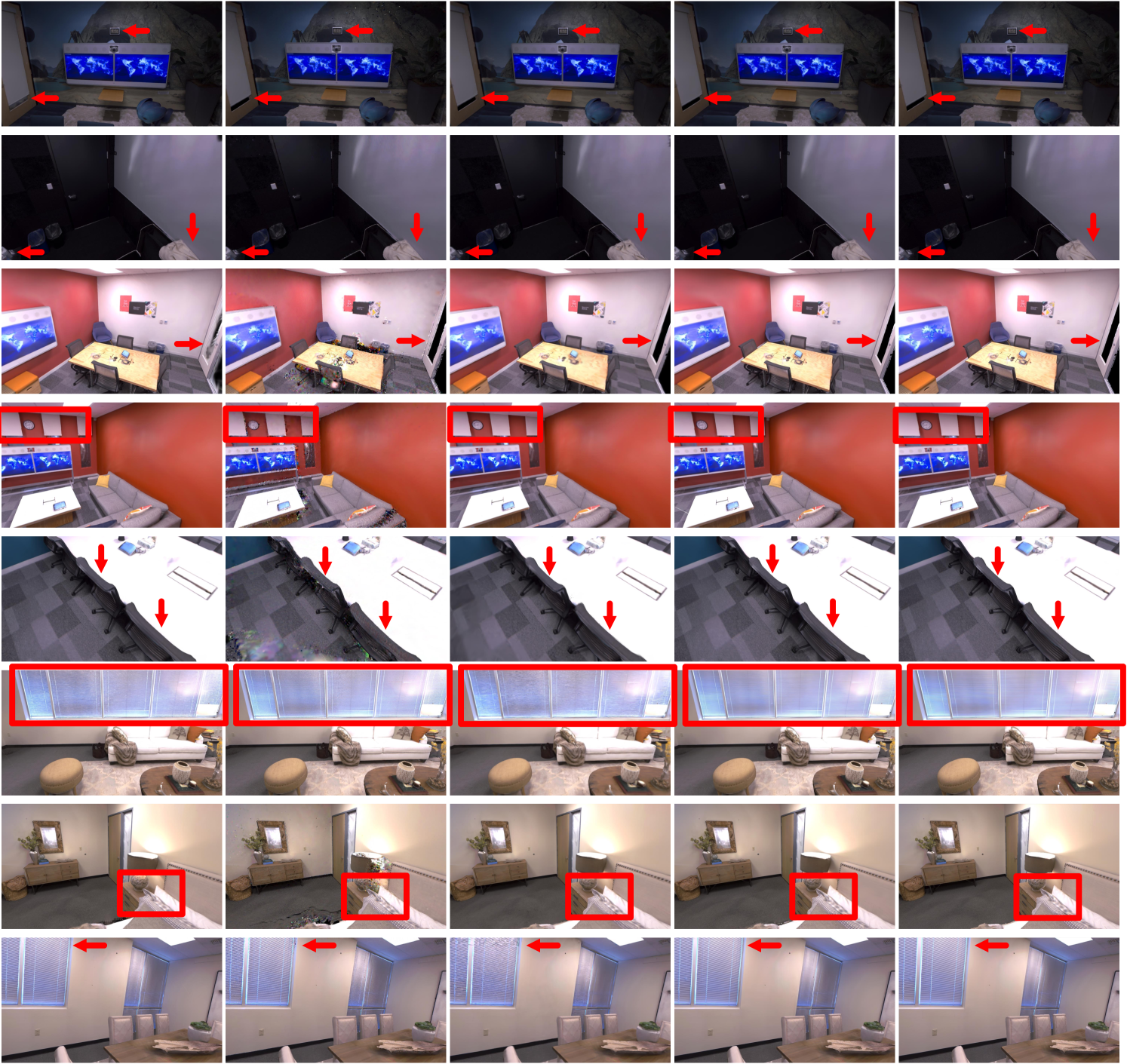
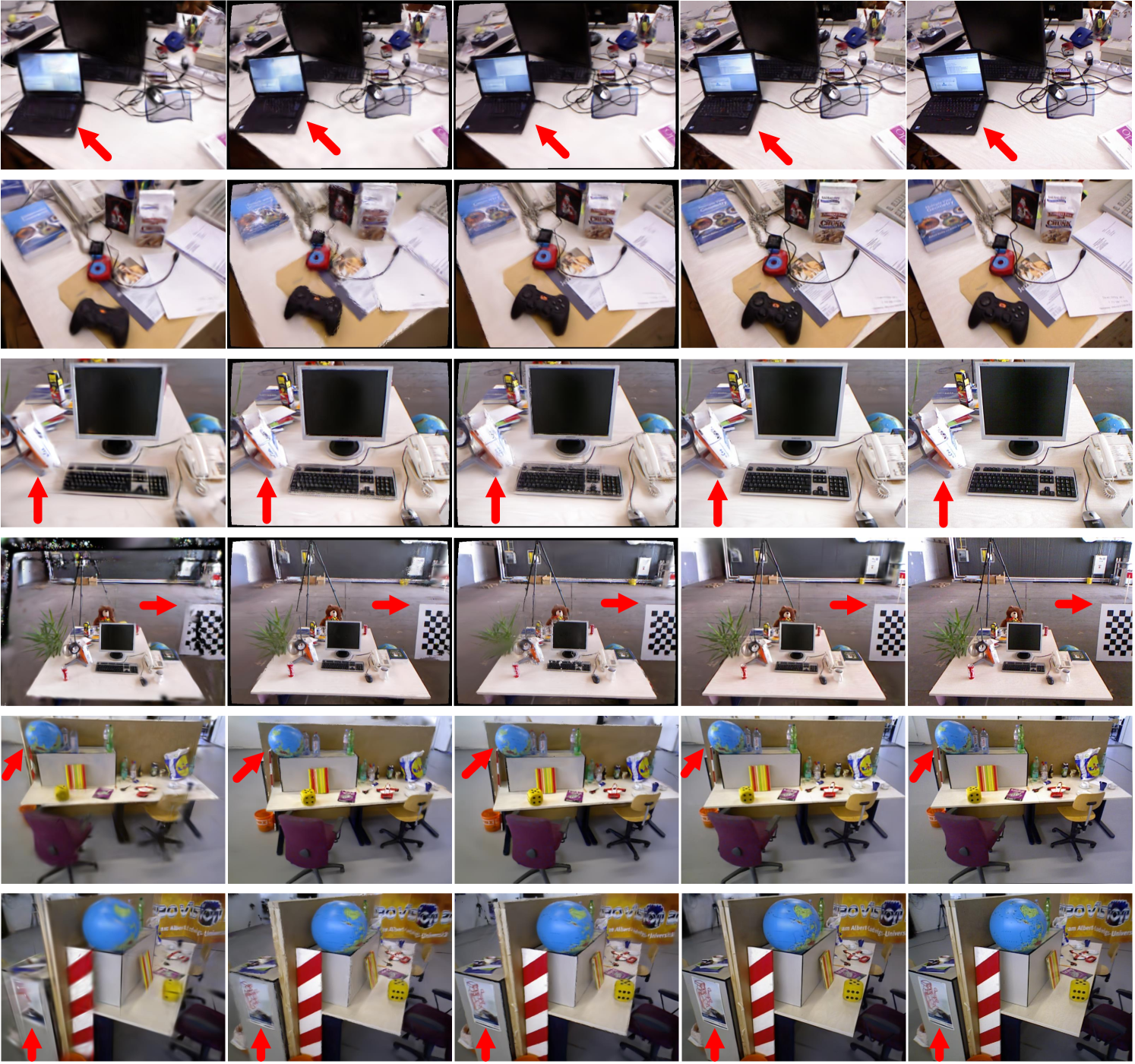
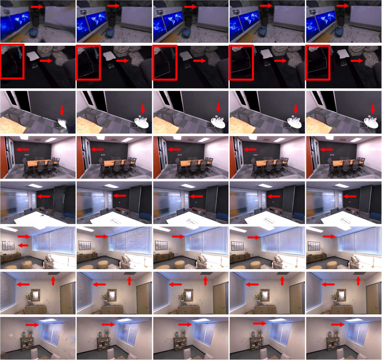
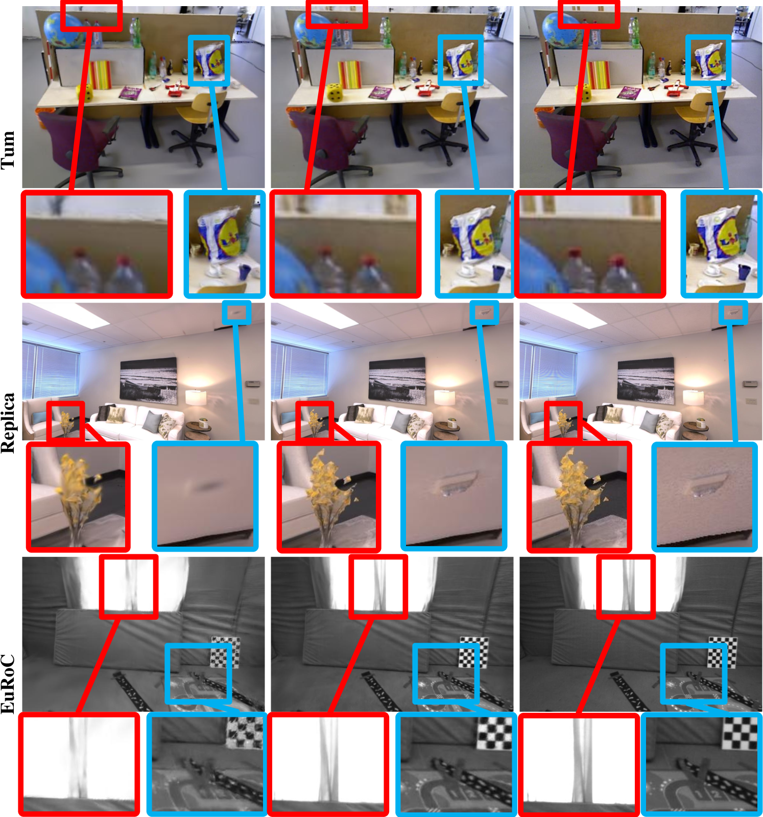
Novel View synthesis. The quantitative rendering results for novel views in RGB-D scenarios are shown in Tab. 1, where SEGS-SLAM significantly outperforms comparison methods, achieving the highest average rendering quality on both TUM RGB-D and Replica datasets. In the top of Fig. 6, it is evident that for the Replica dataset, only our method can accurately recover the contours of edge regions. The TUM RGB-D dataset presents a greater challenge compared with the Replica dataset, with highly cluttered scene structures and substantial lighting variations. GS-ICP SLAM [9], a leading RGB-D SLAM method based on 3D-GS, achieves the second-highest rendering accuracy on the Replica dataset. However, it relies heavily on depth images. As shown in the bottom of Fig. 6, GS-ICP SLAM [9] and other methods perform poorly on the TUM RGB-D dataset. Our SEGS-SLAM better reconstructs scene structure and lighting variations, benefiting from our SEPM and the AfME.

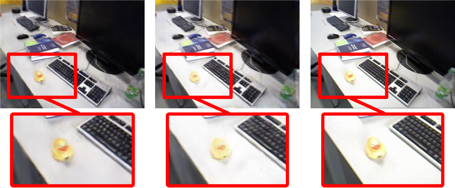
Tab. 2 presents quantitative rendering results for monocular scenarios, where SEGS-SLAM surpasses other methods. Notably, SEGS-SLAM continues to significantly outperform comparison methods on the TUM RGB-D dataset. Importantly, compared with RGB-D scenarios, MonoGS [24] experiences a sharp decline. The top of Fig. 7 further demonstrates that on the Replica dataset, our method effectively models high-frequency details more realistically in regions such as the edge of the wall.

Moreover, our method remains effective in stereo scenarios. The corresponding quantitative results for realistic mapping are recorded in Tab. 2, where our method achieves the highest rendering quality, surpassing the current SOTA method, MonoGS [24]. As shown in the bottom of Fig. 7, our approach better reconstructs the global structure and local details of the scene. We highlight that a key factor enabling our method to achieve superior performance across different camera types and datasets is the proposed SEPM. Its enhancement to rendering quality is highly generalizable, as further demonstrated in ablation studies.

5.3 Ablation Studies

Structure-Enhanced photorealistic mapping. To evaluate the impact of SEPM on photorealistic mapping metrics, we additionally train two variants of our method: one without SEPM, AfME, and FPR, and another without AfME and FPR. The variant without SEPM, AfME, and FPR directly uses the original 3D-GS [15]. As shown in Tab. 4, rows (1) and (2), introducing SEPM consistently yields significant improvements in rendering quality across all scenes. This validates the effectiveness of enhancing the exploitation of latent structure. Moreover, it demonstrates that SEPM has strong generalization across diverse camera inputs and datasets, inspiring future research. Notably, with only SEPM, our rendering metrics surpass existing SOTA methods. To further illustrate the benefits of SEPM, Fig. 8 presents visual comparisons, where a more complete and accurate scene structure leads to superior rendering quality.

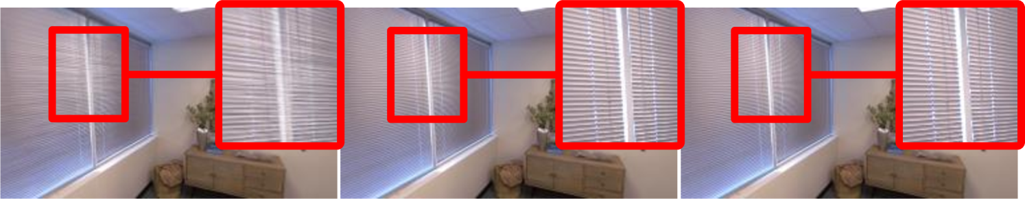
Appearance-from-Motion embedding. To evaluate the impact of the proposed AfME, we train an additional model for our method without AfME. In the rows (4) and (5) of Tab. 4, our full method (5) outperforms the model without AfME (4) in terms of PSNR scores. As shown in the top of Fig. 9, the AfME effectively predicts the lighting conditions of novel views. On the Replica dataset, the improvements from AfME are relatively modest. Replica is an easier dataset, in which PSNR already exceeds 37 without AfME, indicating that scene is well-reconstructed. Although incorporating AfME still yields a PSNR gain, the benefits are much more pronounced on the challenging TUM dataset, as clearly observed in both Fig. 9 and Tab. 4.

Frequency pyramid regularization. To evaluate the effect of the proposed FPR on photorealistic mapping metrics, we train an additional model for our method without FPR. As shown in Tab. 4, rows (3) and (5), our full method (5) surpasses the model without FPR (3) in terms of PSNR scores. Additionally, after applying the FPR, the model renders finer details in highly textured regions, as demonstrated by the curtain at the bottom of Fig. 9.

Camera type		RGB-D		Mono		Stereo
Datasets		Replica	TUM R	Replica	TUM R	EuRoC
#	Method	PSNR $\uparrow$	PSNR $\uparrow$	PSNR $\uparrow$	PSNR $\uparrow$	PSNR $\uparrow$
(1)	w/o FPR, AfME, SEPM	36.07	21.73	35.46	21.10	11.76
(2)	w/o FPR, AfME	38.98	24.20	36.31	23.54	22.91
(3)	w/o FPR	39.18	25.04	36.44	24.91	23.52
(4)	w/o AfME	39.12	24.66	37.48	23.69	22.99
(5)	Ours	39.42	26.03	37.96	25.17	23.64

Table 4: Ablation Study on the key components (1) - (5). The best results are marked as best score.

5.4 Limitations

One limitation of our method is that a poorly structured point cloud leads to a decline in photorealistic mapping quality. Additionally, while our method achieves real-time tracking and rendering at 17 and 400 FPS, respectively, it exhibits reduced rendering speed due to the increased number of 3D Gaussians used to model high-frequency details. Currently, AFME is only capable of handling static scenes. By encoding more complex inputs, it can tackle more sophisticated dynamic scenarios.

6 Conclusion

We propose a novel SLAM system with progressively refined 3D-GS, termed SEGS-SLAM. Experimental results show that our method surpasses SOTA methods in rendering quality across monocular, stereo, and RGB-D datasets. We demonstrate that by enhancing the utilization of the underlying scene structure, SEPM improves the visual quality of rendering. Furthermore, our proposed AfME and FPR effectively predict the appearance of novel views and refine the scene details, respectively.

Acknowledgements: This work is supported by the National Natural Science Foundation of China under Grant 62233011.

References

Bloesch et al. [2018] Michael Bloesch, Jan Czarnowski, Ronald Clark, Stefan Leutenegger, and Andrew J. Davison. Codeslam — learning a compact, optimisable representation for dense visual slam. In IEEE/CVF Conference on Computer Vision and Pattern Recognition, 2018.
Burri et al. [2016] Michael Burri, Janosch Nikolic, Pascal Gohl, Thomas Schneider, Joern Rehder, Sammy Omari, Markus W Achtelik, and Roland Siegwart. The euroc micro aerial vehicle datasets. The International Journal of Robotics Research, 35(10):1157–1163, 2016.
Campos et al. [2021] Carlos Campos, Richard Elvira, Juan J. Gómez Rodríguez, José M. M. Montiel, and Juan D. Tardós. Orb-slam3: An accurate open-source library for visual, visual–inertial, and multimap slam. IEEE Transactions on Robotics, 37(6):1874–1890, 2021.
Chung et al. [2023] Chi-Ming Chung, Yang-Che Tseng, Ya-Ching Hsu, Xiang-Qian Shi, et al. Orbeez-slam: A real-time monocular visual slam with orb features and nerf-realized mapping. In 2023 IEEE International Conference on Robotics and Automation, pages 9400–9406, 2023.
Deng et al. [2024] Tianchen Deng, Guole Shen, Tong Qin, Jianyu Wang, Wentao Zhao, Jingchuan Wang, Danwei Wang, and Weidong Chen. Plgslam: Progressive neural scene represenation with local to global bundle adjustment. In IEEE/CVF Conference on Computer Vision and Pattern Recognition, pages 19657–19666, 2024.
Engel et al. [2014] Jakob Engel, Thomas Schöps, and Daniel Cremers. Lsd-slam: Large-scale direct monocular slam. In European Conference on Computer Vision, pages 834–849, 2014.
Engel et al. [2018] Jakob Engel, Vladlen Koltun, and Daniel Cremers. Direct sparse odometry. IEEE Transactions on Pattern Analysis and Machine Intelligence, 40(3):611–625, 2018.
Grupp [2017] Michael Grupp. evo: Python package for the evaluation of odometry and slam. https://github.com/MichaelGrupp/evo, 2017.
Ha et al. [2024] Seongbo Ha, Jiung Yeon, and Hyeonwoo Yu. Rgbd gs-icp slam. In European Conference on Computer Vision, pages 180–197, 2024.
Hu et al. [2023] Jiarui Hu, Mao Mao, Hujun Bao, Guofeng Zhang, and Zhaopeng Cui. Cp-slam: Collaborative neural point-based slam system. In Advances in Neural Information Processing Systems, pages 39429–39442, 2023.
Hu et al. [2024] Jiarui Hu, Xianhao Chen, Boyin Feng, Guanglin Li, Liangjing Yang, Hujun Bao, Guofeng Zhang, and Zhaopeng Cui. Cg-slam: Efficient dense rgb-d slam in a consistent uncertainty-aware 3d gaussian field. In European Conference on Computer Vision, pages 93–112, 2024.
Huang et al. [2024] Huajian Huang, Longwei Li, Hui Cheng, and Sai-Kit Yeung. Photo-slam: Real-time simultaneous localization and photorealistic mapping for monocular stereo and rgb-d cameras. In IEEE/CVF Conference on Computer Vision and Pattern Recognition, pages 21584–21593, 2024.
Johari et al. [2023] Mohammad Mahdi Johari, Camilla Carta, and François Fleuret. Eslam: Efficient dense slam system based on hybrid representation of signed distance fields. In IEEE/CVF Conference on Computer Vision and Pattern Recognition, pages 17408–17419, 2023.
Keetha et al. [2024] Nikhil Keetha, Jay Karhade, Krishna Murthy Jatavallabhula, Gengshan Yang, Sebastian Scherer, Deva Ramanan, and Jonathon Luiten. Splatam: Splat track & map 3d gaussians for dense rgb-d slam. In IEEE/CVF Conference on Computer Vision and Pattern Recognition, pages 21357–21366, 2024.
Kerbl et al. [2023] Bernhard Kerbl, Georgios Kopanas, Thomas Leimkühler, and George Drettakis. 3D Gaussian Splatting for Real-Time Radiance Field Rendering. ACM Transactions on Graphics, 42(4):1–14, 2023.
Klein and Murray [2007] Georg Klein and David Murray. Parallel tracking and mapping for small ar workspaces. In 2007 6th IEEE and ACM International Symposium on Mixed and Augmented Reality, pages 225–234, 2007.
Li et al. [2025] Mingrui Li, Shuhong Liu, Heng Zhou, Guohao Zhu, Na Cheng, Tianchen Deng, and Hongyu Wang. Sgs-slam: Semantic gaussian splatting for neural dense slam. In European Conference on Computer Vision, pages 163–179, 2025.
Lipson and Deng [2024] Lahav Lipson and Jia Deng. Multi-session slam with differentiable wide-baseline pose optimization. In IEEE/CVF Conference on Computer Vision and Pattern Recognition, pages 19626–19635, 2024.
Liso et al. [2024] Lorenzo Liso, Erik Sandström, Vladimir Yugay, Luc Van Gool, and Martin R. Oswald. Loopy-slam: Dense neural slam with loop closures. In IEEE/CVF Conference on Computer Vision and Pattern Recognition, pages 20363–20373, 2024.
Lombardi et al. [2021] Stephen Lombardi, Tomas Simon, Gabriel Schwartz, Michael Zollhoefer, Yaser Sheikh, and Jason Saragih. Mixture of volumetric primitives for efficient neural rendering. ACM Transactions on Graphics, 40(4), 2021.
Lu et al. [2024] Tao Lu, Mulin Yu, Linning Xu, Yuanbo Xiangli, Limin Wang, Dahua Lin, and Bo Dai. Scaffold-gs: Structured 3d gaussians for view-adaptive rendering. In IEEE/CVF Conference on Computer Vision and Pattern Recognition, pages 20654–20664, 2024.
Mao et al. [2024] Yunxuan Mao, Xuan Yu, Zhuqing Zhang, Kai Wang, Yue Wang, Rong Xiong, and Yiyi Liao. Ngel-slam: Neural implicit representation-based global consistent low-latency slam system. In 2024 IEEE International Conference on Robotics and Automation, pages 6952–6958, 2024.
Martin-Brualla et al. [2021] Ricardo Martin-Brualla, Noha Radwan, Mehdi S. M. Sajjadi, Jonathan T. Barron, Alexey Dosovitskiy, and Daniel Duckworth. Nerf in the wild: Neural radiance fields for unconstrained photo collections. In IEEE/CVF Conference on Computer Vision and Pattern Recognition, pages 7210–7219, 2021.
Matsuki et al. [2024] Hidenobu Matsuki, Riku Murai, Paul H.J. Kelly, and Andrew J. Davison. Gaussian splatting slam. In IEEE/CVF Conference on Computer Vision and Pattern Recognition, pages 18039–18048, 2024.
Meshry et al. [2019] Moustafa Meshry, Dan B. Goldman, Sameh Khamis, Hugues Hoppe, Rohit Pandey, Noah Snavely, and Ricardo Martin-Brualla. Neural rerendering in the wild. In IEEE/CVF Conference on Computer Vision and Pattern Recognition, 2019.
Mildenhall et al. [2020] Ben Mildenhall, Pratul P. Srinivasan, Matthew Tancik, Jonathan T. Barron, Ravi Ramamoorthi, and Ren Ng. Nerf: Representing scenes as neural radiance fields for view synthesis. In European Conference on Computer Vision, pages 405–421, 2020.
Peng et al. [2024] Zhexi Peng, Tianjia Shao, Yong Liu, Jingke Zhou, Yin Yang, Jingdong Wang, and Kun Zhou. Rtg-slam: Real-time 3d reconstruction at scale using gaussian splatting. In ACM SIGGRAPH, 2024.
Sandström et al. [2023a] Erik Sandström, Yue Li, Luc Van Gool, and Martin R. Oswald. Point-slam: Dense neural point cloud-based slam. In IEEE/CVF International Conference on Computer Vision, pages 18433–18444, 2023a.
Sandström et al. [2023b] Erik Sandström, Kevin Ta, Luc Van Gool, and Martin R. Oswald. Uncle-slam: Uncertainty learning for dense neural slam. In IEEE/CVF International Conference on Computer Vision Workshops, pages 4537–4548, 2023b.
Schönberger and Frahm [2016] Johannes Lutz Schönberger and Jan-Michael Frahm. Structure-from-motion revisited. In Conference on Computer Vision and Pattern Recognition, 2016.
Straub et al. [2019] Julian Straub, Thomas Whelan, Lingni Ma, Yufan Chen, Erik Wijmans, Simon Green, Jakob J Engel, et al. The replica dataset: A digital replica of indoor spaces. arXiv preprint arXiv:1906.05797, 2019.
Sturm et al. [2012] Jürgen Sturm, Nikolas Engelhard, Felix Endres, Wolfram Burgard, and Daniel Cremers. A benchmark for the evaluation of rgb-d slam systems. In IEEE/RSJ International Conference on Intelligent Robots and Systems, pages 573–580, 2012.
Sucar et al. [2020] Edgar Sucar, Kentaro Wada, and Andrew Davison. Nodeslam: Neural object descriptors for multi-view shape reconstruction. In 2020 International Conference on 3D Vision, pages 949–958, 2020.
Sucar et al. [2021] Edgar Sucar, Shikun Liu, Joseph Ortiz, and Andrew J. Davison. imap: Implicit mapping and positioning in real-time. In IEEE/CVF International Conference on Computer Vision, pages 6229–6238, 2021.
Teed and Deng [2021] Zachary Teed and Jia Deng. Droid-slam: Deep visual slam for monocular, stereo, and rgb-d cameras. In Advances in Neural Information Processing Systems, pages 16558–16569, 2021.
Teed et al. [2023] Zachary Teed, Lahav Lipson, and Jia Deng. Deep patch visual odometry. In Advances in Neural Information Processing Systems, pages 39033–39051, 2023.
Wang et al. [2023] Hengyi Wang, Jingwen Wang, and Lourdes Agapito. Co-slam: Joint coordinate and sparse parametric encodings for neural real-time slam. In IEEE/CVF Conference on Computer Vision and Pattern Recognition, pages 13293–13302, 2023.
Wang et al. [2004] Zhou Wang, A.C. Bovik, H.R. Sheikh, and E.P. Simoncelli. Image quality assessment: from error visibility to structural similarity. IEEE Transactions on Image Processing, 13(4):600–612, 2004.
Xu et al. [2024] Yueming Xu, Haochen Jiang, Zhongyang Xiao, Jianfeng Feng, and Li Zhang. Dg-slam: Robust dynamic gaussian splatting slam with hybrid pose optimization. In In Advances in Neural Information Processing Systems, 2024.
Yan et al. [2024] Chi Yan, Delin Qu, Dan Xu, Bin Zhao, Zhigang Wang, Dong Wang, and Xuelong Li. Gs-slam: Dense visual slam with 3d gaussian splatting. In IEEE/CVF Conference on Computer Vision and Pattern Recognition, pages 19595–19604, 2024.
Yang et al. [2022] Xingrui Yang, Hai Li, Hongjia Zhai, Yuhang Ming, Yuqian Liu, and Guofeng Zhang. Vox-fusion: Dense tracking and mapping with voxel-based neural implicit representation. In 2022 IEEE International Symposium on Mixed and Augmented Reality, pages 499–507, 2022.
Yin et al. [2024] Minghao Yin, Shangzhe Wu, and Kai Han. Ibd-slam: Learning image-based depth fusion for generalizable slam. In IEEE/CVF Conference on Computer Vision and Pattern Recognition, pages 10563–10573, 2024.
Yugay et al. [2023] Vladimir Yugay, Yue Li, Theo Gevers, and Martin R Oswald. Gaussian-slam: Photo-realistic dense slam with gaussian splatting. arXiv preprint arXiv:2312.10070, 2023.
Zhai et al. [2024] Hongjia Zhai, Gan Huang, Qirui Hu, Guanglin Li, Hujun Bao, and Guofeng Zhang. Nis-slam: Neural implicit semantic rgb-d slam for 3d consistent scene understanding. IEEE Transactions on Visualization and Computer Graphics, pages 1–11, 2024.
Zhang et al. [2024a] Jiahui Zhang, Fangneng Zhan, Muyu Xu, Shijian Lu, and Eric Xing. Fregs: 3d gaussian splatting with progressive frequency regularization. In IEEE/CVF Conference on Computer Vision and Pattern Recognition, pages 21424–21433, 2024a.
Zhang et al. [2018] Richard Zhang, Phillip Isola, Alexei A Efros, Eli Shechtman, and Oliver Wang. The unreasonable effectiveness of deep features as a perceptual metric. In IEEE/CVF Conference on Computer Vision and Pattern Recognition, 2018.
Zhang et al. [2024b] Wei Zhang, Tiecheng Sun, Sen Wang, Qing Cheng, and Norbert Haala. Hi-slam: Monocular real-time dense mapping with hybrid implicit fields. IEEE Robotics and Automation Letters, 9(2):1548–1555, 2024b.
Zhang et al. [2023] Youmin Zhang, Fabio Tosi, Stefano Mattoccia, and Matteo Poggi. Go-slam: Global optimization for consistent 3d instant reconstruction. In IEEE/CVF International Conference on Computer Vision, pages 3727–3737, 2023.
Zhu et al. [2024a] Siting Zhu, Guangming Wang, Hermann Blum, Jiuming Liu, Liang Song, Marc Pollefeys, and Hesheng Wang. Sni-slam: Semantic neural implicit slam. In IEEE/CVF Conference on Computer Vision and Pattern Recognition, pages 21167–21177, 2024a.
Zhu et al. [2022] Zihan Zhu, Songyou Peng, Viktor Larsson, Weiwei Xu, Hujun Bao, Zhaopeng Cui, Martin R. Oswald, and Marc Pollefeys. Nice-slam: Neural implicit scalable encoding for slam. In IEEE/CVF Conference on Computer Vision and Pattern Recognition, pages 12786–12796, 2022.
Zhu et al. [2024b] Zihan Zhu, Songyou Peng, Viktor Larsson, Zhaopeng Cui, Martin R. Oswald, Andreas Geiger, and Marc Pollefeys. Nicer-slam: Neural implicit scene encoding for rgb slam. In International Conference on 3D Vision, pages 42–52, 2024b.

\thetitle

Supplementary Material

7 Overview

The supplementary material is organized as follows: (1) Sec. 8 introduces more details of FPR. (2) Sec. 9 presents additional ablation studies. (3) Sec. 10 provides real-time performance for all methods. (4) Sec. 11 provides additional implementation details, including the detailed pipeline for localization and geometry mapping (Sec. 11.2), the MLP architecture used for structured 3D Gaussians (Sec. 11.3), the MLP structure for Appearance-from-Motion Embedding (Sec. 11.4), and anchor point refinement (Sec. 8). (6) Sec. 12 presents quantitative results for each scene and includes more comparative renderings.

8 Details of FPR

In scenes with simple structures, our structured 3D Gaussians can effectively model both structure and appearance changes. However, we observe that structured 3D Gaussians perform poorly in rendering high-frequency details, such as object edges and areas with complex textures. Hence, we propose the frequency pyramid regularization (FPR) technique, which effectively leverages multi-scale frequency spectra. Here, we introduce the frequency pyramid to improve the consistency of rendering details for the same object across varying viewpoint distances. Unlike FreGS [45], we leverage only high-frequency information, as low-frequency components typically represent scene structure, which is already effectively captured by our structured 3D Gaussians as shown in Tab. 6.

The primary effect of FPR is to guide the densification of anchor points. Specifically, when the average gradient of all Gaussians within a voxel exceeds a threshold $\tau_{g}$ , a new anchor point is added at the center of the voxel. Consequently, if a high-frequency region in the scene exhibits a substantial discrepancy between output rendering and ground truth, the total loss includes the frequency regularization $\mathcal{L}_{hf}$ increases, pushing the average gradient beyond $\tau_{g}$ . Then, more new anchors are added in the region, and scene edges become sharper, as shown in Fig. 10. Thus, the high-frequency details in the scene are refined by FPR.

9 Additional Ablation Studies

Scale level of FPR. We think that multiple scales improve the consistency under varying observation distances. The scale level of FPR is set to 3. Results are shown in Tab. 5.

Camera type	RGB-D		Mono		Stereo
Datasets	Replica	TUM R	Replica	TUM R	EuRoC
Scale level	PSNR $\uparrow$	PSNR $\uparrow$	PSNR $\uparrow$	PSNR $\uparrow$	PSNR $\uparrow$
1	39.14	25.82	37.65	23.83	23.58
2	39.29	25.53	37.55	23.77	23.57
4	39.34	26.02	37.51	24.75	23.42
3 (Ours )	39.42	26.03	37.96	25.17	23.64

Table 5: Ablation Study on the scale level of FPR.

The low-frequency component in FPR. In our experiments, we find that the low-frequency component of FPR conflicts with structured 3D Gaussians, resulting in degradation. The best result is using only the high-frequent component in FPR, as shown in Tab. 6.

Camera type	RGB-D		Mono		Stereo
Datasets	Replica	TUM R	Replica	TUM R	EuRoC
Metric	PSNR $\uparrow$	PSNR $\uparrow$	PSNR $\uparrow$	PSNR $\uparrow$	PSNR $\uparrow$
low freq.	38.85	25.76	36.79	24.79	23.37
low & high freq.	39.23	25.84	37.72	24.84	23.27
high freq. (Ours)	39.42	26.03	37.96	25.17	23.64

Table 6: Ablation study on the low frequency component of FPR.

Replacement of key components. We train two additional models: one replaces AfME with the appearance embeddings (AE) from Scaffold-GS [21], and another replaces FPR with the single-scale frequency regularization (SFR). Our AfME differs from AE in two primary ways: 1) AfME uses camera poses as input, whereas AE uses camera indices; 2) AfME employs an MLP network structure, while AE utilizes an embedding layer. SFR refers to using only the original-scale image frequencies in Eq. 9. The distinction between FPR and SFR lies in the use of multi-scale image frequencies in FPR. As shown in Tab. 4, rows (1), (2), and (3), our full method (3) achieves the highest PSNR scores. This demonstrates that, compared with AE, our AfME is more effective in predicting appearance variations across a wide range of novel views, thus avoiding additional training on the test set. On the other hand, it also highlights that by introducing the frequency pyramid, the model maintain consistency in scene details across varying viewpoint distances, leading to superior rendering quality.

Camera type		RGB-D		Mono		Stereo
Datasets		Replica	TUM R	Replica	TUM R	EuRoC
#	Method	PSNR $\uparrow$	PSNR $\uparrow$	PSNR $\uparrow$	PSNR $\uparrow$	PSNR $\uparrow$
(1)	replace AfME with AE	38.22	19.56	36.09	19.33	18.39
(2)	replace FPR with SFR	39.14	25.82	37.65	23.83	23.58
(3)	Ours	39.42	26.03	37.96	25.17	23.64

Table 7: Ablation Study on the replacement of key components.

10 Real-time performance

Our method, following Photo-SLAM, employs two parallel threads: Localization & Geometry Mapping and 3D-GS Mapping. We note that only tracking and rendering are real-time. The runtime of all methods is provided in Tab. 8.

Metric (RGB-D)	MonoGS	Photo-SLAM (-30K)	RTG-SLAM	SplaTAM	SGS-SLAM	GS-ICP SLAM	Ours
Rendering FPS $\uparrow$	706	1562 (1439)	447	531	486	630	400
Tracking FPS $\uparrow$	1.33	30.30 (30.87)	17.24	0.15	0.14	30.32	17.18
Mapping Time $\downarrow$	37m40s	1m20s (6m32s)	12m03s	3h45m	4h05m	1m32s	11m14s

Table 8: Real-time performance.

11 Implementation details

11.1 System Overview

Our system comprises two main modules: localization and geometry mapping and progressively refined 3D Gaussian splatting (3D-GS). In our implementation, these two modules run in separate threads. The localization and geometry mapping module focuses on camera pose estimation and scene point cloud mapping. The progressively refined 3D-GS module takes the estimated keyframe poses and point clouds from the localization and geometry mapping module. Then the module incrementally completes the photorealistic mapping of the scene.

11.2 Localization and Geometry Mapping

In our implementation, the localization and geometric mapping module consists of three main threads: tracking, local mapping, and loop closing, along with an on-demand thread for global bundle adjustment (BA). Specifically, the tracking thread performs a motion-only BA to optimize camera poses. The local mapping thread optimizes keyframe poses and map point clouds within a local sliding window via local BA. Lastly, the loop closing thread continuously checks for loop closures. If a loop is detected, a global BA is triggered to jointly optimize the camera poses of all keyframes and all points of the scene.

Motion-only BA. We optimize the camera orientation $\mathrm{\mathbf{R}}\in\mathrm{SO(3)}$ and position $t\in\mathbb{R}^{3}$ through motion-only BA. The camera poses $(\mathrm{\mathbf{R}}_{\iota},\mathrm{\mathbf{t}}_{\iota})$ are optimized by minimizing the reprojection error between the matched 3D points $\mathrm{\mathbf{P}}_{\iota}\in\mathbb{R}^{3}$ and 2D feature points $\mathrm{\mathbf{p}}_{\iota}$ within a sliding window:

\displaystyle\{\mathrm{\mathbf{R}}_{\iota},\mathrm{\mathbf{t}}_{\iota}\}

\displaystyle=\sum_{\iota\in\mathcal{X}}\mathop{\mathrm{argmin}}\limits_{\mathrm{\mathbf{R}}_{\iota},\mathrm{\mathbf{t}}_{\iota}}\rho(\|p_{\iota}-\pi(\mathrm{\mathbf{R}_{\iota}}\mathrm{\mathbf{P}}_{\iota}+\mathrm{\mathbf{t}}_{\iota})\|^{2}_{\Sigma_{g}})

(12)

where $\mathcal{X}$ represent the set of all matches, $\Sigma_{g}$ denote the covariance matrix associated with the keypoint’s scale, $\pi$ is the projection function, and $\rho$ is the robust Huber cost function.

Local BA. We perform a local BA by optimizing a set of covisible keyframes $\mathcal{K}_{L}$ alone with the set of points ${P}_{L}$ observed in those keyframes as follows:

	$\displaystyle\{\mathrm{\mathbf{P}}_{m},\mathrm{\mathbf{R}}_{l},\mathrm{\mathbf{t}}_{l}\}$	$\displaystyle=\mathop{\mathrm{argmin}}\limits_{\mathrm{\mathbf{P}}_{m},\mathrm{\mathbf{R}}_{l},\mathrm{\mathbf{t}}_{l}}\sum_{\kappa\in\mathcal{K}_{L}\cup\mathcal{K}_{F}}\sum_{j\in\mathcal{X}_{k}}\rho(E(\kappa,j))$		(13)
	$\displaystyle E(\kappa,j)$	$\displaystyle=\\|\mathrm{\mathbf{p}}_{j}-\pi(\mathrm{\mathbf{R}}_{\kappa}\mathrm{\mathbf{P}}_{j}+\mathrm{\mathbf{t}}_{\kappa})\\|^{2}_{\Sigma_{g}}$		(14)

where $m\in{P}_{L}$ , $l\in\mathcal{K}_{L}$ , $\mathcal{K}_{F}$ are all other keyframes, $\mathcal{X}_{k}$ is the set of matches between keypoints in a keyframe $\kappa$ and points in ${P}_{L}$ .

Global BA. Global BA is a special case of local BA, where all keyframes and map points are included in the optimization, except the origin keyframe, which is kept fixed to prevent gauge freedom.

11.3 Structured 3D Gaussians

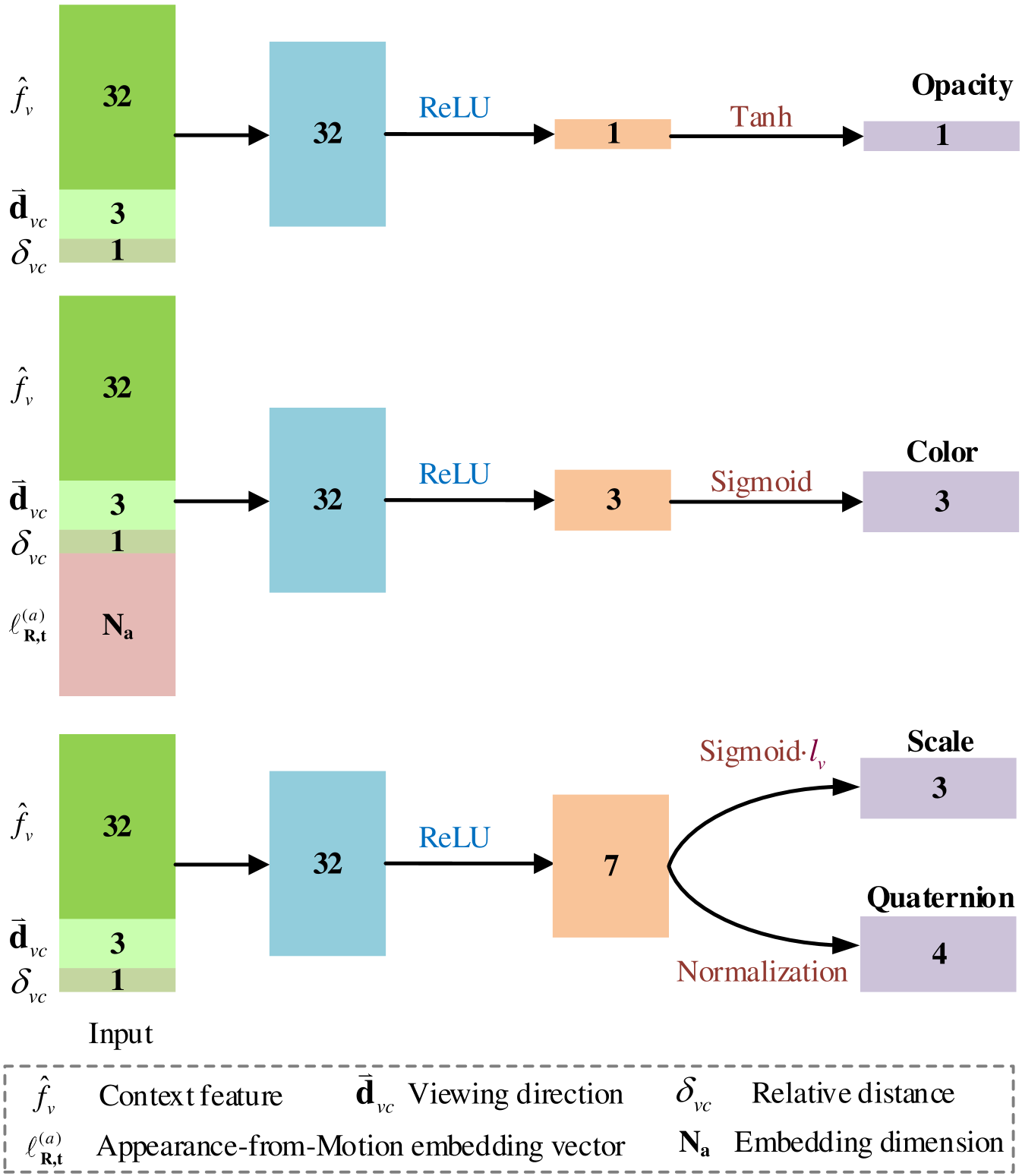
MLPs as feature decoders. Following [21], we employ four MLPs as decoders to derive the parameters of each 3D Gaussian, including the opacity MLP $M_{\alpha}$ , the color MLP $M_{C}$ , and the covariance MLP $M_{q},M_{s}$ . Each MLP adopts a linear layer followed by ReLU and another linear layer. The outputs are activated by their respective activation functions to obtain the final parameters of each 3D Gaussian. The detailed architecture of these MLPs is illustrated in Fig. 11. In our implementation, the hidden layer dimensions of all MLPs are set to 32.

•

For opacity, we use $\mathrm{Tanh(\cdot)}$ to activate the output of the final linear layer. Since the opacity values of 3D Gaussians are typically positive, we constrain the value range to $[0,1)$ to ensure valid outputs.
•

For color, we use $\mathrm{Sigmoid}$ function to activate the output of the final linear layer, which constrains the color value into a range of $[0,1)$ .
•

For rotation, following 3D-GS [15], we employ a normalization to activate the output of the final linear layer, ensuring the validity of the quaternion representation for rotation.
•

For scaling, a $\mathrm{Sigmoid}$ function is applied to activate the output of the final linear layer. Finally, the scaling of each 3D Gaussian is determined by adjusting the scaling $l_{v}$ of its associated anchor based on the MLP’s output, as formulated below:

$\displaystyle\{s_{0},\dots,s_{k-1}\}=M_{s}(\hat{f}_{v},\ \delta_{vc},\ \vec{\mathrm{\mathbf{d}}}_{vc})\cdot l_{v}$ (15)

11.4 Appearance-from-Motion Embedding

MLP as feature encoder. For AfME, we employ an MLP $M_{\theta_{a}}$ as the encoder. The input to this MLP is the camera pose corresponding to each image. The MLP $M_{\theta_{a}}$ extracts pose features and feeds these features to the color decoder $M_{C}$ . The MLP $M_{\theta_{a}}$ adopts a structure of a linear layer followed by a linear activation function, as illustrated in Fig. 12. The entire pipeline for obtaining the Gaussian color is also detailed in Fig. 12. We adopt an encoder-decoder architecture, where an encoder MLP $M_{\theta_{a}}$ extracts features from the camera poses. Unlike FreGS [45], we leverage only high-frequency information, as low-frequency components typically represent scene structure, which is already effectively captured by our structured 3D Gaussians.

Datasets		Replica									TUM RGB-D
Method	Metric	R0	R1	R2	Of0	Of1	Of2	Of3	Of4	Avg.	fr1/d	fr2/x	fr3/o	Avg.
MonoGS [24]	PSNR $\uparrow$	34.29	35.77	36.79	40.87	40.73	35.22	35.89	34.98	36.81	23.59	24.46	24.29	24.11
	SSIM $\uparrow$	0.953	0.957	0.965	0.979	0.977	0.961	0.962	0.955	0.964	0.783	0.789	0.829	0.800
	LPIPS $\downarrow$	0.071	0.078	0.074	0.048	0.052	0.074	0.061	0.092	0.069	0.244	0.227	0.223	0.231
Photo-SLAM [12]	PSNR $\uparrow$	32.09	34.15	35.91	38.70	39.53	33.13	34.15	36.35	35.50	20.14	22.15	20.68	20.99
	SSIM $\uparrow$	0.920	0.941	0.959	0.967	0.964	0.943	0.943	0.956	0.949	0.722	0.765	0.721	0.736
	LPIPS $\downarrow$	0.069	0.055	0.041	0.048	0.045	0.075	0.064	0.053	0.056	0.258	0.169	0.211	0.213
Photo-SLAM-30K	PSNR $\uparrow$	31.41	35.84	38.41	40.44	41.06	34.56	35.43	38.36	36.94	21.78	21.57	21.84	21.73
	SSIM $\uparrow$	0.873	0.955	0.971	0.975	0.972	0.952	0.954	0.967	0.952	0.766	0.755	0.751	0.757
	LPIPS $\downarrow$	0.046	0.036	0.026	0.033	0.033	0.059	0.049	0.036	0.040	0.212	0.182	0.165	0.186
RTG-SLAM [27]	PSNR $\uparrow$	28.49	31.27	32.96	37.32	36.12	31.14	31.19	33.81	32.79	13.62	17.08	18.70	16.47
	SSIM $\uparrow$	0.834	0.902	0.927	0.957	0.943	0.923	0.918	0.937	0.918	0.501	0.573	0.648	0.574
	LPIPS $\downarrow$	0.152	0.119	0.122	0.084	0.103	0.145	0.139	0.125	0.124	0.557	0.403	0.422	0.461
GS-SLAM^∗ [40]	PSNR $\uparrow$	31.56	32.86	32.59	38.70	41.17	32.36	32.03	32.92	34.27	-	-	-	-
	SSIM $\uparrow$	0.968	0.973	0.971	0.986	0.993	0.978	0.970	0.968	0.975	-	-	-	-
	LPIPS $\downarrow$	0.094	0.075	0.093	0.050	0.033	0.094	0.110	0.112	0.082	-	-	-	-
SplaTAM [14]	PSNR $\uparrow$	32.54	33.58	35.03	38.00	38.85	31.71	29.74	31.40	33.85	21.02	23.39	19.81	21.41
	SSIM $\uparrow$	0.938	0.936	0.952	0.963	0.955	0.928	0.902	0.914	0.936	0.753	0.806	0.731	0.764
	LPIPS $\downarrow$	0.068	0.096	0.072	0.087	0.095	0.100	0.119	0.157	0.099	0.341	0.204	0.249	0.265
SGS-SLAM [17]	PSNR $\uparrow$	32.48	33.50	35.11	38.22	38.91	31.86	30.05	31.53	33.96	-	-	-	-
	SSIM $\uparrow$	0.975	0.968	0.983	0.983	0.982	0.966	0.952	0.946	0.969	-	-	-	-
	LPIPS $\downarrow$	0.071	0.099	0.073	0.083	0.091	0.099	0.118	0.154	0.099	-	-	-	-
GS-ICP SLAM [9]	PSNR $\uparrow$	34.89	37.15	37.89	41.62	42.86	32.69	31.45	38.54	37.14	15.67	18.49	19.25	17.81
	SSIM $\uparrow$	0.955	0.965	0.970	0.981	0.981	0.965	0.959	0.969	0.968	0.574	0.667	0.692	0.642
	LPIPS $\downarrow$	0.048	0.045	0.047	0.027	0.031	0.057	0.057	0.045	0.045	0.444	0.308	0.329	0.361
Ours	PSNR $\uparrow$	37.07	39.54	40.33	42.04	43.21	36.38	37.18	39.62	39.42	25.29	26.35	26.46	26.03
	SSIM $\uparrow$	0.968	0.977	0.980	0.982	0.979	0.967	0.969	0.977	0.975	0.839	0.831	0.859	0.843
	LPIPS $\downarrow$	0.023	0.016	0.015	0.020	0.019	0.035	0.026	0.018	0.021	0.136	0.081	0.105	0.107

Table 9: Quantitative evaluation of our method compared to state-of-the-art methods for RGB-D camera on Replica and TUM RGB-D datasets. The best results are marked as best score, second best score and third best score. GS-SLAM^∗ denotes the result of GS-SLAM taken from [40], and all others are obtained in our experiments. ’-’ denotes that the system does not provide valid results.

Datasets (Camera)		Replica (Mono)									TUM RGB-D (Mono)
Method	Metric	R0	R1	R2	Of0	Of1	Of2	Of3	Of4	Avg.	fr1/d	fr2/x	fr3/o	Avg.
MonoGS [24]	PSNR $\uparrow$	26.19	25.42	27.83	31.90	34.22	26.09	28.56	26.49	28.34	20.38	21.21	21.41	21.00
	SSIM $\uparrow$	0.819	0.798	0.889	0.911	0.930	0.881	0.898	0.897	0.878	0.691	0.690	0.735	0.705
	LPIPS $\downarrow$	0.246	0.368	0.252	0.249	0.192	0.268	0.189	0.284	0.256	0.377	0.377	0.426	0.393
Photo-SLAM [12]	PSNR $\uparrow$	30.43	32.11	32.89	37.24	38.10	31.60	32.27	34.16	33.60	19.56	20.82	20.12	20.17
	SSIM $\uparrow$	0.890	0.926	0.937	0.960	0.955	0.932	0.928	0.943	0.934	0.705	0.718	0.702	0.708
	LPIPS $\downarrow$	0.099	0.073	0.069	0.062	0.061	0.094	0.084	0.073	0.077	0.281	0.158	0.233	0.224
Photo-SLAM-30K	PSNR $\uparrow$	32.13	33.14	37.27	38.04	41.73	35.22	34.88	36.22	36.08	22.57	20.54	20.08	21.06
	SSIM $\uparrow$	0.896	0.921	0.965	0.964	0.974	0.952	0.949	0.955	0.947	0.787	0.714	0.697	0.733
	LPIPS $\downarrow$	0.056	0.086	0.035	0.055	0.033	0.061	0.057	0.052	0.054	0.179	0.166	0.213	0.186
Ours	PSNR $\uparrow$	34.94	37.96	38.28	41.19	42.23	36.30	35.44	37.33	37.96	23.94	25.39	26.17	25.17
	SSIM $\uparrow$	0.949	0.967	0.971	0.978	0.972	0.964	0.952	0.959	0.964	0.804	0.813	0.857	0.825
	LPIPS $\downarrow$	0.039	0.027	0.026	0.027	0.036	0.038	0.055	0.050	0.037	0.135	0.121	0.110	0.122

Table 10: Quantitative evaluation of our method compared to state-of-the-art methods for Monocular (Mono) camera on Replica and TUM RGB-D datasets. The best results are marked as best score and second best score.

Datasets		Replica									TUM RGB-D
Method	Metric	R0	R1	R2	Of0	Of1	Of2	Of3	Of4	Avg.	fr1/d	fr2/x	fr3/o	Avg.
ORB-SLAM3 [3]	RMSE $\downarrow$	0.500	0.537	0.731	0.762	1.338	0.636	0.419	9.319	1.780	5.056	0.390	1.143	2.196
DRIOD-SLAM [35]	RMSE $\downarrow$	95.994	52.471	62.908	54.807	36.038	118.191	94.200	79.510	74.264	36.057	16.749	169.844	74.216
MonoGS [24]	RMSE $\downarrow$	0.444	0.273	0.274	0.442	0.469	0.220	0.159	2.237	0.565	1.531	1.440	1.535	1.502
Photo-SLAM [12]	RMSE $\downarrow$	0.529	0.397	0.295	0.501	0.379	1.202	0.768	0.585	0.582	3.578	0.337	1.696	1.870
RTG-SLAM [27]	RMSE $\downarrow$	0.222	0.258	0.248	0.201	0.190	0.115	0.156	0.136	0.191	1.582	0.377	0.996	0.985
GS-SLAM^∗ [40]	RMSE $\downarrow$	0.480	0.530	0.330	0.520	0.410	0.590	0.460	0.700	0.500	3.300	1.300	6.600	3.700
SplaTAM [14]	RMSE $\downarrow$	0.501	0.220	0.298	0.316	0.582	0.256	0.288	0.279	0.343	5.102	1.339	3.329	4.215
SGS-SLAM [17]	RMSE $\downarrow$	0.463	0.216	0.300	0.339	0.547	0.299	0.451	0.311	0.365	-	-	-	-
GS-ICP SLAM [9]	RMSE $\downarrow$	0.189	0.132	0.216	0.201	0.236	0.160	0.162	0.117	0.177	3.539	2.251	2.972	2.921
Ours	RMSE $\downarrow$	0.296	0.264	0.182	0.429	0.354	1.040	0.434	0.441	0.430	3.187	0.370	1.026	1.528

Table 11: Camera tracking result on Replica and TUM RGB-D datasets for RGB-D camera. RMSE of ATE (cm) is reported. The best results are marked as best score, second best score and third best score. ’-’ denotes the system does not provide valid results.

Datasets (Camera)		Replica (Mono)									TUM RGB-D (Mono)
Method	Metric	R0	R1	R2	Of0	Of1	Of2	Of3	Of4	Avg.	fr1/d	fr2/x	fr3/o	Avg.
ORB-SLAM3 [3]	RMSE $\downarrow$	51.388	26.384	4.330	110.212	103.948	65.359	51.145	1.188	51.744	4.3269	10.4598	123.226	46.004
DRIOD-SLAM [35]	RMSE $\downarrow$	103.892	53.146	66.939	53.267	34.431	119.311	98.089	83.732	76.600	1.769	0.458	2.839	1.689
MonoGS [24]	RMSE $\downarrow$	12.623	56.357	25.350	43.245	19.729	39.148	11.754	88.230	37.054	4.575	4.605	2.847	4.009
Photo-SLAM [12]	RMSE $\downarrow$	0.336	0.551	0.234	2.703	0.505	2.065	0.399	0.644	0.930	1.633	0.935	2.050	1.539
Ours	RMSE $\downarrow$	0.288	0.388	0.215	0.579	0.320	3.963	0.307	0.603	0.833	3.187	0.370	1.026	1.505

Table 12: Camera tracking result on Replica and TUM RGB-D datasets for monocular camera. RMSE of ATE (cm) is reported. Best results are marked as best score, second best score and third best score.

11.5 Anchor Points Refinement

Our anchor refinement strategy follows [21], and it is included here to enhance the completeness of this paper.

Anchor Growing. 3D Gaussians are spatially quantized into voxels of size $\epsilon_{g}=0.001$ . For all 3D Gaussians within each voxel, we compute the average gradient after $N_{t}=100$ training iterations, denoted as $\nabla_{g}$ . When the average gradient $\nabla_{g}$ within a voxel exceeds a threshold $\tau_{g}=0.0002$ , a new anchor is added at the center of the voxel. Since the total loss includes the frequency regularization $\mathcal{L}_{hf}$ in Eq. 9, anchor points grow toward underrepresented high-frequency regions in the scene. Ultimately, the local details of the scene are refined. In our implementation, the scene is quantized into a multi-resolution voxel grid, allowing new anchors to be added to regions of varying sizes, as defined by

\displaystyle\epsilon_{g}^{(m)}=\epsilon_{g}/4^{m-1},\ \tau_{g}^{(m)}=\tau_{g}\cdot 2^{m-1}

(16)

where $m$ denotes the level of quantization. Additionally, we adopt a random candidate pruning strategy to moderate the growth rate of anchors.

To eliminate redundant anchor points, we evaluate their opacity. Specifically, after $N_{t}$ training iterations, we accumulate the opacity values of each 3D Gaussian. If the accumulated value $\alpha_{p}$ falls below a pre-defined threshold, the Gaussian is removed from the scene.

11.6 Experimental Parameters

For the monocular camera in the Replica dataset, the dimension of AfME $N_{a}$ is set to 1, while for other configurations, it is set to $32$ . Each anchor manages $k=10$ 3D Gaussians. Anchors with an opacity value below $0.005$ are removed. The loss weights $\lambda$ , $\lambda_{\text{vol}}$ , and $\lambda_{hf}$ are set to $0.2$ , $0.01$ , and $0.01$ , respectively. For the monocular camera in the Replica dataset, the weight $\lambda_{hf}$ for frequency regularization is set to $0.025$ , and the frequency pyramid consists of $3$ levels.

12 Additional Qualitative Results

12.1 Per-scene Results.

Tab. 9, Tab. 10, Tab. 13(a), Tab. 11, Tab. 12, and Tab. 13(b) present the photorealistic mapping and localization results of our method across all datasets for each scene. Additionally, Fig. 13, Fig. 14, Fig. 15, Fig. 16, and Fig. 17 show more rendering comparisons between our method and all baseline methods for each scene.

Datasets (Camera)		EuRoC (Stereo)
Method	Metric	MH01	MH02	V101	V201	Avg.
MonoGS	PSNR $\uparrow$	22.84	25.53	23.39	18.66	22.60
[24]	SSIM $\uparrow$	0.789	0.850	0.831	0.687	0.789
	LPIPS $\downarrow$	0.243	0.181	0.287	0.384	0.274
Photo-	PSNR $\uparrow$	11.22	11.14	13.78	11.46	11.90
SLAM	SSIM $\uparrow$	0.300	0.306	0.520	0.509	0.409
[12]	LPIPS $\downarrow$	0.469	0.464	0.394	0.427	0.439
Photo-	PSNR $\uparrow$	11.10	11.04	13.66	11.26	11.77
SLAM-	SSIM $\uparrow$	0.296	0.300	0.516	0.508	0.405
30K	LPIPS $\downarrow$	0.466	0.457	0.389	0.409	0.430
Ours	PSNR $\uparrow$	22.50	22.30	24.90	24.89	23.64
	SSIM $\uparrow$	0.750	0.727	0.843	0.842	0.791
	LPIPS $\downarrow$	0.220	0.269	0.122	0.117	0.182

(a) Quantitative evaluation of our method compared to state-of-the-art methods for Stereo camera on EuRoC MAV datasets. The best results are marked as best score and second best score.

Datasets (Camera)		EuRoC (Stereo)
Method	Metric	MH01	MH02	V101	V201	Avg.
ORB-SLAM3 [3]	RMSE $\downarrow$	4.806	4.938	8.829	25.057	10.907
DRIOD-SLAM [35]	RMSE $\downarrow$	1.177	1.169	3.678	1.680	1.926
MonoGS [24]	RMSE $\downarrow$	11.194	8.327	29.365	148.080	49.241
Photo-SLAM [12]	RMSE $\downarrow$	3.997	4.547	8.882	26.665	11.023
Ours	RMSE $\downarrow$	3.948	3.863	8.823	13.217	7.462

(b) Camera tracking result on EuRoC MAV datasets for stereo camera. RMSE of ATE (cm) is reported. The best results are marked as best score and second best score.

Table 13: Quantitative evaluation of our method compared to state-of-the-art methods for Stereo camera on EuRoC MAV datasets.