Selective Ensembling for Prediction Consistency

Appendix A Proofs

A.1 Proof of Theorem 3.1

Refer to caption — Figure 1: Intuitive illustration of how two models which predict identical classification labels can have arbitrary gradients. To show this, given a binary classifier $H$ and an arbitrary function $g$ , we construct a classifier $H^{\prime}$ that predicts the same labels as $H$ , yet has gradients equal to $g$ almost everywhere. We formally state this result in Theorem A.1.

Theorem 3.1.

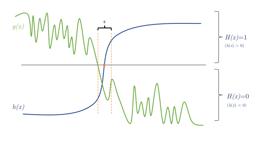
Let $H:\mathbf{X}\rightarrow\{-1,1\}=\mathrm{sign}(h)$ be a binary classifier and $g:\mathbf{X}\rightarrow\mathbb{R}$ be an unrelated function that is bounded from above and below, continuous, and piecewise differentiable. Then there exists another binary classifier $\hat{H}=\mathrm{sign}(\hat{h})$ such that for any $\epsilon>0$ ,

\forall x\in\mathbf{X}~{}.\hskip 20.00003pt\text{1.}~{}~{}\hat{H}(x)=H(x)\hskip 20.00003pt\text{2.}~{}~{}\inf_{x^{\prime}:H(x^{\prime})\neq H(x)}\Big{\{}||x-x^{\prime}||\Big{\}}>\nicefrac{{\epsilon}}{{2}}~{}~{}\Longrightarrow~{}~{}\nabla\hat{h}(x)=\nabla g(x)

Proof.

We partition $\mathbf{X}$ into regions $\{I_{1}....I_{k}\}$ determined by the decision boundaries of $H$ . That is, each $I_{i}$ represents a maximal contiguous region for which each $x\in I_{i}$ receives the same label from $H$ .

Recall we are given a function $g:\mathbf{X}\rightarrow\mathbb{R}$ which is bounded from above and below. We create a set of functions $\hat{g_{I_{i}}}:I_{i}\rightarrow R$ such that

\hat{g}_{I_{i}}(x)=\begin{cases}g(x)-\inf_{x}g(x)+c&\text{ if $H(I_{i})=1$}\\ g(x)-\sup_{x}g(x)-c&\text{ if $H(I_{i})=-1$}\end{cases}

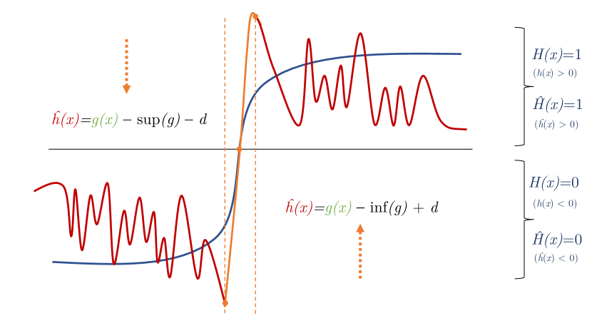
where $c$ is some small constant greater than zero. Additionally, let $d(x)$ be the $\ell_{2}$ distance from $x$ to the nearest decision boundary of $h$ , i.e. $d(x)=\inf_{x^{\prime}:H(x^{\prime})\neq H(x)}\Big{\{}||x-x^{\prime}||\Big{\}}$ . Then, we define $\hat{h}$ to be:

\hat{h}(x)=\begin{cases}\hat{g}_{I_{i}}(x)&\text{ for $x$ }\in I_{i}\text{ if $d(x)>\frac{\epsilon}{2}$}\\ \hat{g}_{I_{i}}(x)\cdot\frac{2d(x)}{\epsilon}&\text{ for $x$ }\in I_{i}\text{ if $d(x)\leq\frac{\epsilon}{2}$}\\ \end{cases}

And, as described above, we define $\hat{H}=\text{sign}(\hat{h})$ . First, we show that $\hat{H}(x)=H(x)~{}~{}\forall x\in\mathbf{X}$ . Without loss of generality, consider some $I_{i}$ where $H(x)=1$ , for any $x\in I_{i}$ . We first consider the case where $d(x)>\frac{\epsilon}{2}$ .

By construction, for $x\in I_{i}$ , $\hat{H}(x)=\text{sign}(\hat{h}(x))=\text{sign}(\hat{g}_{I_{i}}(x))=\text{sign}(g(x)-\inf_{x}g(x)+c)$ . By definition of the infimum, $g(x)-\inf_{x}g(x)\geq 0$ , and thus $\text{sign}(g(x)-\inf_{x}g(x)+c)=1$ , so $\hat{H}(x)=1=H(x)$ .

Note that in the case where $d(x)\leq\frac{\epsilon}{2}$ , we can follow the same argument as multiplication by a positive constant does not affect the sign. A symmetric argument follows for the case where for $x\in I_{i}$ , $H(x)=-1$ ; thus, $\hat{H}(x)=H(x)~{}~{}\forall x\in\mathbf{X}$ .

Secondly, we show that $\nabla\hat{h}(x)=\nabla g(x)~{}~{}\forall x$ where $d(x)>\frac{\epsilon}{2}$ . Consider the case where $H(x)=1$ . By construction, $\hat{h}(x)=\hat{g}_{I_{i}}(x)=g(x)-\inf_{x}g(x)+c$ . Note that this means the infimum and $c$ are constants, so their gradients are zero. Thus, $\nabla\hat{h}(x)=\nabla g(x)$ . A symmetric argument holds for the case where $H(x)=-1$ .

It remains to prove that $\hat{h}$ is continuous and piecewise differentiable, in order to be a realizable as a ReLU-network. By assumption, $g$ is piecewise differentiable, which means that $\hat{g_{i}}$ are piecewise differentiable as well, as is $\hat{g_{i}}(x)\cdot\frac{d(x)}{\epsilon}$ . Thus, $\hat{h}$ is piecewise-differentiable. To see that $\hat{h}$ is continuous, consider the case where $d(x)=\nicefrac{{\epsilon}}{{2}}$ for some $x$ . Then $\hat{g_{i}}(x)\cdot\frac{d(x)}{\epsilon}=\hat{g_{i}}(x)\cdot\frac{\epsilon}{\epsilon}=\hat{g_{i}}(x)$ . Additionally, consider the case where $d(x)=0$ , i.e. $x$ is on a decision boundary of $h(x)$ , between two regions $I_{i},I_{j}$ . Then $\hat{h}(x)=\hat{g_{i}}(x)\cdot\frac{d(x)}{\epsilon}=\hat{g_{i}}(x)\cdot 0=0=\hat{g_{j}}(x)\cdot 0=\hat{g_{j}}(x)$ . This shows that the piecewise components of $\hat{h}$ come to the same value at their intersection.Further, each piecewise component of $\hat{h}$ is equal to some continuous function, as $g(x)$ is continuous by assumption. Thus, $\hat{h}$ is continuous, and we conclude our proof. ∎

We include a visual intuition of the proof in Figure 1.

A.2 Proof of Theorem 4.1

Theorem 4.1.

Let $\mathcal{P}$ be a learning pipeline, and let $\mathcal{S}$ be a distribution over random states. Further, let $g_{\mathcal{P},\mathcal{S}}$ be the mode predictor, let $\hat{g}_{n}(\mathcal{P},S)$ for $S\sim\mathcal{S}^{n}$ be a selective ensemble, and let $\alpha\geq 0$ . Then,

\forall x\in\mathbf{X}~{}~{}.~{}~{}\mathop{\mathbf{Pr}}_{S\sim\mathcal{S}^{n}}\Big{[}\hat{g}_{n}(\mathcal{P},S~{};~{}\alpha,x)\mathrel{\mathop{\neq}\limits^{\vbox to-1.39998pt{\kern-2.0pt\hbox{${}_{\mathtt{ABS}}$}\vss}}}g_{\mathcal{P},\mathcal{S}}(x)\Big{]}\leq\alpha

Proof.

$\hat{g}_{n}(\mathcal{P},S)$ is an ensemble of $n$ models. By the definition of Algorithm LABEL:prediction_algo, $\hat{g}_{n}(\mathcal{P},S)$ gathers a vector of class counts of the prediction for $x$ from each model in the ensemble. Let the class with the highest count be $c_{A}$ , with counts $n_{A}$ , and the class with the second highest count be called $c_{B}$ , with counts $n_{B}$ . $\hat{g}_{n}(\mathcal{P},S)$ runs a two-sided hypothesis test to ensure that $\Pr[n_{A}\sim\text{Binomial}(n_{A}+n_{B},0.5)]<\alpha$ , i.e. that $c_{A}$ is the true mode prediction over $\mathcal{S}$ . See that

	$\displaystyle\Pr\Big{[}g_{\mathcal{P},\mathcal{S}}(x)\neq c_{A}~{}~{}\land~{}~{}\hat{g}_{n}(\mathcal{P},S~{};~{}\alpha,x)=c_{A}\Big{]}$		(1)
$\displaystyle=~{}$	$\displaystyle\Pr\Big{[}g_{\mathcal{P},\mathcal{S}}(x)\neq c_{A}\Big{]}\cdot\Pr\Big{[}\hat{g}_{n}(\mathcal{P},S~{};~{}\alpha,x)\neq\mathtt{ABSTAIN}~{}\|~{}g_{\mathcal{P},\mathcal{S}}(x)\neq c_{A}\Big{]}$		(2)
$\displaystyle\leq~{}$	$\displaystyle\Pr\Big{[}\hat{g}_{n}(\mathcal{P},S~{};~{}\alpha,x)\neq\mathtt{ABSTAIN}~{}\|~{}g_{\mathcal{P},\mathcal{S}}(x)\neq c_{A}\Big{]}$		(3)
$\displaystyle\leq~{}$	$\displaystyle\Pr\Big{[}\hat{g}_{n}(\mathcal{P},S~{};~{}\alpha,x)\neq\mathtt{ABSTAIN}~{}\|~{}g_{\mathcal{P},\mathcal{S}}(x)\neq c_{A}\Big{]}=\alpha$	By hung2019rank	(4)

Thus,

\Pr\Big{[}g_{\mathcal{P},\mathcal{S}}(x)\neq c_{A}~{}~{}\land~{}~{}\hat{g}_{n}(\mathcal{P},S~{};~{}\alpha,x)=c_{A}\Big{]}\leq\alpha

∎

A.3 Proof of Corollary 4.2

Corollary 4.2.

Let $\mathcal{P}$ be a learning pipeline, and let $\mathcal{S}$ be a distribution over random states. Further, let $g_{\mathcal{P},\mathcal{S}}$ be the mode predictor, let $\hat{g}_{n}(\mathcal{P},S)$ for $S\sim\mathcal{S}^{n}$ be a selective ensemble. Finally, let $\alpha\geq 0$ , and let $\beta\geq 0$ be an upper bound on the expected abstention rate of $\hat{g}_{n}(\mathcal{P},S)$ . Then, the expected loss variance, $V(x)$ , over inputs, $x$ , is bounded by $\alpha+\beta$ . That is,

\mathop{\mathbb{E}}_{x\sim\mathcal{D}}\Big{[}V(x)\Big{]}=\mathop{\mathbb{E}}_{x\sim\mathcal{D}}\Bigg{[}~{}\Pr_{S\sim\mathcal{S}^{n}}\Big{[}\hat{g}_{n}(\mathcal{P},S~{};~{}x)\neq g_{\mathcal{P},\mathcal{S}}(x)\Big{]}~{}\Bigg{]}\leq\alpha+\beta

Proof.

Since $g_{\mathcal{P},\mathcal{S}}$ never abstains, we have by the law of total probability that

	$\displaystyle\Pr_{S\sim\mathcal{S}^{n}}\Big{[}\hat{g}_{n}(\mathcal{P},S~{};~{}\alpha,x)\neq g_{\mathcal{P},\mathcal{S}}(x)\Big{]}$	$\displaystyle=\Pr_{S\sim\mathcal{S}^{n}}\Big{[}\hat{g}_{n}(\mathcal{P},S~{};~{}\alpha,x)\mathrel{\mathop{\neq}\limits^{\vbox to-1.11998pt{\kern-2.0pt\hbox{${}_{\mathtt{ABS}}$}\vss}}}g_{\mathcal{P},\mathcal{S}}(x)~{}~{}\lor~{}~{}\hat{g}_{n}(\mathcal{P},S~{};~{}\alpha,x)=\mathtt{ABSTAIN}$
		$\displaystyle=\Pr_{S\sim\mathcal{S}^{n}}\Big{[}\hat{g}_{n}(\mathcal{P},S~{};~{}\alpha,x)\mathrel{\mathop{\neq}\limits^{\vbox to-1.11998pt{\kern-2.0pt\hbox{${}_{\mathtt{ABS}}$}\vss}}}g_{\mathcal{P},\mathcal{S}}(x)\Big{]}+\Pr_{S\sim\mathcal{S}^{n}}\Big{[}\hat{g}_{n}(\mathcal{P},S~{};~{}\alpha,x)=\mathtt{ABSTAIN}\Big{]}$

By Theorem LABEL:thm:matches_mode, we have that $\Pr_{S\sim\mathcal{S}^{n}}\big{[}\hat{g}_{n}(\mathcal{P},S~{};~{}\alpha,x)\mathrel{\mathop{\neq}\limits^{\vbox to-1.39998pt{\kern-2.0pt\hbox{${}_{\mathtt{ABS}}$}\vss}}}g_{\mathcal{P},\mathcal{S}}(x)\big{]}\leq\alpha$ , thus

\mathop{\mathbb{E}}_{x\sim\mathcal{D}}\Bigg{[}~{}\Pr_{S\sim\mathcal{S}^{n}}\Big{[}\hat{g}_{n}(\mathcal{P},S~{};~{}\alpha,x)\neq g_{\mathcal{P},\mathcal{S}}(x)\Big{]}~{}\Bigg{]}\leq\alpha+\mathop{\mathbb{E}}_{x\sim\mathcal{D}}\Bigg{[}~{}\Pr_{S\sim\mathcal{S}^{n}}\Big{[}\hat{g}_{n}(\mathcal{P},S~{};~{}\alpha,x)=\mathtt{ABSTAIN}\Big{]}~{}\Bigg{]}

Finally, since $\beta$ is an upper bound on the expected abstention rate of $\hat{g}_{n}(\mathcal{P},S)$ , we conclude that

\mathop{\mathbb{E}}_{x\sim\mathcal{D}}\Bigg{[}~{}\Pr_{S\sim\mathcal{S}^{n}}\Big{[}\hat{g}_{n}(\mathcal{P},S~{};~{}\alpha,x)\neq g_{\mathcal{P},\mathcal{S}}(x)\Big{]}~{}\Bigg{]}\leq\alpha+\beta

∎

A.4 Proof of Corollary 4.3

Corollary 4.3.

Let $\mathcal{P}$ be a learning pipeline, and let $\mathcal{S}$ be a distribution over random states. Further, let $\hat{g}_{n}(\mathcal{P},S)$ for $S\sim\mathcal{S}^{n}$ be a selective ensemble. Finally, let $\alpha\geq 0$ , and let $\beta\geq 0$ be an upper bound on the expected abstention rate of $\hat{g}_{n}(\mathcal{P},S)$ . Then,

\mathop{\mathbb{E}}_{x\sim\mathcal{D}}\Bigg{[}~{}\mathop{\mathbf{Pr}}_{S^{1},S^{2}\sim\mathcal{S}^{n}}\Big{[}\hat{g}_{n}(\mathcal{P},S^{1}~{};~{}\alpha,x)\neq\hat{g}_{n}(\mathcal{P},S^{2}~{};~{}\alpha,x)\Big{]}~{}\Bigg{]}\leq 2(\alpha+\beta)

Proof.

For $i\in\{1,2\}$ , let $A^{i}$ be the event that $\hat{g}_{n}(\mathcal{P},S^{i}~{};~{}\alpha,x)=\mathtt{ABSTAIN}$ , and let $N^{i}$ be the event that $\hat{g}_{n}(\mathcal{P},S^{i}~{};~{}\alpha,x)\mathrel{\mathop{\neq}\limits^{\vbox to-1.39998pt{\kern-2.0pt\hbox{${}_{\mathtt{ABS}}$}\vss}}}g_{\mathcal{P},\mathcal{S}}$ . In the worst case, $A^{1}$ and $A^{2}$ , and $N^{1}$ and $N^{2}$ are disjoint, that is, e.g., if $\hat{g}_{n}(\mathcal{P},S^{i})$ abstains on $x$ , then $\hat{g}_{n}(\mathcal{P},S^{1}~{};~{}\alpha,x)\neq\hat{g}_{n}(\mathcal{P},S^{2}~{};~{}\alpha,x)$ . In other words, we have that

\mathop{\mathbf{Pr}}_{S^{1},S^{2}\sim\mathcal{S}^{n}}\Big{[}\hat{g}_{n}(\mathcal{P},S^{1}~{};~{}\alpha,x)\neq\hat{g}_{n}(\mathcal{P},S^{2}~{};~{}\alpha,x)\Big{]}\leq\mathop{\mathbf{Pr}}\Big{[}A^{1}~{}\lor~{}A^{2}~{}\lor~{}N^{1}~{}\lor~{}N^{2}\Big{]}

which, by union bound implies that

\mathop{\mathbf{Pr}}_{S^{1},S^{2}\sim\mathcal{S}^{n}}\Big{[}\hat{g}_{n}(\mathcal{P},S^{1}~{};~{}\alpha,x)\neq\hat{g}_{n}(\mathcal{P},S^{2}~{};~{}\alpha,x)\Big{]}\leq\mathop{\mathbf{Pr}}\big{[}A^{1}\big{]}+\mathop{\mathbf{Pr}}\big{[}A^{2}\big{]}+\mathop{\mathbf{Pr}}\big{[}N^{1}\big{]}+\mathop{\mathbf{Pr}}\big{[}N^{2}\big{]}.

By Theorem LABEL:thm:matches_mode $\Pr\big{[}N^{i}\big{]}\leq\alpha$ . Thus we have

\mathop{\mathbb{E}}_{x\sim\mathcal{D}}\Bigg{[}~{}\mathop{\mathbf{Pr}}_{S^{1},S^{2}\sim\mathcal{S}^{n}}\Big{[}\hat{g}_{n}(\mathcal{P},S^{1}~{};~{}\alpha,x)\neq\hat{g}_{n}(\mathcal{P},S^{2}~{};~{}\alpha,x)\Big{]}~{}\Bigg{]}\leq 2\alpha+\mathop{\mathbb{E}}_{x\sim\mathcal{D}}\Big{[}~{}\mathop{\mathbf{Pr}}\big{[}A^{1}\big{]}~{}\Big{]}+\mathop{\mathbb{E}}_{x\sim\mathcal{D}}\Big{[}~{}\mathop{\mathbf{Pr}}\big{[}A^{2}\big{]}~{}\Big{]}.

Finally, since $\beta$ is an upper bound on the expected abstention rate of $\hat{g}_{n}(\mathcal{P},S)$ , we conclude that

\mathop{\mathbb{E}}_{x\sim\mathcal{D}}\Bigg{[}~{}\mathop{\mathbf{Pr}}_{S^{1},S^{2}\sim\mathcal{S}^{n}}\Big{[}\hat{g}_{n}(\mathcal{P},S^{1}~{};~{}\alpha,x)\neq\hat{g}_{n}(\mathcal{P},S^{2}~{};~{}\alpha,x)\Big{]}~{}\Bigg{]}\leq 2(\alpha+\beta)

∎

Appendix B Datasets

The German Credit and Taiwanese data sets consist of individuals financial data, with a binary response indicating their creditworthiness. For the German Credit dataset, there are 1000 points, and 20 attributes. We one-hot encode the data to get 61 features, and standardize the data to zero mean and unit variance using SKLearn Standard scaler. We partitioned the data intro a training set of 700 and a test set of 200. The Taiwanese credit dataset has 30,000 instances with 24 attributes. We one-hot encode the data to get 32 features and normalize the data to be between zero and one. We partitioned the data intro a training set of 22500 and a test set of 7500.

The Adult dataset consists of a subset of publicly-available US Census data, binary response indicating annual income of $>50$ k. There are 14 attributes, which we one-hot encode to get 96 features. We normalize the numerical features to have values between $0$ and $1$ . After removing instances with missing values, there are $30,162$ examples which we split into a training set of 14891, a leave one out set of 100, and a test set of 1501 examples.

The Seizure dataset comprises time-series EEG recordings for 500 individuals, with a binary response indicating the occurrence of a seizure. This is represented as 11500 rows with 178 features each. We split this into 7,950 train points and 3,550 test points. We standardize the numeric features to zero mean and unit variance.

The Warfain dataset is collected by the International Warfarin Pharmacogenetics Consortium [nejm-warfarin] about patients who were prescribed warfarin. We removed rows with missing values, 4819 patients remained in the dataset. The inputs to the model are demographic (age, height, weight, race), medical (use of amiodarone, use of enzyme inducer), and genetic (VKORC1, CYP2C9) attributes. Age, height, and weight are real-valued and were scaled to zero mean and unit variance. The medical attributes take binary values, and the remaining attributes were one-hot encoded. The output is the weekly dose of warfarin in milligrams, which we encode as "low", "medium", or "high", following the recommendations set by nejm-warfarin.

Fashion MNIST contains images of clothing items, with a multilabel response of 10 classes. There are 60000 training examples and 10000 test examples. We pre-process the data by normalizing the numerical values in the image array to be between $0$ and $1$ .

The colorectal histology dataset contains images of human colorectal cancer, with a multilabel response of 8 classes. There are 5,000 images, which we divide into a training set of 3750 and a validation set of 1250. We pre-process the data by normalizing the numerical values in the image array to be between $0$ and $1$ .

The UCI datasets as well as FMNIST are under an MIT license, the colorectal histology and Warfarin datasets are under a Creative Commons License. [uci, colon_license, nejm-warfarin].

Appendix C Model Architecture and Hyper-Parameters

The German Credit and Seizure models have three hidden layers, of size 128, 64, and 16. Models on the Adult dataset have one hidden layer of 200 neurons. Models on the Taiwanese dataset have two hidden layers of 32 and 16. The Warfarin models have one hidden layer of 100. The FMNIST model is a modified LeNet architecture [lecun1995learning]. This model is trained with dropout. The Colon models are trained with a modified, ResNet50 [he2016deep], pre-trained on ImageNet [deng2009imagenet], available from Keras. German Credit, Adult, Seizure, Taiwanese, and Warfarin models are trained for 100 epochs; FMNIST for 50, and Colon models are trained for 20 epochs. German Credit models are trained with a batch size of 32; FMNIST 64; Adult, Seizure, and Warfarin models with batch sizes of 128; and Colon and Taiwanese Credit models with batch sizes of 512. German Credit, Adult, Seizure, Taiwanese Credit, Warfarin, and Colon are trained with keras’ Adam optimizer with the default parameters. FMNIST models are trained with keras’ SGD optimizer with the default parameters.

Note that we discuss train-test splits and data preprocessing above in Section B. We prepare different models for the same dataset using Tensorflow 2.3.0 and all computations are done using a Titan RTX accelerator on a machine with 64 gigabytes of memory.

Appendix D Metrics

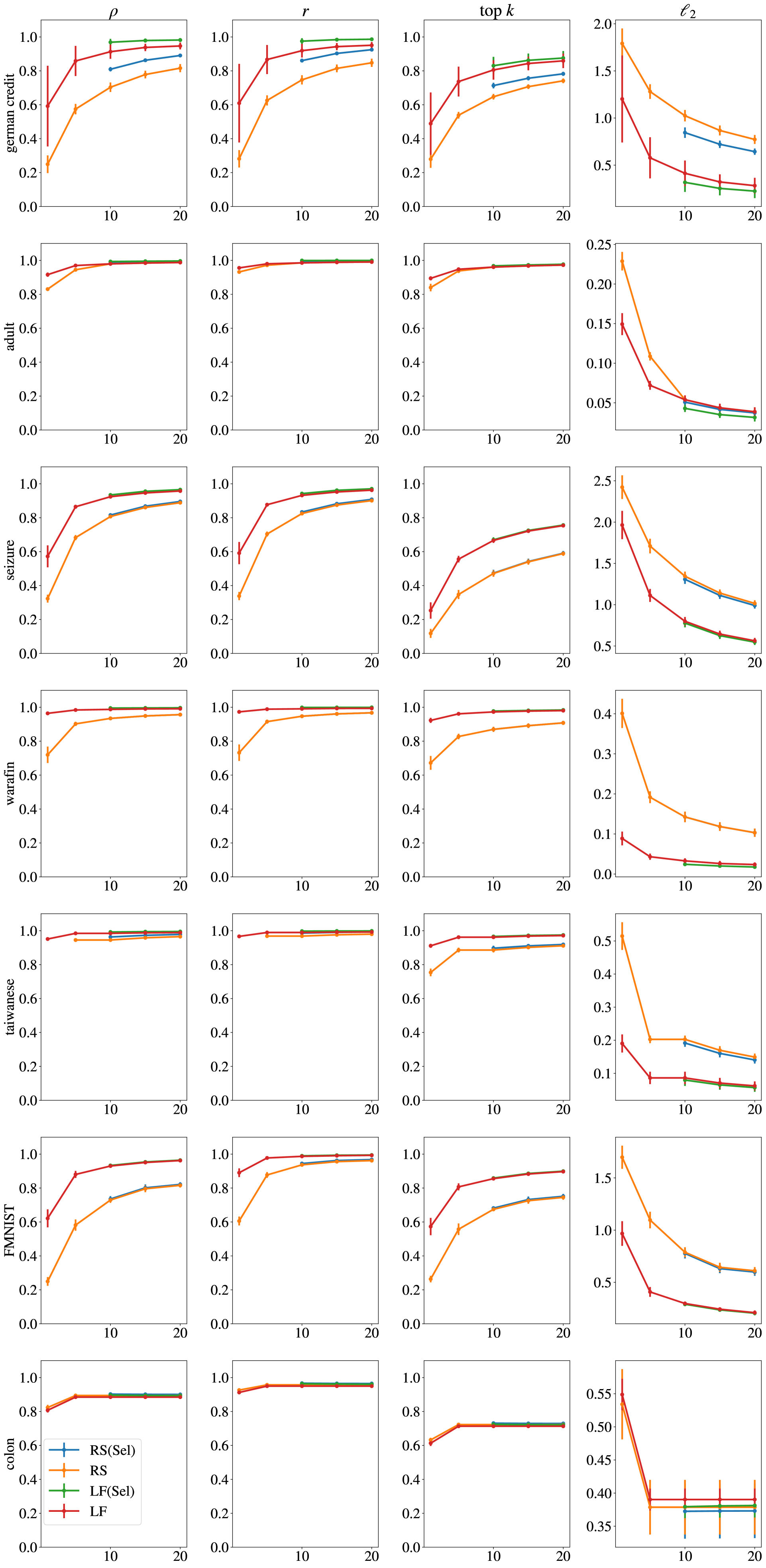
We report similarity between feature attributions with Spearman’s Ranking Correlation ( $\rho$ ), Pearson’s Correlation Coefficient ( $r$ ), top- $k$ intersection, $\ell_{2}$ distance, and SSIM for image datasets. We use standard implementations for Spearman’s Ranking Correlation ( $\rho$ ) and Pearson’s Correlation Coefficient ( $r$ ) from scipy, and implement $\ell_{2}$ distance as well as the top- $k$ using numpy functions.

Note that $r$ and $\rho$ vary from -1 to 1, denoting negative, zero, and positive correlation. We display top- $k$ for $k$ =5, and compute this by taking the number of features in the intersection of the top $5$ between two models, and then diving this by $5$ . Thus top- $k$ is between 0 and 1, indicating low and high correlation respectively.

The $\ell_{2}$ distance has a minimum of $0$ , but is unbounded from above, and SSIM varies from -1 to 1, indicating no correlation to exact correlation respectively.

Note that we compute these metrics between two different models on the same point, for every point in the test set, over 276 different pairs of models for tabular datasets and over 40 pairs of models for image datasets. We average this result over the points in the test set and over the comparisons to get the numbers displayed in the tables and graphs throughout the paper.

D.1 SSIM

Explanations for image models can be interpreted as an image (as there is an attribution for each pixel), and are often evaluated visually [leino18influence, simonyan2014deep, sundararajan2017axiomatic]. However, pixel-wise indicators for similarity between images (such as top-k similarity between pixel values, Spearman’s ranking coefficient, or mean squared error) often do not capture how similar images are visually, in aggregate. In order to give an indication if the entire explanation for an image model, i.e. the explanatory image produced, is similar, we use the structural similarity index (SSIM) [wang2004image]. We use the implementation from $\mathtt{scikit-image}$ [structural_similarity_index]. SSIM varies from -1 to 1, indicating no correlation to exact correlation respectively.

Appendix E Experimental Results for $\alpha=0.01$

We include results on the prediction of selective ensemble models for $\alpha=0.01$ as well. We include the percentage of points with disagreement between at least one pair of models ( $p_{\text{flip}}>0$ ) trained with different random seeds (RS) or leave-one-out differences in training data, for singleton models ( $n=1$ ) and selective ensembles ( $n>1$ ) in Table 1. Notice the number of points with $p_{\text{flip}}>0$ is again zero. We also include the mean and standard deviation of accuracy and abstention rate for $\alpha=0.01$ in Table 2.

mean $\pm$ std. dev of portion of test data with $p_{\text{flip}}>0$
Randomness	$n$	Ger. Credit	Adult	Seizure	Tai. Credit	Warfarin	FMNIST	Colon
RS	1	$.570\pm.020$	$.087\pm.001$	$.060\pm.01$	$.082\pm.002$	$.098\pm.003$	$.061\pm.008$	$.037\pm.005$
RS	(5, 10, 15, 20)	$0.0\pm 0.0$	$0.0\pm 0.0$	$0.0\pm 0.0$	$0.0\pm 0.0$	$0.0\pm 0.0$	$0.0\pm 0.0$	$0.0\pm 0.0$
LOO	1	$.262\pm.014$	$.063\pm.001$	$.031\pm.001$	$.031\pm.001$	$.033\pm.003$	$.034\pm.004$	$.042\pm.005$
LOO	(5, 10, 15, 20)	$0.0\pm 0.0$	$0.0\pm 0.0$	$0.0\pm 0.0$	$0.0\pm 0.0$	$0.0\pm 0.0$	$0.0\pm 0.0$	$0.0\pm 0.0$

Table 1: The percentage of points with disagreement between at least one pair of models (

p_{\text{flip}}>0

) trained with different random seeds (RS) or leave-one-out differences in training data, for singleton models (

n=1

) and selective ensembles (

n>1

). Results for selective ensembles all selective ensembles are shown together, as they all have no disagreement. Note that these results are for

\alpha=0.01

. But this different

\alpha

also leads to zero disagreement between predicted points.

	mean accuracy (abstain as error) / std. dev
$\mathcal{S}$	$n$	Ger. Credit	Adult	Seizure	Wafarin	Tai. Credit	FMNIST	Colon
RS	5	$0.0\pm 0.0$	$0.0\pm 0.0$	$0.0\pm 0.0$	$0.0\pm 0.0$	$0.0\pm 0.0$	$0.0\pm 0.0$	$0.0\pm 0.0$
RS	10	$.461\pm.016$	$.807\pm 1e-3~{}$	$.945\pm 2e-3$	$.646\pm 3e-3$	$.788\pm 2e-3$	$.870\pm 5e-3$	$.902\pm 2e-3$
RS	15	$.589\pm.015$	$.822\pm 8e-4~{}$	$.961\pm 1e-3$	$.661\pm 3e-3$	$.802\pm 9e-4$	$.890\pm 2e-3$	$.915\pm 1e-3$
RS	20	$.593\pm.011$	$.822\pm 7e-4~{}$	$.961\pm 8e-4$	$.662\pm 1e-3$	$.803\pm 9e-4$	$.991\pm 1e-3$	$.926\pm 1e-3$
LOO	5	$0.0\pm 0.0$	$0.0\pm 0.0$	$0.0\pm 0.0$	$0.0\pm 0.0$	$0.0\pm 0.0$	$0.0\pm 0.0$	$0.0\pm 0.0$
LOO	10	$.618\pm.017$	$.818\pm 1e-3$	$.947\pm 4e-3$	$.674\pm 2e-3$	$.807\pm 1e-3$	$.904\pm 6e-4$	$.901\pm 2e-3$
LOO	15	$.656\pm.017$	$.828\pm 1e-3~{}$	$.963\pm 1e-3$	$.678\pm 9e-4$	$.812\pm 9e-4$	$.908\pm 1e-3$	$.912\pm 2e-3$
LOO	20	$.661\pm.018$	$.829\pm 7e-4~{}$	$.964\pm 1e-3$	$.678\pm 7e-4$	$.812\pm 8e-4$	$.909\pm 6e-4$	$.912\pm 2e-3$
	mean abstention rate / std dev
$\mathcal{S}$	$n$	Ger. Credit	Adult	Seizure	Warfarin	Tai. Credit	FMNIST	Colon
RS	5	$1.0\pm 0.0$	$1.0\pm 0.0$	$1.0\pm 0.0$	$1.0\pm 0.0$	$1.0\pm 0.0$	$1.0\pm 0.0$	$1.0\pm 0.0$
RS	10	$.449\pm.021$	$.068\pm 2e-3$	$.045\pm 2e-3$	$.078\pm 5e-3$	$.063\pm 2e-3$	$.087\pm 8e-3$	$.050\pm 3e-3$
RS	15	$.278\pm.017$	$.041\pm 1e-3$	$.025\pm 1e-3$	$.049\pm 3e-3$	$.037\pm 1e-3$	$.055\pm 2e-3$	$.030\pm 2e-3$
RS	20	$.270\pm.015$	$.040\pm 1-e3$	$.024\pm 1e-3$	$.047\pm 2e-3$	$.036\pm 1e-3$	$.054\pm 9e-4$	$.038\pm 1e-3$
LOO	5	$1.0\pm 0.0$	$1.0\pm 0.0$	$1.0\pm 0.0$	$1.0\pm 0.0$	$1.0\pm 0.0$	$1.0\pm 0.0$	$1.0\pm 0.0$
LOO	10	$.215\pm.030$	$.049\pm 2e-3$	$.045\pm 5e-3$	$.027\pm 2e-3$	$.025\pm 1e-3$	$.029\pm 1e-3$	$.054\pm 2e-3$
LOO	15	$.144\pm 0.040$	$.030\pm 2e-3$	$.026\pm 1e-3$	$.017\pm 2e-3$	$.017\pm 2e-3$	$.021\pm 3e-3$	$.035\pm 2e-3$
LOO	20	$.135\pm.040$	$.029\pm 1e-3$	$.025\pm 1e-3$	$.017\pm 1e-3$	$.017\pm 2e-3$	$.019\pm 1e-3$	$.035\pm 3e-3$

Table 2: Accuracy (above) and abstention rate (below) of selective ensembles with

n\in\{5,10,15,20\}

constituents. Results are averaged over 24 models, standard deviation is presented. Note that these results are for alpha=0.01.

Appendix F Selective Ensembling Full Results

We include the full results from the evaluation section, including error bars on the disagreement, accuracy, abstention rates of selective ensembles, in Table 3 and Table 4 respectively. We also include the results for all datasets on the accuracy of non-selective ensembling and their ability to mitigate disagreement, in Table 3 and Table 2 respectively.

mean $\pm$ std. dev of portion of test data with $p_{\text{flip}}>0$
Randomness	$n$	Ger. Credit	Adult	Seizure	Tai. Credit	Warfarin	FMNIST	Colon
RS	1	$.570\pm.020$	$.087\pm.001$	$.060\pm.01$	$.082\pm.002$	$.098\pm.003$	$.061\pm.008$	$.037\pm.005$
RS	(5, 10, 15, 20)	$0.0\pm 0.0$	$0.0\pm 0.0$	$0.0\pm 0.0$	$0.0\pm 0.0$	$0.0\pm 0.0$	$0.0\pm 0.0$	$0.0\pm 0.0$
LOO	1	$.262\pm.014$	$.063\pm.001$	$.031\pm.001$	$.031\pm.001$	$.033\pm.003$	$.034\pm.004$	$.042\pm.005$
LOO	(5, 10, 15, 20)	$0.0\pm 0.0$	$0.0\pm 0.0$	$0.0\pm 0.0$	$0.0\pm 0.0$	$0.0\pm 0.0$	$0.0\pm 0.0$	$0.0\pm 0.0$

Table 3: Percentage of points with disagreement between at least one pair of models (

p_{\text{flip}}>0

) trained with different random seeds (RS) or leave-one-out differences in training data, for singleton models (

n=1

) and selective ensembles (

n>1

). We present the mean and standard deviation of this percentage over 10 runs of re-sampling ensemble models. Note that these results are for alpha=0.05, which are presented in the main paper.

	mean accuracy (abstain as error) / std. dev
$\mathcal{S}$	$n$	Ger. Credit	Adult	Seizure	Warfarin	Tai. Credit	FMNIST	Colon
RS	5	$0.0\pm 0.0$	$0.0\pm 0.0$	$0.0\pm 0.0$	$0.0\pm 0.0$	$0.0\pm 0.0$	$0.0\pm 0.0$	$0.0\pm 0.0$
RS	10	$.576\pm.013$	$.820\pm 8e-4~{}$	$.960\pm 1e-3$	$.660\pm 2e-3$	$.800\pm 1e-3$	$.888\pm 2e-3$	$.914\pm 1e-3$
RS	15	$.636\pm.017$	$.827\pm 5e-4~{}$	$.965\pm 1e-3$	$.668\pm 2e-3$	$.807\pm 9e-4$	$.897\pm 2e-3$	$.919\pm 1e-3$
RS	20	$.664\pm.014$	$.830\pm 5e-4~{}$	$.967\pm 9e-4$	$.670\pm 3e-3$	$.810\pm 8e-4$	$.902\pm 1e-3$	$.921\pm 1e-3$
LOO	5	$0.0\pm 0.0$	$0.0\pm 0.0$	$0.0\pm 0.0$	$0.0\pm 0.0$	$0.0\pm 0.0$	$0.0\pm 0.0$	$0.0\pm 0.0$
LOO	10	$.653\pm.017$	$.827\pm 1e-3$	$.962\pm 2e-3$	$.677\pm 1e-3$	$.812\pm 1e-3$	$.909\pm 4e-4$	$.912\pm 1e-3$
LOO	15	$.678\pm.014$	$.832\pm 7e-4~{}$	$.968\pm 9e-4$	$.679\pm 9e-4$	$.814\pm 9e-4$	$.910\pm 1e-3$	$.916\pm 2e-3$
LOO	20	$.689\pm.014$	$.834\pm 7e-4~{}$	$.970\pm 1e-3$	$.680\pm 7e-4$	$.815\pm 8e-4$	$.911\pm 4e-4$	$.918\pm 8e-4$
	mean abstention rate / std dev
$\mathcal{S}$	$n$	Ger. Credit	Adult	Seizure	Warfarin	Tai. Credit	FMNIST	Colon
RS	5	$1.0\pm 0.0$	$1.0\pm 0.0$	$1.0\pm 0.0$	$1.0\pm 0.0$	$1.0\pm 0.0$	$1.0\pm 0.0$	$1.0\pm 0.0$
RS	10	$.291\pm.014$	$.043\pm 1e-3$	$.02\pm 1e-3$	$.050\pm 3e-3$	$.039\pm 2e-3$	$.059\pm 2e-3$	$.032\pm 3e-3$
RS	15	$.205\pm.020$	$.032\pm 1e-3$	$.018\pm 1e-3$	$.037\pm 3e-3$	$.028\pm 1e-3$	$.042\pm 2e-3$	$.023\pm 2e-3$
RS	20	$.165\pm.015$	$.024\pm 7-e4$	$.014\pm 7e-4$	$.031\pm 4e-3$	$.023\pm 8e-4$	$.036\pm 1e-3$	$.019\pm 2e-3$
LOO	5	$1.0\pm 0.0$	$1.0\pm 0.0$	$1.0\pm 0.0$	$1.0\pm 0.0$	$1.0\pm 0.0$	$1.0\pm 0.0$	$1.0\pm 0.0$
LOO	10	$.151\pm.041$	$.032\pm 2e-3$	$.027\pm 2e-3$	$.018\pm 2e-3$	$.017\pm 2e-3$	$.020\pm 5e-4$	$.036\pm 3e-3$
LOO	15	$.105\pm 0.034$	$.022\pm 1e-3$	$.019\pm 1e-3$	$.013\pm 2e-3$	$.013\pm 2e-3$	$.016\pm 2e-3$	$.027\pm 2e-3$
LOO	20	$.079\pm.029$	$.018\pm 1e-3$	$.015\pm 1e-3$	$.011\pm 2e-3$	$.010\pm 1e-3$	$.012\pm 8e-4$	$.023\pm 2e-3$

Table 4: Accuracy (above) and abstention rate (below) of selective ensembles with

n\in\{5,10,15,20\}

constituents. Results are averaged over 24 models, standard deviation is presented. Note that these results are for alpha=0.05, which are presented in the main paper.

	disagreement of non-abstaining ensembles
$\mathcal{S}$	$n$	Ger. Credit	Adult	Seizure	Tai. Credit	Warfarin	FMNIST	Colon
RS	1	$.570\pm.020$	$.087\pm.001$	$.060\pm.01$	$.082\pm.002$	$.098\pm.003$	$0.113\pm.005$	$.066\pm.002$
RS	5	$.305\pm.017$	$.045\pm.001$	$.028\pm.001$	$.082\pm.002$	$.054\pm.003$	$.046\pm.002$	$.022\pm.001$
RS	10	$.234\pm.014$	$.031\pm.001$	$.019\pm.001$	$.041\pm.001$	$.040\pm.002$	$.032\pm.002$	$.014\pm.002$
RS	15	$.185\pm.012$	$.026\pm.001$	$.015\pm.001$	$.030\pm.000$	$.033\pm.002$	$.028\pm.002$	$.012\pm.001$
RS	20	$.155\pm.010$	$.022\pm.001$	$.013\pm.001$	$.021\pm.001$	$.030\pm.002$	$.026\pm.001$	$.010\pm.001$
LOO	1	$.262\pm.014$	$.063\pm.001$	$.031\pm.001$	$.031\pm.001$	$.033\pm.003$	$.056\pm.004$	$.068\pm.003$
LOO	5	$.142\pm.037$	$.033\pm.001$	$.028\pm.001$	$.019\pm.001$	$.018\pm.001$	$.032\pm.002$	$.030\pm.003$
LOO	10	$.111\pm.020$	$.023\pm.001$	$.020\pm.001$	$.014\pm.001$	$.016\pm.001$	$.034\pm.002$	$.016\pm.003$
LOO	15	$.074\pm.020$	$.019\pm.001$	$.017\pm.001$	$.011\pm.001$	$.012\pm.001$	$.029\pm.001$	$.014\pm.002$
LOO	20	$.067\pm.013$	$.016\pm.001$	$.015\pm.001$	$.010\pm.000$	$.011\pm.001$	$.027\pm.001$	$.010\pm.001$

Figure 2: Mean and standard deviation of the percentage of test data with non-zero disagreement over 24 normal (i.e., not selective) ensembles. The mean and standard deviation are taken over ten re-samplings of 24 ensembles.While ensembling alone mitigates much of the prediction instability, it is unable to eliminate it as selective ensembles do.

	accuracy of non-abstaining ensembles
$\mathcal{S}$	$n$	Ger. Credit	Adult	Seizure	Warfarin	Tai. Credit	FMNIST	Colon
RS	5	$0.745\pm 0.013$	$0.842\pm 0.001$	$0.975\pm 0.001$	$0.688\pm 0.0$	$0.822\pm 0.001$	$0.919\pm 0.001$	$0.927\pm 0.001$
RS	10	$0.747\pm 0.014$	$0.843\pm 0.001$	$0.975\pm 0.001$	$0.688\pm 0.0$	$0.822\pm 0.001$	$0.92\pm 0.001$	$0.928\pm 0.001$
RS	15	$0.75\pm 0.01$	$0.842\pm 0.001$	$0.975\pm 0.001$	$0.688\pm 0.0$	$0.822\pm 0.001$	$0.92\pm 0.001$	$0.928\pm 0.001$
RS	20	$0.747\pm 0.01$	$0.842\pm 0.0$	$0.975\pm 0.001$	$0.688\pm 0.0$	$0.822\pm 0.001$	$0.92\pm 0.001$	$0.928\pm 0.0$
LOO	5	$0.728\pm 0.011$	$0.844\pm 0.0$	$0.979\pm 0.001$	$0.685\pm 0.002$	$0.821\pm 0.001$	$0.918\pm 0.0$	$0.927\pm 0.002$
LOO	10	$0.728\pm 0.008$	$0.844\pm 0.001$	$0.978\pm 0.001$	$0.686\pm 0.002$	$0.821\pm 0.001$	$0.918\pm 0.0$	$0.927\pm 0.002$
LOO	15	$0.733\pm 0.008$	$0.844\pm 0.0$	$0.979\pm 0.001$	$0.685\pm 0.001$	$0.821\pm 0.0$	$0.917\pm 0.0$	$0.927\pm 0.001$
LOO	20	$0.73\pm 0.008$	$0.843\pm 0.0$	$0.979\pm 0.001$	$0.685\pm 0.002$	$0.821\pm 0.0$	$0.918\pm 0.001$	$0.927\pm 0.001$

Figure 3: Accuracy of non-selective (regular) ensembles with

n\in\{5,10,15,20\}

constituents. Results are averaged over 24 models, standard deviation is presented.

Appendix G Selective Ensembles and Disparity in Selective Prediction

In light of the fact that prior work has brought to light the possibility of selective prediction exacerbating model accuracy disparity between demographic groups [jones2020selective], we present the selective ensemble accuracy and abstention rate group-by-group for several different demographic groups across four datasets: Adult, German Credit, Taiwanese Credit, and Warfarin Dosing. Results are in Table 5.

	accuracy (abstain as error) / abstention rate
$\mathcal{S}$	$n$	Adult Male		Adult Fem.		Ger. Cred. Young		Ger. Cred. Old		Tai. Cred. Male		Tai. Cred. Fem.		Warf. Black		Warf. White		Warf. Asian
Base	1	$.804$	/ -	$.923$	/ -	$.677$	/ -	$.777$	/ -	$.814$	/ -	$.825$	/ -	$.665$	/ -	$.688$	/ -	$.689$	/ -
RS	5	$0.0$	$/1.0$	$0.0$	$/1.0$	$0.0$	$/1.0$	$0.0$	$/1.0$	$0.0$	$/1.0$	$0.0$	$/1.0$	$0.0$	$/1.0$	$0.0$	$/1.0$	$0.0$	$/1.0$
RS	10	$.777$	$/.053$	$.912$	$/.023$	$.507$	$/.334$	$.636$	$/.254$	$.791$	$/.048$	$.807$	$/.035$	$.659$	$/.009$	$.681$	$/.002$	$.683$	$/.007$
RS	15	$.786$	$/.037$	$.915$	$/.015$	$.559$	$/.248$	$.705$	$/.168$	$.798$	$/.033$	$.812$	$/.025$	$.664$	$/.010$	$.683$	$/.002$	$.688$	$/.006$
RS	20	$.789$	$/.030$	$.917$	$/.013$	$.586$	$/.205$	$.733$	$/.130$	$.802$	$/.028$	$.814$	$/.020$	$.667$	$/.009$	$.683$	$/.002$	$.689$	$/.006$
Base	1	$.806$	/ -	$.922$	/ -	$.697$	/ -	$.757$	/ -	$.815$	/ -	$.825$	/ -	$.665$	/ -	$.687$	/ -	$.688$	/ -
LOO	5	$0.0$	$/1.0$	$0.0$	$/1.0$	$0.0$	$/1.0$	$0.0$	$/1.0$	$0.0$	$/1.0$	$0.0$	$/1.0$	$0.0$	$/1.0$	$0.0$	$/1.0$	$0.0$	$/1.0$
LOO	10	$.787$	$/.038$	$.913$	$/.018$	$.612$	$/.166$	$.689$	$/.138$	$.802$	$/.023$	$.817$	$/.014$	$.655$	$/.020$	$.680$	$/.019$	$.680$	$/.019$
LOO	15	$.793$	$/.026$	$.916$	$/.012$	$.646$	$/.101$	$.704$	$/.107$	$.806$	$/.017$	$.819$	$/.011$	$.658$	$/.014$	$.681$	$/.013$	$.682$	$/.013$
LOO	20	$.796$	$/.022$	$.917$	$/.010$	$.661$	$/.071$	$.714$	$/.084$	$.808$	$/.014$	$.820$	$/.009$	$.659$	$/.011$	$.682$	$/.011$	$.683$	$/.011$

Table 5: We present the selective ensemble accuracy and abstention rate group-by-group for several different demographic groups across four datasets: Adult, German Credit, Taiwanese Credit, and Warfarin Dosing. We note that by and large, using selective ensembles did not exacerbate accuracy disparity by very much (within 1% of the original disparity), although they did not ameliorate disparities in accuracy that already existed within the performance of the algorithm. The only exception to this was German Credit, where we note, as in the remainder of our results, that the entire dataset is only 1000 points, so results may be slightly different in this regime. Overall, we note that subgroup abstention rates can vary by dataset, and so it should be studied whenever selective ensembles are used in a sensitive setting.

Appendix H Explanation Consistency Full Results

We give full results for selective and non-selective ensembling’s mitigation of inconsistency in feature attributions.

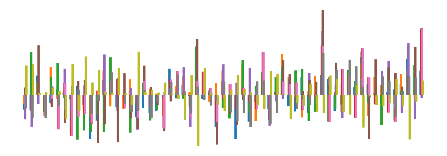
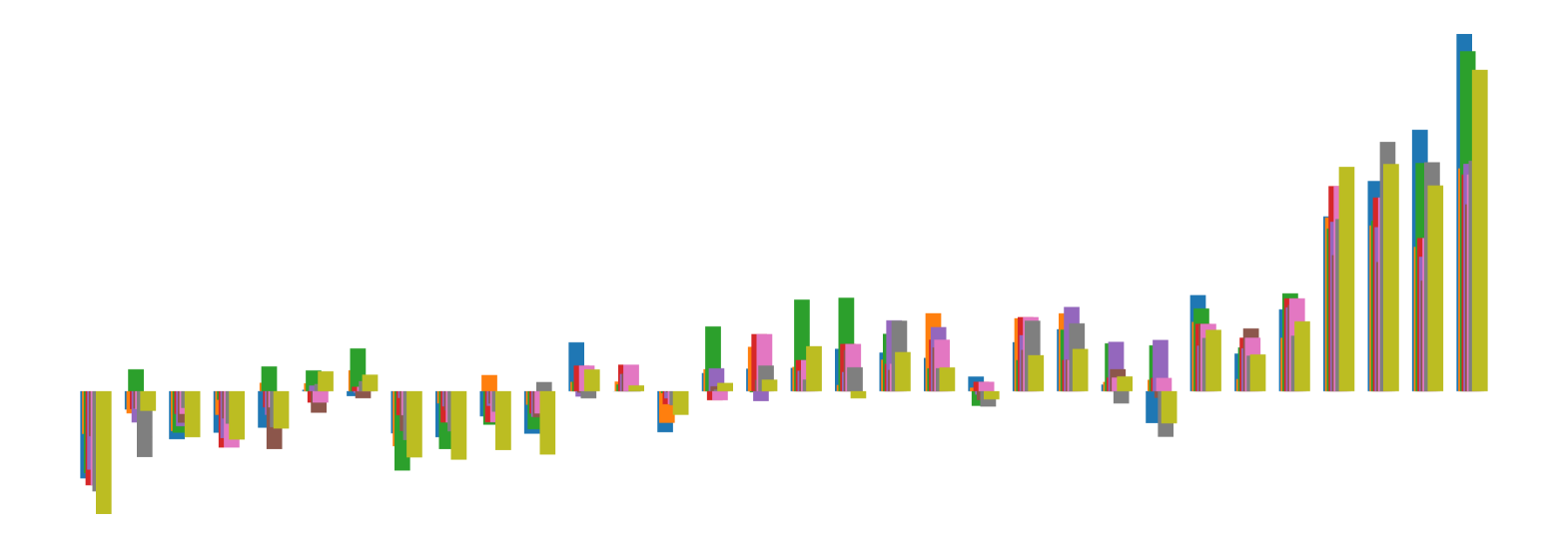
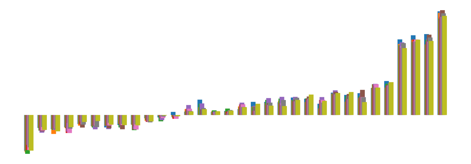
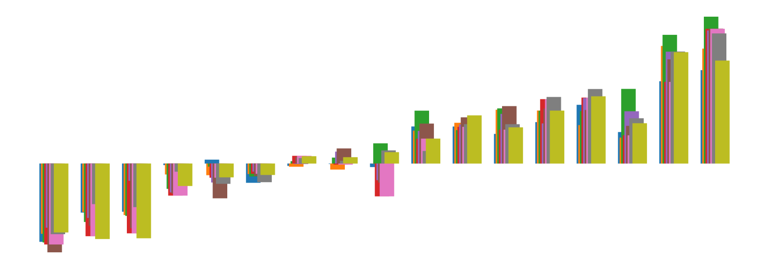
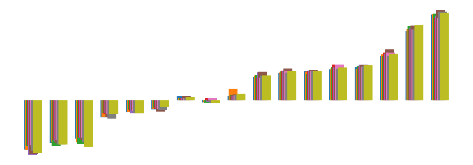
H.1 Attributions

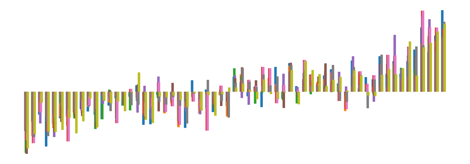
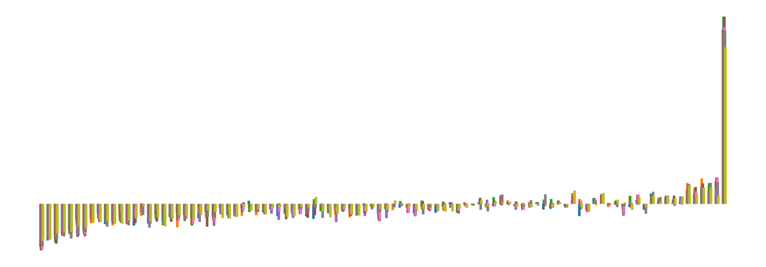
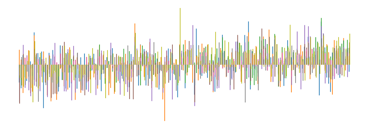
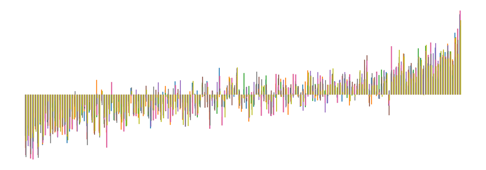
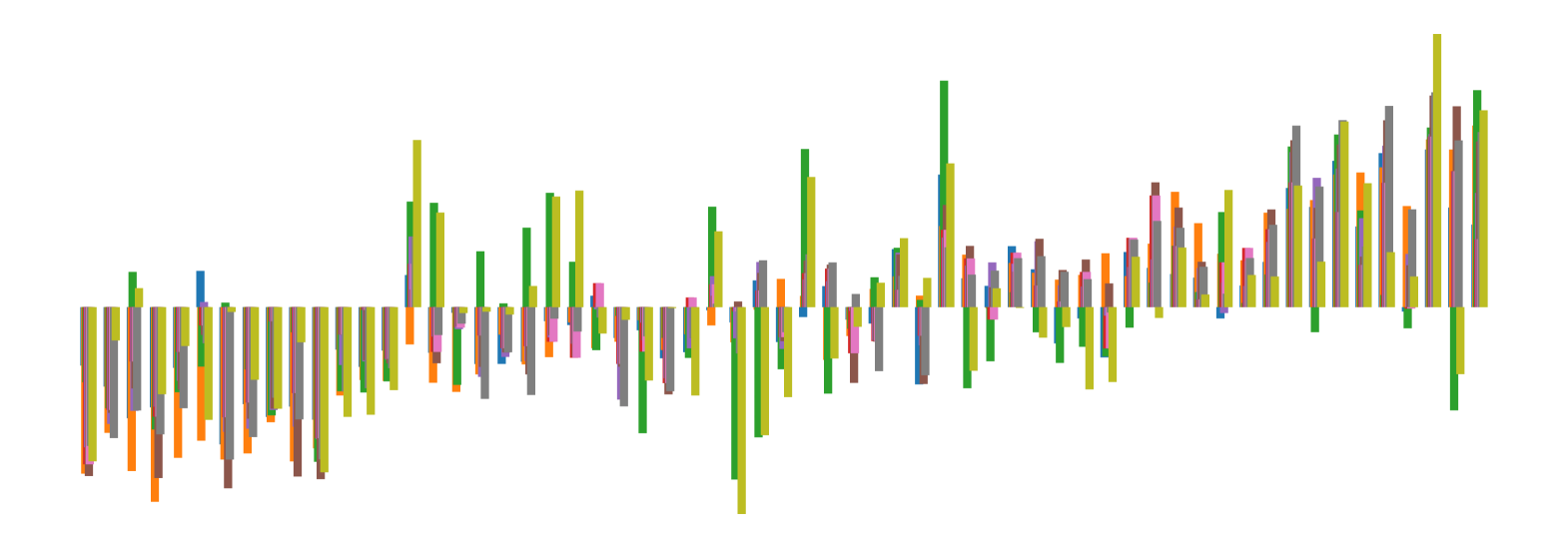
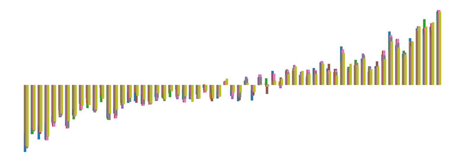
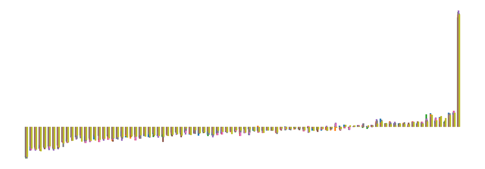
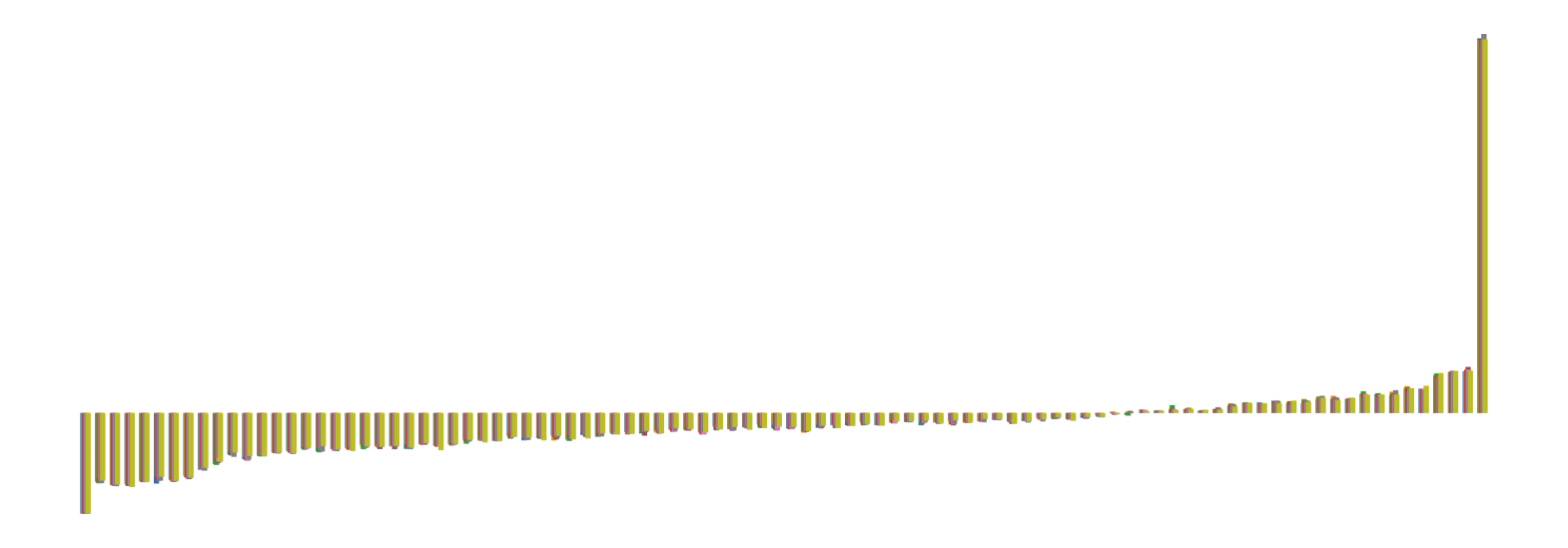
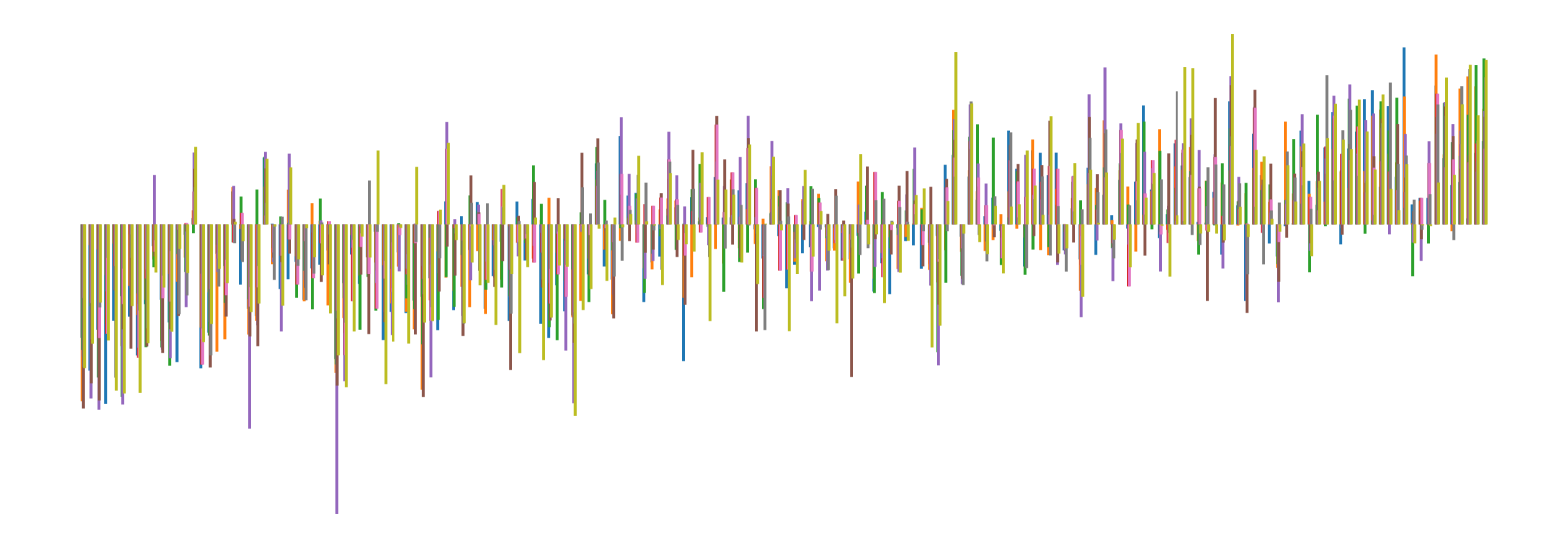
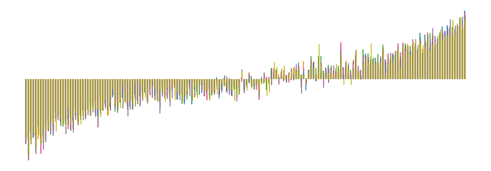
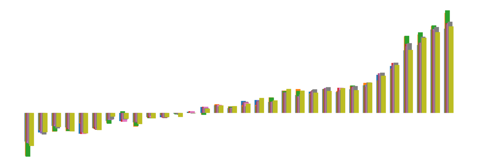
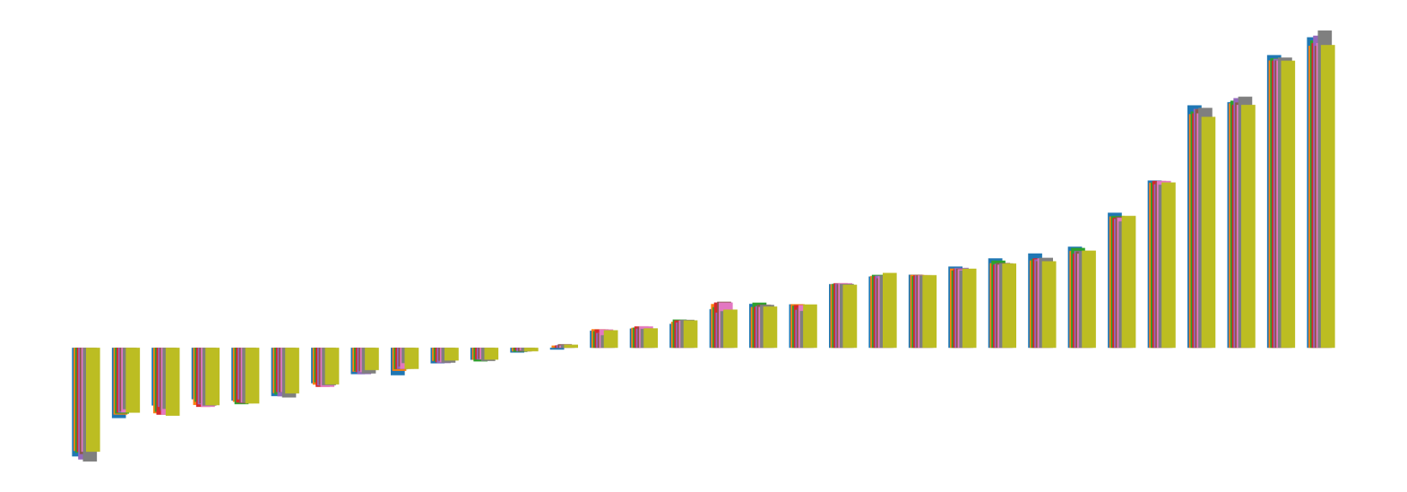
We pictorially show the inconsistency of individual model feature attributions versus the consistency of attributions ensembles of 15 for each tabular dataset in Figure 4 and Figure 5. The former shows inconsistency over differences in random initialization, the latter shows inconsistency over one-point changes to the training set.

H.2 Similarity Metrics of Attributions

We display how Spearman’s ranking coefficient ( $\rho$ ), Pearson’s Correlation Coefficient ( $r$ ), top-5 intersection and $\ell_{2}$ distance between feature attributions over the same point become more and more similar with increasing numbers of ensemble models. While the comparisons to generate the similarity score is between two models on the same point, the result is averaged over this comparison for the entire test set. We average this over 276 comparisons between different models. In cases were abstention is high, indicating inconsistency on the dataset for the training pipeline, selective ensembling can further improve stability of attributions by not considering unstable points (see e.g. German Credit). We present the expanded results from the main paper, for all datasets, on all four metrics (as SSIM is only computed for image datasets, and $\rho$ is not computed for image datasets). We display error bars indicating standard deviation over the 276 comparisons between two models for tabular datasets, and 40 comparisons for image datasets.

Selective Ensembling for Prediction Consistency

Appendix A Proofs

A.1 Proof of Theorem 3.1

Theorem 3.1.

Proof.

A.2 Proof of Theorem 4.1

Theorem 4.1.

Proof.

A.3 Proof of Corollary 4.2

Corollary 4.2.

Proof.

A.4 Proof of Corollary 4.3

Corollary 4.3.

Proof.

Appendix B Datasets

Appendix C Model Architecture and Hyper-Parameters

Appendix D Metrics

D.1 SSIM

Appendix E Experimental Results for α=0.01\alpha=0.01

Appendix F Selective Ensembling Full Results

Appendix G Selective Ensembles and Disparity in Selective Prediction

Appendix H Explanation Consistency Full Results

H.1 Attributions

H.2 Similarity Metrics of Attributions

Appendix E Experimental Results for $\alpha=0.01$