Selective Kalman Filter: When and How
to Fuse Multi-Sensor Information
to Overcome Degeneracy in SLAM
Abstract
Research trends in SLAM systems are now focusing more on multi-sensor fusion to handle challenging and degenerative environments. However, most existing multi-sensor fusion SLAM methods mainly use all of the data from a range of sensors, a strategy we refer to as the “all-in” method. This method, while merging the benefits of different sensors, also brings in their weaknesses, lowering the robustness and accuracy and leading to high computational demands. To address this, we propose a new fusion approach – Selective Kalman Filter – to carefully choose and fuse information from multiple sensors (using LiDAR and visual observations as examples in this paper). For deciding when to fuse data, we implement degeneracy detection in LiDAR SLAM, incorporating visual measurements only when LiDAR SLAM exhibits degeneracy. Regarding degeneracy detection, we propose an elegant yet straightforward approach to determine the degeneracy of LiDAR SLAM and to identify the specific degenerative direction. This method fully considers the coupled relationship between rotational and translational constraints. In terms of how to fuse data, we use visual measurements only to update the specific degenerative states. As a result, our proposed method improves upon the “all-in” method by greatly enhancing real-time performance due to less processing visual data, and it introduces fewer errors from visual measurements. Experiments demonstrate that our method for degeneracy detection and fusion, in addressing degeneracy issues, exhibits higher precision and robustness compared to other state-of-the-art methods, and offers enhanced real-time performance relative to the “all-in” method. The code is openly available.
Index Terms:
Kalman filter, multi-sensor fusion, degeneracy, LIO, VIO, SLAM.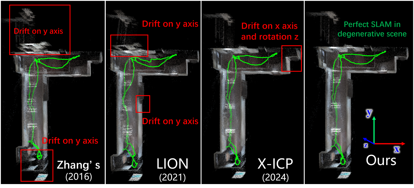
I INTRODUCTION
Simultaneous localization and mapping (SLAM) plays a significant role in robotics, autonomous driving, and Augmented Reality. To address challenging environments and to enhance localization robustness and environmental perception, there is an increasing focus on SLAM systems that fuse multiple sensors [1]. These systems typically integrate a combination of sensors such as LiDAR, vision, RGB-D camera, and IMU, exemplified by R3LIVE [2], FAST-LIVO [3], LVIO-Fusion [4], RIVER [5], etc.
Existing Kalman filter research [6, 7] has focused on multi-sensor information fusion, which propose using an Extended Kalman Filter (EKF) and an adaptive fuzzy logic system to fuse odometry and sonar signals. The core idea of these studies are to adaptively adjust the gain. Sun et al. [8] present a new multi-sensor optimal information fusion criterion weighted by matrices within the framework of linear minimum variance. By determining the cross-covariance, they then establish the optimal fusion matrix weights. To address the issue of occasional GPS signal loss or inaccuracies, Farhad [9] applies the KF to incorporate GPS measurements into the data fusion process, utilizing GPS data heavily only when it becomes reliably available. However, these works primarily focus on how to utilize and merge information from multiple sensors, without considering the necessity of fusion or integrating all available data. When fusing high-precision data with moderate-precision data in non-degenerative conditions, the accuracy improvement is often minimal or even negative, and it also incurs additional computational costs. We refer to this indiscriminate fusion of all measurement data as the “all-in” method. This approach faces two main issues:
First, the “all-in” method, by processing a volume of information than single-sensor SLAM, often results in significant computational burden, impacting real-time performance.
Second, while integrating the advantages of various sensors, the “all-in” method also incorporates their disadvantages. For instance, visual SLAM is frequently affected by motion blur, drastic lighting changes, and dynamic objects, leading to substantial errors or even system failure.
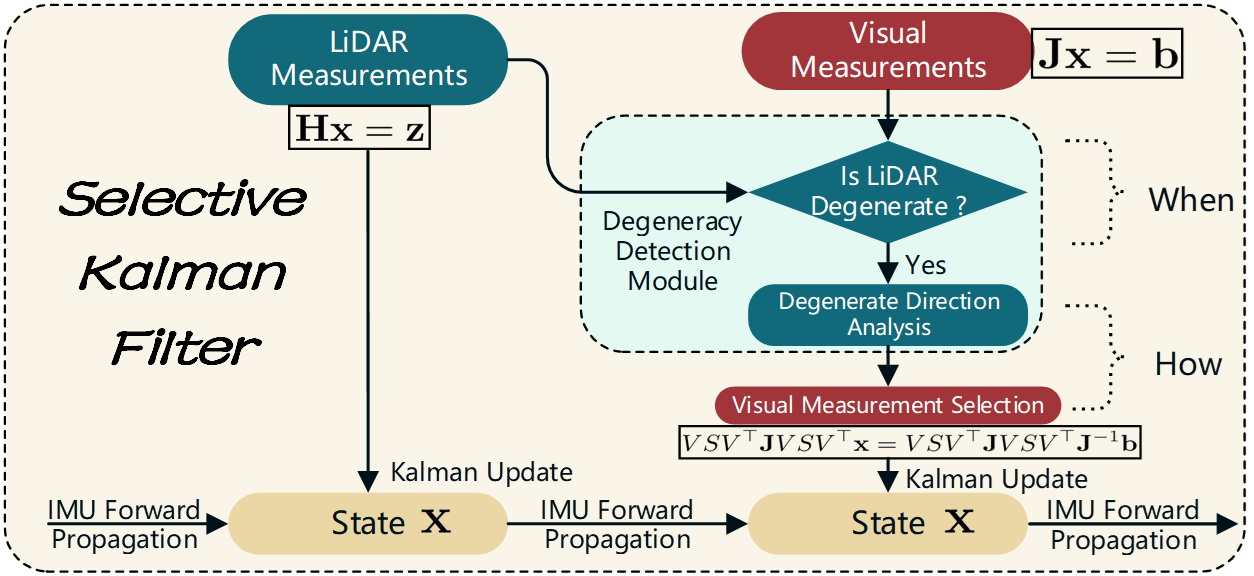
Accordingly, this paper addresses the two aforementioned issues by discussing when and how to selectively fuse multi-sensor information, using a LiDAR and vision-integrated SLAM system as an example. A critical consideration in multi-sensor fusion for SLAM is that individual sensors are prone to localization degeneracy, whereas incorporating different sensor types can provide additional constraints and prevent SLAM degeneracy.
For the “when” aspect, our solution is to integrate visual information only when the more accurate and robust LiDAR SLAM subsystem shows signs of degeneracy, relying solely on the LiDAR subsystem for pose estimation otherwise.
Regarding “how” to fuse, if all information is merged, the lower precision of the visual subsystem might reduce the overall accuracy of the LiDAR system. Therefore, our solution is to fuse visual information only in the directions where the LiDAR subsystem is degenerative.
The solution to “when” requires accurately determining whether degeneracy has occurred in LiDAR SLAM. Existing research in this area includes Zhang’s work [10], which assesses degeneracy by evaluating the condition number of the approximate Hessian matrix. However, due to the differing units and magnitudes of rotation and translation within the state, the eigenvalues of the approximate Hessian matrix couple rotation and translation. Consequently, the derived condition number is not dimensionless, making it challenging to accurately assess degeneracy in practical applications. Similarly, Hinduja’s approach [11] relies on comparing eigenvalues with thresholds for degeneracy detection, but this method also suffers from the issue of non-uniform dimensions in eigenvalues, complicating the establishment of fixed thresholds. To tackle these challenges, LION [12] and Switch-SLAM [13] introduce strategies that leverage submatrices of the Hessian matrix for independent degeneracy assessment in rotation and translation. The uniform dimensions within each submatrix endow the eigenvalues with a clear geometric significance, facilitating the application of fixed thresholds for degeneracy analysis. Based on this approach, X-ICP [14] also applies normalization and removes mostly noisy data with little contribution. However, these approaches do not account for the high degree of coupling between rotation and translation in point-plane constraints, leading to inaccuracies in determining the extent and direction of degeneracy. MM-LINS [15] is our previously proposed work, which includes degeneracy detection, but it does not have a dedicated analysis and experiments specifically for degeneracy detection. Julian [16] proposed a learning-based method for degeneracy detection. However, this approach is notably time-consuming and relies solely on current point clouds, which are insufficient for comprehensive degeneracy assessment without incorporating historical point cloud data. Moreover, this method suffers from a lack of generalizability.
Our proposed solution to “how” entails accurately determining the direction of degeneracy in LiDAR SLAM, incorporating visual measurements exclusively in these degenerative directions. Conversely, the fusion approach by LION [12] ceases the use of LiDAR odometry upon any LiDAR degeneracy, switching instead to other odometries. This method is somewhat rudimentary, as relying on lower accuracy and robustness sensor information in non-degenerative directions can actually diminish system performance. The methodologies of Zhang [10], Hinduja [11], and X-ICP [14] advocate for fusing information from other sensors only in degenerative directions, a strategy we consider to be optimal. However, these methods, which are optimization-based, do not address a filtering-based framework, nor can they precisely identify the specific directions of degeneracy. This can result in the true degenerative directions not being adequately constrained following by other sensor measurements.
Therefore, this paper introduces the Selective Kalman Filter to concretely implement the “when” and “how” solutions in selective data fusion. “Selective” here refers to the careful selection of the appropriate timing and data for fusion. We employ the advanced vision-LiDAR fusion scheme R3LIVE as a baseline for deploying the Selective Kalman Filter algorithm. The comparative results of the experiment are shown in Fig. 1. The specific contributions of this paper are:
-
•
We introduce a novel multi-sensor fusion approach, named the Selective Kalman Filter, designed to address when and how to selectively fuse data. This method integrates necessary visual information only when LiDAR data is degenerate, significantly enhancing real-time performance while ensuring robustness and accuracy.
-
•
We introduce an innovative and efficient method for degeneracy detection in LiDAR odometry, which also enables the determination of the degenerative direction. This approach fully considers the coupled relationship between rotational and translational constraints.
-
•
Through experiments, we demonstrate the accuracy of the proposed degeneration detection method and the efficiency of the Selective Kalman Filter.
-
•
We open-source the code for broader accessibility and community engagement.
II NOTATION
In this study, we simply define the state
| (1) |
where and represent rotation and translation, respectively. Within the framework of Kalman Filter, we define the measurement equation for point-to-plane constraints derived from LiDAR [17], following its linearization, as
| (2) |
where is the Jacobin matrix of dimensions , with representing the number of point-to-plane measurements. is the measurement vector, and comes from the raw LiDAR measurements.
Similarly, the linearized measurement equation for visual data is
| (3) |
where is the Jacobin matrix of dimensions , and denotes the number of visual measurements. is the measurement vector, and comes from the raw visual measurements. In the following sections, we adopt the convention of using uppercase letters to denote matrices and lowercase letters for vectors.
III SYSTEM OVERVIEW
First, we introduce the “all-in” method for LiDAR-inertial-vusial SLAM, as exemplified in methodologies like FAST-LIVO [3], R3LIVE [2]. In the absence of visual or LiDAR measurements, similar to FAST-LIO2 [18], the system uses the IMU’s acceleration and angular velocity for integration to propagate the state, serving as the prediction step in Kalman Filter. When LiDAR or visual measurements come, the system proceeds with data fusion updates in the Kalman Filter.
To the best of our knowledge, under conditions where neither system degenerates, LiDAR-inertial odometry (LIO) systems demonstrate higher accuracy and greater robustness compared to visual-inertial odometry (VIO) SLAM [19, 20]. In integrating the Selective Kalman Filter into the LiDAR-inertial-visual odometry (LIVO) system, we prioritize the LIO subsystem as the core and the VIO subsystem as supplementary. The system’s workflow is illustrated in Fig. 2. Unlike the “all-in” method, our approach performs degeneracy detection and analysis based on LiDAR measurements:
If LIO subsystem is not degenerative, we opt not to fuse visual measurements. This approach helps prevent the introduction of errors caused by visual issues such as motion blur, overexposure, and incorrect feature matching. Additionally, it reduces computational load, thereby enhancing real-time performance.
If LIO subsystem is degenerative, to minimally introduce visual information and prevent deterioration in state estimation, we analyze the LiDAR’s degenerative direction. We then selectively fuse visual data pertinent to this degenerative direction and discard data from non-degenerative directions, which helps prevent a decline in the accuracy of the LiDAR’s non-degenerative dimensions.
We refer to this method of selectively updating information fusion as the “Selective Kalman Filter”.
IV DEGENERACY DETECTION IN LIDAR SLAM
First, we transform the LiDAR measurement Equation (2) using a weighted linear least squares method, resulting in
| (4) |
where is the estimated value of state . For simplification, we have made the following definitions:
| (5) |
So Equation (5) can be simplified to
| (6) |
Due to noise in real-world scenarios, the matrix is invariably a full rank matrix. Consequently, it follows that is a real symmetric positive-definite matrix.
Hinduja’s method [11] for degenerative detection involves comparing the smallest eigenvalue of with a predefined threshold. However, it is important to note that, since the first three dimensions of represent rotation and the last three represent translation, the eigenvalues obtained from the eigenvalue decomposition of the matrix represent values coupled with both rotation and translation. These values lack a clear physical meaning, as their units are related to both rotation and translation. Furthermore, even within the same eigenvalue decomposition of , the eigenvalues have different units. Therefore, it becomes challenging to set a reasonable threshold for degeneracy detection. Moreover, the eigenvectors corresponding to these eigenvalues do not represent any actual directions in the real world. Consequently, this method is often impractical for deployment.
To address this issue, LION [12] proposes that degeneracy and its direction can be determined by analyzing the diagonal elements of the . Let us first express the matrix in the form of a block matrix
| (7) |
LION separately performs eigenvalue decomposition on the and :
| (11) | |||||||
| (15) |
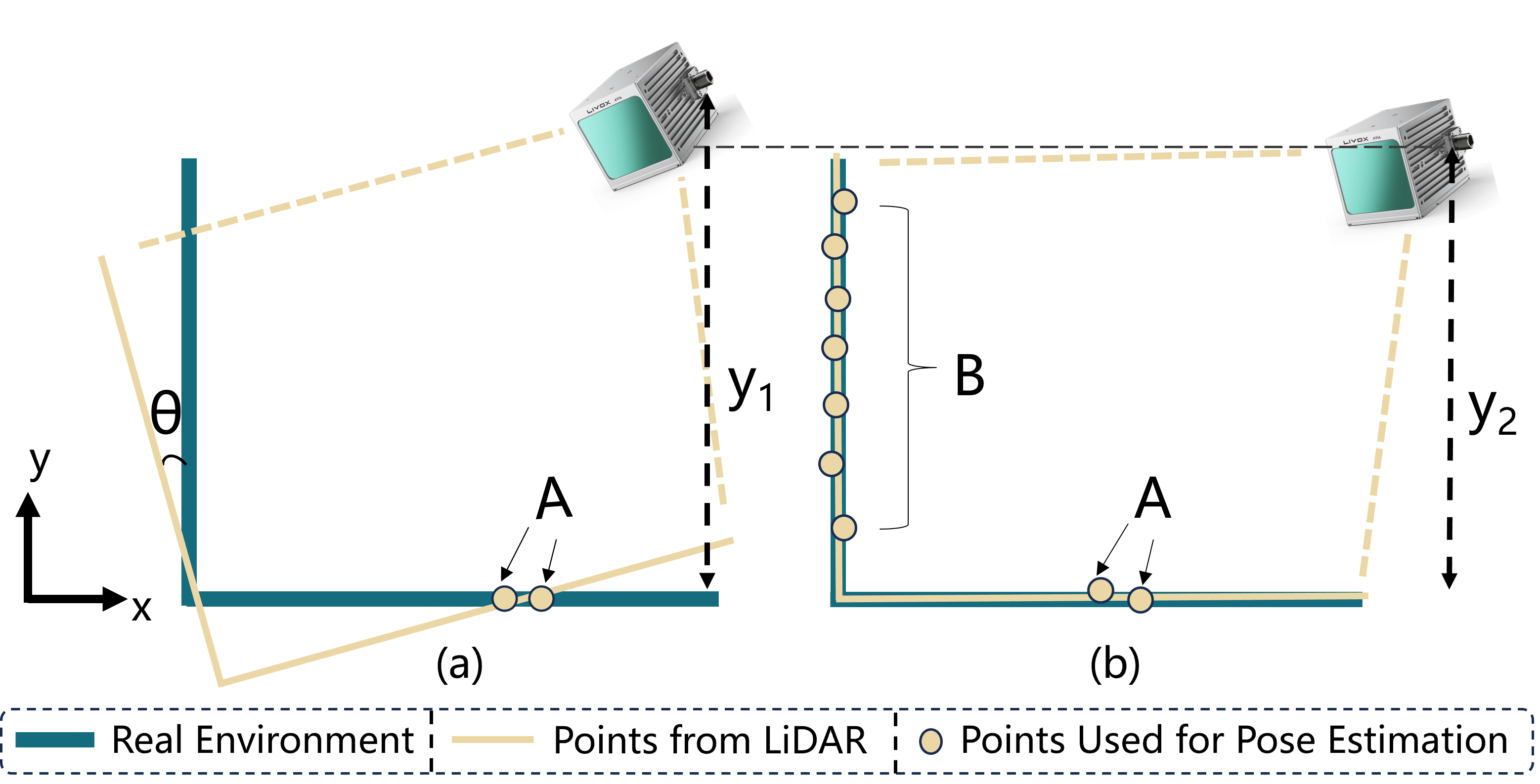
It then sets two thresholds to assess whether there is degeneration in rotation and translation. It’s worth mentioning that this method effectively resolves the issue in Hinduja’s approach where threshold values lack physical significance and cannot be fixed. However, by overlooking the coupled terms and , it neglects the mutual influence between rotational and translational constraints. Consequently, the degenerative level and direction estimated by this method are often inaccurate in most scenarios. As illustrated in Fig. 3 (a), according to LION’s perspective, the estimation in the -direction is solely dependent on the Jacobians of point-plane residuals in the -direction involving points A, leading to poor estimation in the -direction, as shown by . However, in reality, point-plane residuals in the -direction involving points B can improve the estimation of rotation and consequently enhance the -estimation, as indicated by . It can be inferred that this latter approach, by considering translation and rotation in a coupled manner, provides higher accuracy for uncertain estimations.
To address the aforementioned issue, we propose a new, elegantly simple, and physically meaningful degeneracy detection method based on covariance information. Initially, we invert the matrix, thereby obtaining the covariance matrix for state :
| (16) |
It should be noted that
| (17) |
| (18) |
From Equation (17) and (18), it is apparent that our method is not equivalent to LION’s approach using a local Hessian matrix. Our method takes into account the coupled relationship between translation and rotation. It is evident from Equations (17) and (18) that our method takes into account the coupled relationship between rotation and translation. Additionally, this method has practical physical significance: the diagonal blocks of the covariance matrix represent the variances of the state, while the off-diagonal blocks indicate the correlations between different states. Variance serves as an intuitive measure of degeneracy level. For instance, a high variance indicates significant uncertainty in the estimation of that direction, signifying degeneracy.
We perform eigenvalue decomposition on and :
| (19) |
| (20) |
where the units for are squared angular units (, while the units for are squared length units ().
The columns in and corresponding to represent respective directions. At this point, both and are rotation matrices with practical physical significance, capable of rotating the original coordinate system to align with these characteristic directions. Consequently, we set two variance thresholds and based on practical requirements and experience. If , it indicates rotational degeneracy, with the corresponding eigenvectors representing the degenerative direction. The same principle applies to translation. It should noted that
| (21) |
which indicates that the principal directions derived from our covariance-based solution differ from those obtained through Hessian-based methods.
In summary, this section introduces a degeneracy detection method that has practical physical significance and takes into account coupled constraints. Theoretically, it is capable of more accurately determining the degree and degenerative direction.
V SELECTION OF VISUAL MEASUREMENTS
Initially, we apply a linear weighted least squares approach to the visual measurement Equation (3):
| (22) |
For simplification, we have made the following definitions:
| (23) |
So Equation (22) can be simplified to
| (24) |
Note that is always invertible according to the noise in the real world. Therefore, we obtain the estimated state
| (25) |
Using the eigenvector matrices of the covariance matrices and , we define a new rotation matrix, denoted as
| (26) |
It can rotate ’s coordinate system to align with the principal component directions of both translation and rotation:
| (27) |
Given the known dimensions corresponding to LiDAR subsystem, we define a selective matrix to select information in the visual measurement Equation (27) that aligns with the degenerative direction, thereby filtering out extraneous data:
| (28) |
For instance, if there is degeneracy in one translational and one rotational dimension within the LiDAR subsystem, such as when and , we set the selective matrix as
| (29) |
In this matrix, diagonal elements set to 1 correspond to degenerative state dimensions, while those set to 0 correspond to non-degenerative dimensions. We revert the state to its original coordinate system and simultaneously restore the original measurement equation:
| (30) |
To preserve the symmetry of the information matrix, we undertake further processing, resulting in
| (31) |
which can be implified to
| (32) |
where , .
At this point, we have completed the selection of visual data, retaining only the information pertinent to the direction of LiDAR degeneracy.
VI SELECTIVE KALMAN FILTER
First, we describe the conventional form of Kalman Filter. For the visual subsystem, it is assumed that there are pre-existing prior estimates, denoted as and covariance . Following the methodology used in FAST-LIO [17], the Kalman gain is calculated as
| (33) |
leading to the update equation
| (34) |
By substituting Equation (33) into the update Equation (34), we obtain
| (35) |
According to Equation (23), we can simplify Equation (35) to
| (36) |
where is posterior estimated state. Regarding the posterior covariance :
| (37) |
Substituting in (Equation (33)) and simplifying, we obtain
| (38) |
By observing the changes in the measurement equation for visual information before (Equation (24)) and after (Equation (32)), we can derive the new Selective Kalman Filter formula by simply replacing to and to :
| (39) |
| (40) |
Remark: In this paper, matrices subjected to eigenvalue decomposition are exclusively real symmetric matrices, thereby rendering the results of eigenvalue decomposition and singular value decomposition equivalent. Our primary goal is to identify the principal directions of these matrices, which essentially aligns with the physical implications associated with singular values. To streamline the presentation and reduce the number of variables, we uniformly describe the process using eigenvalue decomposition throughout the paper.
VII LIDAR-INERTIAL-VISUAL ODOMETRY
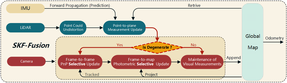
Building upon the excellent LIVO framework R3LIVE, we have integrated the Selective Kalman Filter, resulting in the creation of SKF-Fusion, as illustrated in Fig. 4. The original R3LIVE framework comprises two parallel subsystems: a direct method for LiDAR-Inertial Odometry (LIO) and a direct method for Visual-Inertial Odometry (VIO). Aspects identical to R3LIVE are not reiterated in this document. Based on this foundation, we conduct degeneracy assessments for the LIO subsystem. If no degeneration is detected, we solely utilize visual information for coloring, while concurrently preserving the map’s color information for use during degenerative states. In cases of degeneration, sequential updates between frames and between frames and the map are performed, focusing exclusively on the degenerative state components. In subsequent experiments, we evaluate SKF-Fusion using the R3LIVE dataset.
VIII EXPERIMENTS
Due to the limited availability of datasets containing LiDAR, vision, and IMU information compatible with R3LIVE, this study exclusively utilizes datasets [2, 21, 22] provided by R3LIVE for experimental analysis. The handheld device used to record the datasets includes a FLIR Blackfly BFS-u3-13y3c global shutter camera, Livox AVIA LiDAR, and an integrated IMU. Experiments were conducted on a computer equipped with an AMD 7840H CPU and running Ubuntu 20.04. We divided the experiments into two groups: degenerative datasets and normal datasets (the latter may also contain instances of weak degeneracy). For the degenerative datasets, we primarily assess the accuracy of our degeneracy detection method compared to other existing degeneracy detection methods, by measuring the impact on the precision and mapping quality of SKF-Fusion applied SLAM; for the non-degenerative datasets, we evaluate the improvements in accuracy and real-time performance of our SKF-Fusion compared to R3LIVE. The same configuration parameters, including voxel resolution and degeneracy threshold, were used throughout the experiments.
VIII-A Comparison in degenerative datasets
We conducted experiments on degenerative datasets in two outdoor scenes and one indoor scene, named degenerate_seq_00 to 02. We tested our method, X-ICP, LION, and Zhang’s method. If the moments of degeneracy are detected accurately, and the degenerative direction is precisely identified, we can successfully resist degeneracy by integrating visual information. We embedded these degeneracy detection methods within the SKF-Fusion framework, and to ensure a fair comparison, we used the same threshold for all experiments.
Remark: Since our method is based on the covariance matrix, while the LION, X-ICP, and Zhang’s methods are based on the information matrix, the covariance and information matrices are inversely related. Therefore, the thresholds for these methods should be reciprocal to each other. Specifically, for our method, degeneracy is considered when and . For the Hessian-based method, degeneracy is considered when and .
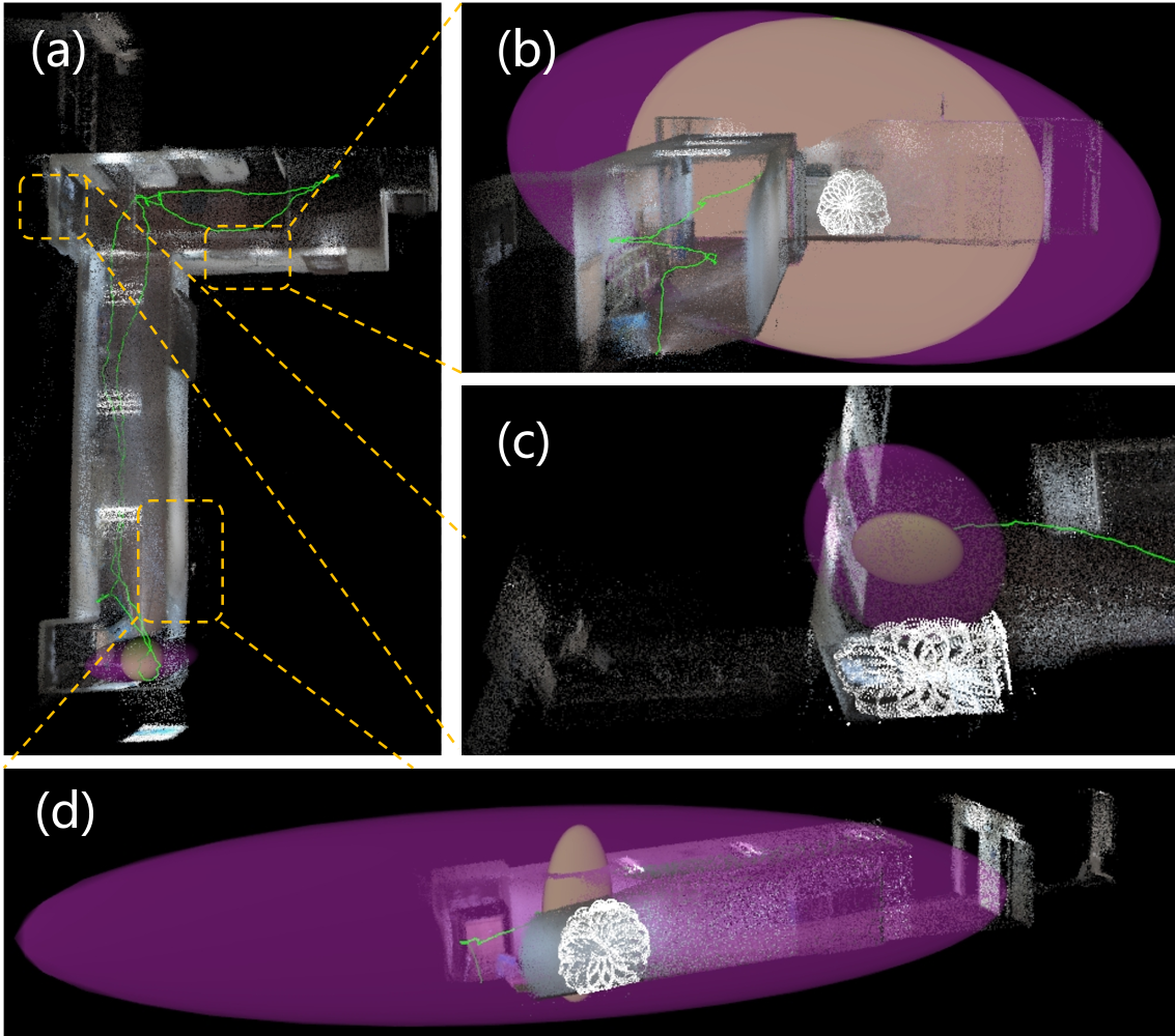
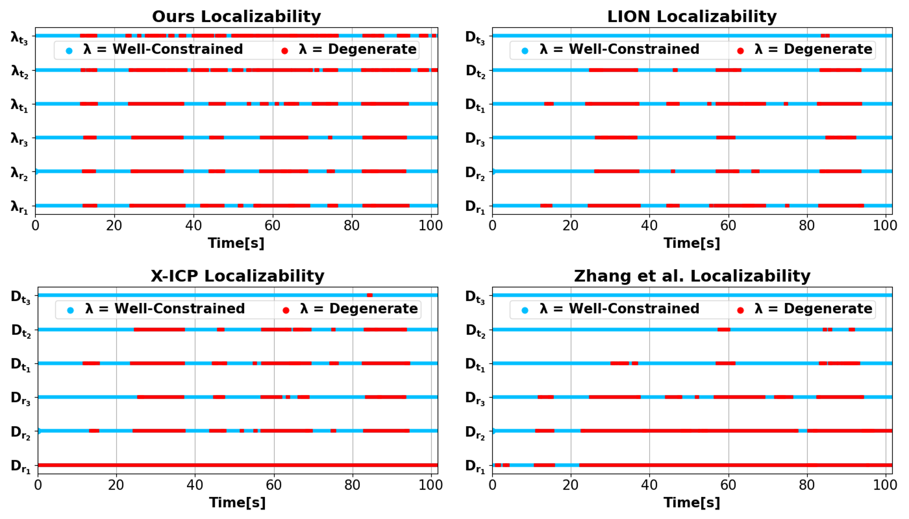
In the degenerate_seq_02 dataset, the LiDAR frequently faces a white wall, experiencing significant degeneracy, require visual observations for supplementation. The results of six-degree-of-freedom degeneracy detection using four different methods are illustrated in Fig. 6, with the localization and mapping outcomes shown in Fig. 1. From Fig. 1, it is evident that our method successfully resisted degeneracy, achieving high-precision localization and consistent mapping. In contrast, other methods, due to less accurate degeneracy detection, exhibited overlapping artifacts in mapping. In Fig. 6, compared to our method, LION appears overly optimistic, failing to detect degeneracy when it should. X-ICP, by filtering out many minor noise contributions, detected more instances of degeneracy than LION. However, due to a primary direction that differs from ours (indicated in Equation (21)), it still did not achieve optimal results. Zhang’s method significantly diverges from other degeneracy detection methods, mistakenly identifying moments of degeneracy as non-degeneracy and vice versa, indicating its relative ineffectiveness in practical degenracy detection tasks.
The translational uncertainty visualization of our covariance-based degeneracy detection method and the Hessian-based methods is shown in the Fig. 5. Corresponding to Equation (17) and (18), the Hessian-based methods are more optimistic than ours; hence, the brown ellipsoids are always inside the purple ellipsoids. Moreover, the principal directions of the brown ellipsoids do not align with those of the purple ellipsoids, and there are discrepancies in estimating the direction of greatest degeneracy, especially evident in Fig. 5(d): our method identifies the direction of greatest degeneracy as horizontal, whereas the Hessian-based methods consider it vertical, with the former being evidently more accurate.
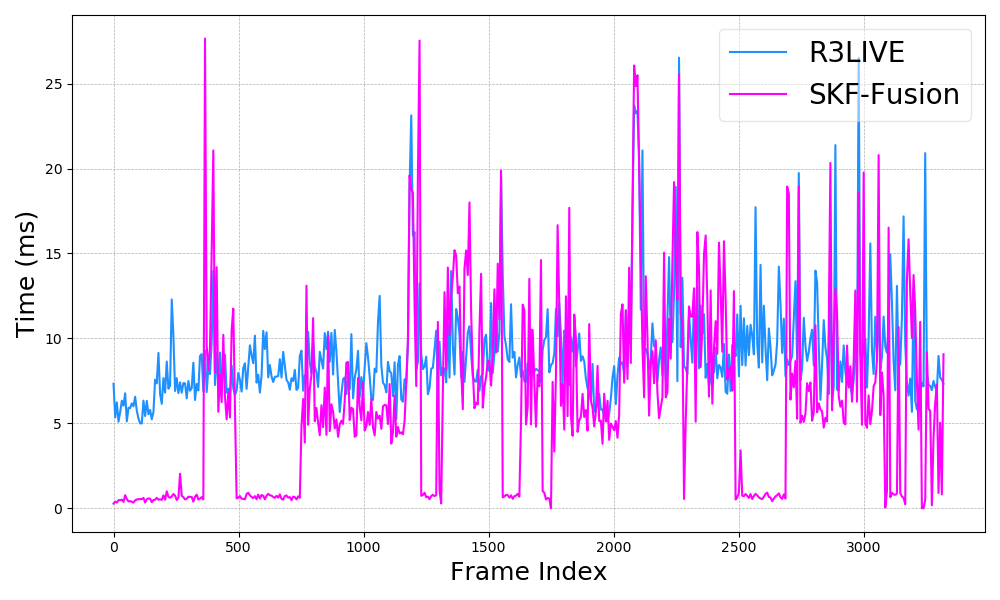
In this dataset, our method achieves accuracy comparable to R3LIVE (judged by end-to-end error and mapping results), but because SKF-Fusion only utilizes visual measurements for state updates during LiDAR degeneracy, the time cost of the visual subsystem is significantly reduced. When there is no degeneracy, only a minimal amount of time is spent on visual state maintenance, as shown in Fig. 7.
| degenerate_seq_00 | degenerate_seq_01 | degenerate_seq_02 | |
|---|---|---|---|
| R3LIVE | 0.067 | 0.094 | 0.100 |
| Zhang’s | 0.083 | 0.744 | 0.740 |
| LION | 0.072 | 5.781 | 0.116 |
| X-ICP | 0.082 | 1.214 | 1.827 |
| Ours | 0.061 | 0.109 | 0.097 |
-
1
The best results are in blod, while the second best are underlined.
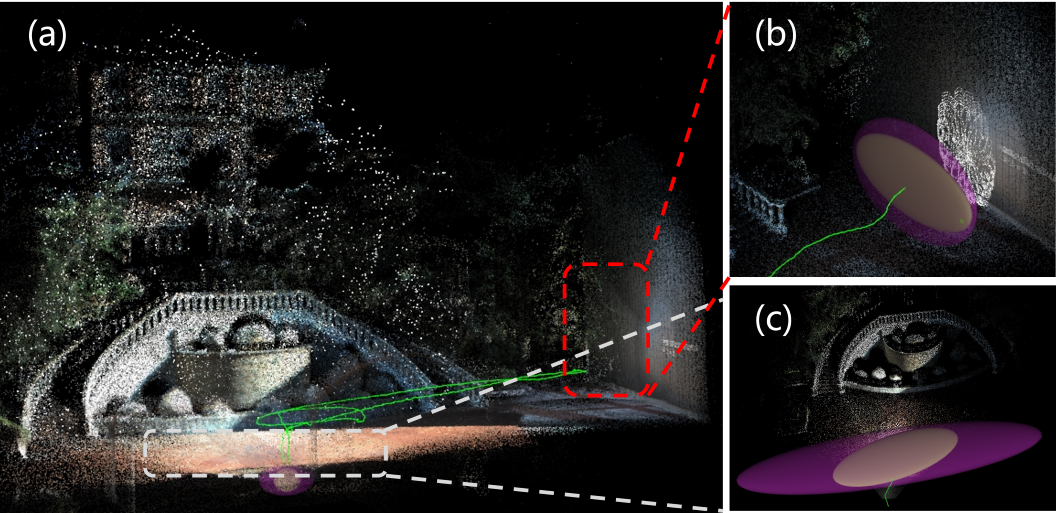
In the outdoor degenerate_seq_01 dataset, the LiDAR occasionally points towards the ground and walls, resulting in degeneracy across multiple degrees of freedom. The translational uncertainty is depicted as shown in the Fig. 8. We also implemented four different degeneracy detection methods in SKF-Fusion, with the SLAM outcomes presented as indicated in Fig. 9. It is evident that our method maintains high end-to-end accuracy and generates consistent maps without any ghosting effects.
In these three datasets, we evaluated the accuracy of R3LIVE and four degeneracy detection methods applied within SKF-Fusion. As shown in Table I, among the SKF-Fusion implementations utilizing the four degeneracy detection methods, the method we proposed achieved the best SLAM accuracy. This close resemblance in accuracy between our method and R3LIVE can be attributed to the datasets not introducing visual disturbances such as drastic lighting changes.

| SKF-Fusion | R3LIVE | |||
|---|---|---|---|---|
| ms | m | ms | m | |
| hku_main_building | 1.071 | 0.056 | 11.953 | 0.117 |
| hku_campus_seq_00 | 0.844 | 0.101 | 9.544 | 0.103 |
| hku_campus_seq_02 | 0.891 | 0.109 | 10.691 | 0.12 |
| hku_campus_seq_03 | 0.844 | 0.062 | 9.973 | 0.0701 |
| hku_park_00 | 0.797 | 0.08 | 13.113 | 0.076 |
| hku_park_01 | 0.861 | 0.553 | 11.744 | 0.61 |
VIII-B Comparison in normal datasets
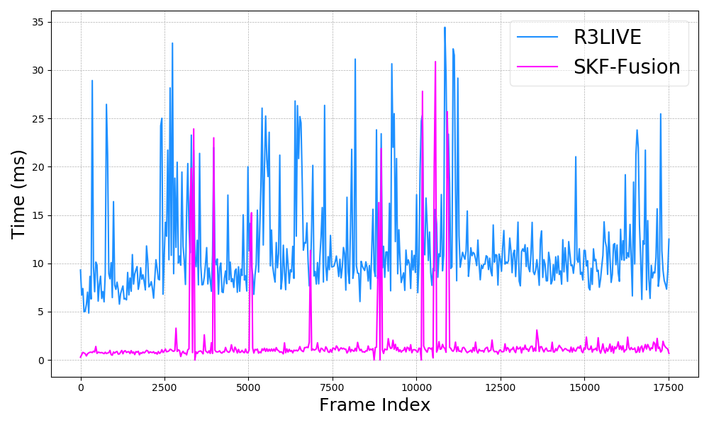
In normal datasets, significant degeneracy rarely occurs. Thus, these datasets are not effective for distinguishing between the performance of various degeneracy detection methods, nor do they significantly differentiate accuracy levels. However, they can be used to assess the real-time performance of R3LIVE compared to SKF-Fusion. As illustrated in Fig. 10, in the hku_main_building dataset (lasting approximately 1750 seconds), the time expenditure of the visual subsystem in SKF-Fusion is considerably less than that of R3LIVE, resulting in substantial computational resource savings. In most scenarios where LIO does not degenerate, the visual subsystem spends only 0-2 ms on visual information maintenance without performing state updates; under degenerative conditions, an additional 5-30 ms is required for integrating visual information with the radar subsystem to update the state. Time consumption and end-to-end error in other datasets are presented in Table II. From Table II, it can also be observed that due to predominantly relying on more accurate LiDAR measurements and less on visual measurements in most cases, there is a slight improvement in accuracy.
IX CONCLUSIONS
Building on the traditional foundation of “all-in” fusion SLAM involving LiDAR, vision, and IMU, this study introduces an innovative degeneracy detection module based on covariance information, along with a Selective Kalman Filter for the selective updating of degenerative states. Compared to other existing degeneracy detection methods, empirical evidence demonstrates that our proposed method significantly enhances the accuracy of degeneracy detection, thereby improving both the precision and robustness of localization. Notably, our approach substantially augments the real-time performance of the visual subsystem compared to the “all-in” method. It is important to mention that the current threshold selection does not robustly adapt to LIO across different voxel resolutions, highlighting an area for further research.
DISCUSSION AND FUTURE WORK
The Selective Kalman Filter extends beyond the fusion of LiDAR and vision, being applicable to a broad array of combinations, such as LiDAR with wheel encoders, Pedestrian Dead Reckoning (PDR), GPS, Ultra-Wideband (UWB), and more.
References
- [1] X. Xu, L. Zhang, J. Yang, C. Cao, W. Wang, Y. Ran, Z. Tan, and M. Luo, “A review of multi-sensor fusion slam systems based on 3d lidar,” Remote Sensing, vol. 14, no. 12, p. 2835, 2022.
- [2] J. Lin and F. Zhang, “R 3 live: A robust, real-time, rgb-colored, lidar-inertial-visual tightly-coupled state estimation and mapping package,” in 2022 International Conference on Robotics and Automation (ICRA). IEEE, 2022, pp. 10 672–10 678.
- [3] C. Zheng, Q. Zhu, W. Xu, X. Liu, Q. Guo, and F. Zhang, “Fast-livo: Fast and tightly-coupled sparse-direct lidar-inertial-visual odometry,” in 2022 IEEE/RSJ International Conference on Intelligent Robots and Systems (IROS). IEEE, 2022, pp. 4003–4009.
- [4] H. Zhang, L. Du, S. Bao, J. Yuan, and S. Ma, “Lvio-fusion:tightly-coupled lidar-visual-inertial odometry and mapping in degenerate environments,” IEEE Robotics and Automation Letters, vol. 9, no. 4, pp. 3783–3790, 2024.
- [5] T. Wen, Y. Fang, B. Lu, X. Zhang, and C. Tang, “Liver: A tightly coupled lidar-inertial-visual state estimator with high robustness for underground environments,” IEEE Robotics and Automation Letters, vol. 9, no. 3, pp. 2399–2406, 2024.
- [6] J. Sasiadek and P. Hartana, “Sensor data fusion using kalman filter,” in Proceedings of the Third International Conference on Information Fusion, vol. 2. IEEE, 2000, pp. WED5–19.
- [7] G. Rigatos and S. Tzafestas, “Extended kalman filtering for fuzzy modelling and multi-sensor fusion,” Mathematical and computer modelling of dynamical systems, vol. 13, no. 3, pp. 251–266, 2007.
- [8] S.-L. Sun and Z.-L. Deng, “Multi-sensor optimal information fusion kalman filter,” Automatica, vol. 40, no. 6, pp. 1017–1023, 2004.
- [9] F. Aghili and A. Salerno, “Driftless 3-d attitude determination and positioning of mobile robots by integration of imu with two rtk gpss,” IEEE/ASME Transactions on Mechatronics, vol. 18, no. 1, pp. 21–31, 2011.
- [10] J. Zhang, M. Kaess, and S. Singh, “On degeneracy of optimization-based state estimation problems,” in 2016 IEEE International Conference on Robotics and Automation (ICRA). IEEE, 2016, pp. 809–816.
- [11] A. Hinduja, B.-J. Ho, and M. Kaess, “Degeneracy-aware factors with applications to underwater slam,” in 2019 IEEE/RSJ International Conference on Intelligent Robots and Systems (IROS), 2019, pp. 1293–1299.
- [12] A. Tagliabue, J. Tordesillas, X. Cai, A. Santamaria-Navarro, J. P. How, L. Carlone, and A.-a. Agha-mohammadi, “Lion: Lidar-inertial observability-aware navigator for vision-denied environments,” in Experimental Robotics: The 17th International Symposium. Springer, 2021, pp. 380–390.
- [13] J. Lee, R. Komatsu, M. Shinozaki, T. Kitajima, H. Asama, Q. An, and A. Yamashita, “Switch-slam: Switching-based lidar-inertial-visual slam for degenerate environments,” IEEE Robotics and Automation Letters, vol. 9, no. 8, pp. 7270–7277, 2024.
- [14] T. Tuna, J. Nubert, Y. Nava, S. Khattak, and M. Hutter, “X-icp: Localizability-aware lidar registration for robust localization in extreme environments,” IEEE Transactions on Robotics, vol. 40, pp. 452–471, 2024.
- [15] Y. Ma, J. Xu, S. Yuan, T. Zhi, W. Yu, J. Zhou, and L. Xie, “Mm-lins: a multi-map lidar-inertial system for over-degenerate environments,” IEEE Transactions on Intelligent Vehicles, pp. 1–11, 2024.
- [16] J. Nubert, E. Walther, S. Khattak, and M. Hutter, “Learning-based localizability estimation for robust lidar localization,” in 2022 IEEE/RSJ International Conference on Intelligent Robots and Systems (IROS), 2022, pp. 17–24.
- [17] W. Xu and F. Zhang, “Fast-lio: A fast, robust lidar-inertial odometry package by tightly-coupled iterated kalman filter,” IEEE Robotics and Automation Letters, vol. 6, no. 2, pp. 3317–3324, 2021.
- [18] W. Xu, Y. Cai, D. He, J. Lin, and F. Zhang, “Fast-lio2: Fast direct lidar-inertial odometry,” IEEE Transactions on Robotics, vol. 38, no. 4, pp. 2053–2073, 2022.
- [19] L. R. Agostinho, N. M. Ricardo, M. I. Pereira, A. Hiolle, and A. M. Pinto, “A practical survey on visual odometry for autonomous driving in challenging scenarios and conditions,” IEEE Access, vol. 10, pp. 72 182–72 205, 2022.
- [20] T.-M. Nguyen, M. Cao, S. Yuan, Y. Lyu, T. H. Nguyen, and L. Xie, “Viral-fusion: A visual-inertial-ranging-lidar sensor fusion approach,” IEEE Transactions on Robotics, vol. 38, no. 2, pp. 958–977, 2022.
- [21] Z. Lin, “R3LIVE Dataset,” https://github.com/ziv-lin/r3live_dataset, 2023, accessed: 2023-02-27.
- [22] J. Lin and F. Zhang, “R 3 live++: A robust, real-time, radiance reconstruction package with a tightly-coupled lidar-inertial-visual state estimator,” IEEE Transactions on Pattern Analysis and Machine Intelligence, pp. 1–18, 2024.