Self-consistent massive disks in triaxial dark matter halos

Our method, which is based closely on J2K, is as follows:

1. 1.

   Calculate the axisymmetric component of the potential and the elliptical perturbation in the potential induced by the triaxial halo (§ 2.2).

2. 2.

   Calculate the closed orbits and corresponding disk ellipticity for a given net perturbation to the potential (§§ 2.3 and 2.4).

3. 3.

   Calculate the elliptical perturbation in the potential induced by a given disk ellipticity (§ 2.5).

4. 4.

   Solve for the form of the net potential perturbation that satisfies all of the above constraints (§ 2.6).

Throughout this procedure, the halo is kept fixed, i.e. it does not respond to the presence of the disk. Therefore, the potential that should be used in the calculation is the real shape of the halo in which the disk lies, which is less triaxial than the shape the halo would have in the absence of baryonic processes (Kazantzidis et al., 2004; Bailin et al., 2005; Berentzen & Shlosman, 2006).

The main differences between this work and J2K are:

1. 1.

   Where J2K assumes a logarithmic potential for the halo, we evaluate the radial form of the potential directly from a density distribution motivated by cosmological simulations.

2. 2.

   Where J2K assumes a constant perturbation to the halo potential, we allow the perturbation to vary with radius and either evaluate it directly from a triaxial density distribution motivated by cosmological simulations or use parametrizations developed from measurements of halos in cosmological simulations.

3. 3.

   Where J2K assumes that the disk responds with a constant ellipticity, we allow the disk ellipticity to vary with radius.

Whenever we carry out numerical calculations in this paper, all radially-varying functions are tabulated on a radial grid sampled at $100$ radii $R_{i}$ spaced logarithmically between $0.1$ and $100$ kpc in order to finely sample the inner region of the disk where the quantities vary most rapidly; $50$ grid points lie at $R<1$ kpc. The functions are linearly interpolated between grid points when their values are required at arbitrary radii.

For the perturbative approach, we assume that within the plane of the disk (which we take to be $z=0$ for simplicity), the total potential can be written as

where $R$, $\theta$, and $z$ are the cylindrical coordinates. For the purposes of this paper, we will assume an elliptical perturbation (i.e., $m=2$) from now on (see Appendix A for a discussion of the $m=4$ mode). We assume that $f_{\mathrm{pert}}(R)$ is small and varies slowly with $R$. Note that for $f_{\mathrm{pert}}>0$, isopotentials are elongated along the $x$ axis and closed orbits in the disk are elongated along the $y$ axis.

Both the disk and halo contribute to both the axisymmetric and $m=2$ components of the potential:

To first order, the $m=2$ perturbation in the potential induces an $m=2$ perturbation in the surface density distribution of the otherwise exponential disk (see Appendix A for a justification of our decision to neglect the higher-order terms):

We assume ${\epsilon_{\mathrm{disk}}}(R)$, the ellipticity of the isodensity ellipse, is small and varies slowly with $R$. The axisymmetric component of the disk potential is given by

($y=R/2R_{d}$; see Freeman 1970; Binney & Tremaine 1987, eq. 2-168), where $I$ and $K$ are modified Bessel functions.

Given the density distribution of the dark matter halo, both axisymmetric and $m=2$ components of the halo potential can be evaluated. If the isodensity surfaces of the halo are self-similar ellipsoids, then the halo density can be written as:

where

For example, we can use an NFW form for the density:

(Navarro et al., 1996; Jing & Suto, 2002). We make no assumptions about the relative magnitudes of $a$, $b$, and $c$; they are simply the relative axis ratios along the $x$, $y$, and $z$ axes respectively. Therefore, the disk, which lies in the $xy$ plane, can be oriented in any of the principal planes of the halo.

We calculate the halo potential along the $x$ axis, $\Phi_{x}^{\mathrm{halo}}(R)\equiv\Phi^{\mathrm{halo}}(R,0,0)$, and along the $y$ axis, $\Phi_{y}^{\mathrm{halo}}(R)\equiv\Phi^{\mathrm{halo}}(0,R,0)$, by numerically integrating eq. (2-99) of Binney & Tremaine (1987) using $\rho(s)$ given in equation (8). This allows us to calculate $\Phi_{0}^{\mathrm{halo}}$ and $f_{\mathrm{pert}}^{\mathrm{halo}}$ as

and

In a triaxial potential, dissipative gas settles on stable closed loop orbits when such orbits exist (El-Zant, 2001). This is the case throughout the potential of a centrally-concentrated mass profile such as the NFW profile. Therefore, the structure of a galactic disk, which consists of gas clouds and stars formed within those gas clouds, is determined by the form of the closed orbits. These have been examined in detail by Schoenmakers et al. (1997), and simplified into a convenient form by HN06. These previous derivations have assumed that the perturbation to the potential is constant over the radial excursion of an orbit, which is not the case for the radially-varying perturbations that we wish to study. We have therefore rederived the equations for closed orbits within a radially-varying perturbation from the equations of motion. The orbits follow

with velocities

where $R_{0}$ and $\theta_{0}$ define the guiding center of the orbit, $\theta_{0}=\Omega_{0}\,t$, and the following functions of $\Phi_{0}(R)$ are evaluated at $R_{0}$:

The coefficients $a_{1m}$ and $a_{3m}$ quantify the degree to which the radius $R$ and angular velocity $V_{\theta}$ respectively, which are constant for a circular orbit, vary for a unit perturbation to the potential. Our expressions differ from those in HN06 for the following reasons: (1) we have taken the radial variation of the perturbation into account in our derivation of equation (19); (2) we have generalized the expression for $g_{m}(R)$ to be valid for all $m$, while the expression in HN06 is specific to $m=2$; (3) we have removed the factor of $f_{\mathrm{pert}}$ from the definitions of $a_{1m}$ and $a_{3m}$ for convenience later (note that these quantities still depend implicitly on $f_{\mathrm{pert}}$ through its derivative); and (4) we have generalized the expression for $a_{3m}$ to be valid for all potential profiles, while the expression in HN06 is only valid when $g_{2}(R)=-3$, which is not the case in the inner regions of an NFW potential.

Given the tabulated values of $\Phi_{0}$, these functions can be evaluated at the grid points $R_{i}$. Because $\Phi_{0}$ has been calculated from analytic functions, the tabulated values are relatively free of noise and even the numerical second derivative does not contain large fluctuations. Note that the closed orbits are elongated perpendicular to the isopotential contours.

The disk must satisfy the continuity equation. In cylindrical coordinates:

We substitute $\Sigma(R,\theta)$ from (4), $V_{R}(R,\theta)$ from (13), and $V_{\theta}(R,\theta)$ from (14). To first order in the small quantities $f_{\mathrm{pert}}$, $\epsilon_{\mathrm{disk}}$, and their derivatives:

The neglected second-order terms induce small $m=4$ perturbations in the disk; see Appendix A for details.¹¹1We have also omitted the term in equation (22) that is proportional to $R\>\mathrm{d}(f_{\mathrm{pert}}\,a_{12})/\mathrm{d}R$; however, its effect is negligible. Equation (22) provides us with a relationship between the radial profile of the potential (embodied in $a_{12}$, $a_{32}$ and $V_{c}$), the strength of the perturbation in the net potential ($f_{\mathrm{pert}}$), and the ellipticity of the disk ($\epsilon_{\mathrm{disk}}$).

The ellipticity of the disk generates an $m=2$ perturbation to the disk potential. We calculate this as follows:

(Binney & Tremaine, 1987, eq. 2P-8). We restrict ourselves to the plane $z=0$, corresponding to an infinitely thin disk.

For small perturbations, the perturbed surface density is

Substituting (24) into (23), we note that the integral over $\mathrm{d}\theta^{\prime}$ vanishes except when $m=\pm 2$. Since $\int_{0}^{2\pi}\cos 2\theta^{\prime}\,e^{\pm i2\theta^{\prime}}\,\mathrm{d}\theta^{\prime}=\pi$, $e^{ix}+e^{-ix}=2\cos x$, and $J_{2}(x)=J_{-2}(x)$, we find

We can express $(R^{\prime}/R_{d})\,{\epsilon_{\mathrm{disk}}}(R^{\prime})$ in the final integral in terms of $f_{\mathrm{pert}}$, $a_{12}$, $a_{32}$, and $V_{c}$ using (22):

Because we do not know a priori the net perturbation $f_{\mathrm{pert}}(R)$, we cannot immediately evaluate these integrals. However, if we can find a function $f_{\mathrm{pert}}^{\mathrm{proxy}}$ whose form is similar to $f_{\mathrm{pert}}$, i.e. if $f_{\mathrm{pert}}/f_{\mathrm{pert}}^{\mathrm{proxy}}$ is a slowly-varying function of $R$, then we can approximate the potential as:

Note that $a_{12}(R^{\prime})$ and $a_{32}(R^{\prime})$ depend implicitly on $f_{\mathrm{pert}}^{\mathrm{proxy}}(R^{\prime})$ through its derivative. A first approximation can be obtained by setting $f_{\mathrm{pert}}^{\mathrm{proxy}}=f_{\mathrm{pert}}^{\mathrm{halo}}$, whose values have been tabulated from (10). Because the integral over $R^{\prime}$ is independent of $R$ and the integral over $k$ is independent of $R^{\prime}$, the integrals can be evaluated independently on fine grids of $k$ and $R$, respectively. Using this technique, we calculate

at each grid point $R_{i}$. The perturbation potential due to the disk is then given by

Expressed in this form, the meaning of $\eta(R)$ becomes clear: it is the magnitude of the disk response to a unit perturbation in the potential.

For clarity, we repeat here the important equations:

(see eqs. 1 and 3), and

(repeated from eq. 29). The physical interpretation of these equations is that the disk response is proportional to the net perturbation $f_{\mathrm{pert}}$, which is itself the sum of the disk response and the imposed halo perturbation. The disk response is opposite in sign to the halo perturbation, so $f_{\mathrm{pert}}$ in the self-consistent solution must be reduced with respect to the imposed halo perturbation.

The self-consistent solution can be obtained by collection equations (30) through (33):

In other words, the response of the disk causes the overall potential perturbation to be reduced by a factor of $1+\eta(R)/\Phi_{0}(R)$. All terms on the right hand side have been tabulated at the grid points $R_{i}$, resulting in a trivial evaluation of $f_{\mathrm{pert}}(R)$.

Armed with this new estimate of $f_{\mathrm{pert}}$, we can reexamine equation (28), substitute $f_{\mathrm{pert}}^{\mathrm{proxy}}=f_{\mathrm{pert}}$, and calculate a new value of $\eta(R)$ and therefore of $f_{\mathrm{pert}}(R)$. We repeat this procedure until the maximum change between iterations in the quantity $f_{\mathrm{pert}}/f_{\mathrm{pert}}^{\mathrm{halo}}$, which is a robust indicator of the relative error in $f_{\mathrm{pert}}$, is less than $10^{-3}$ at all radii; this is typically achieved in $20$–$30$ iterations. We have confirmed for some specific cases that our solution agrees to within $\sim 2\%$ of the true solution (assumed to have converged after a very large number of iterations) at all radii, and to much higher precision at most radii (see Figure 1). Adopting a stricter convergence criterion has no effect on our results. The relatively large number of iterations is required in order to accurately capture the sharp feature where $f_{\mathrm{pert}}\rightarrow 0$ that is seen in the solutions (see § 3).

Given $f_{\mathrm{pert}}$, the disk ellipticity $\epsilon_{\mathrm{disk}}$ can be calculated as a function of radius directly from equation (22) and the forms of the closed orbits can be calculated from equations (11) – (14). This provides a complete description of the disk.

We demonstrate the main features of our models using a fiducial triaxial NFW halo with mass $M_{200}=10^{12}~{\mathrm{M}_{\sun}}$, axis ratios $b/a=0.8$ and $c/a=0.6$, and a concentration $c_{200}=12$.²²2$M_{200}$ and $c_{200}$ refer to the mass and concentration relative to the radius $r_{200}$, defined such that the mean density within $r_{200}$ is $200$ times the critical density. We assume the Hubble parameter $h=0.7$. These values are typical for galaxy-sized dark matter halos in cosmological simulations (Allgood et al., 2006). The disk rotation axis is aligned with the minor axis of the halo, in agreement with the orientation of the halo angular momentum in simulations (Bailin & Steinmetz, 2005). All disks have radial scalelengths $R_{d}=3.0~\mathrm{kpc}$, with masses that range from zero up to $10^{11}~{\mathrm{M}_{\sun}}$.

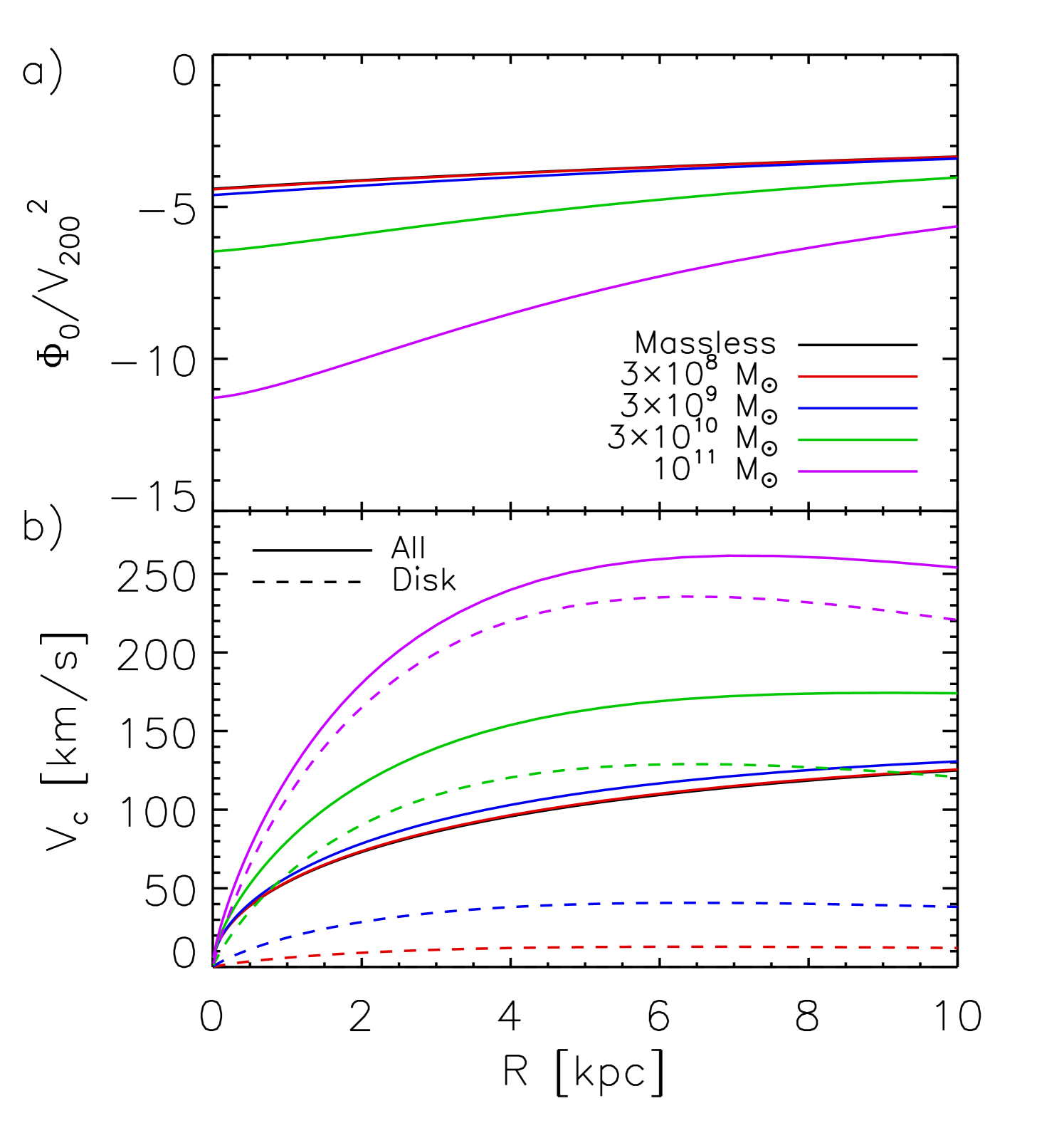
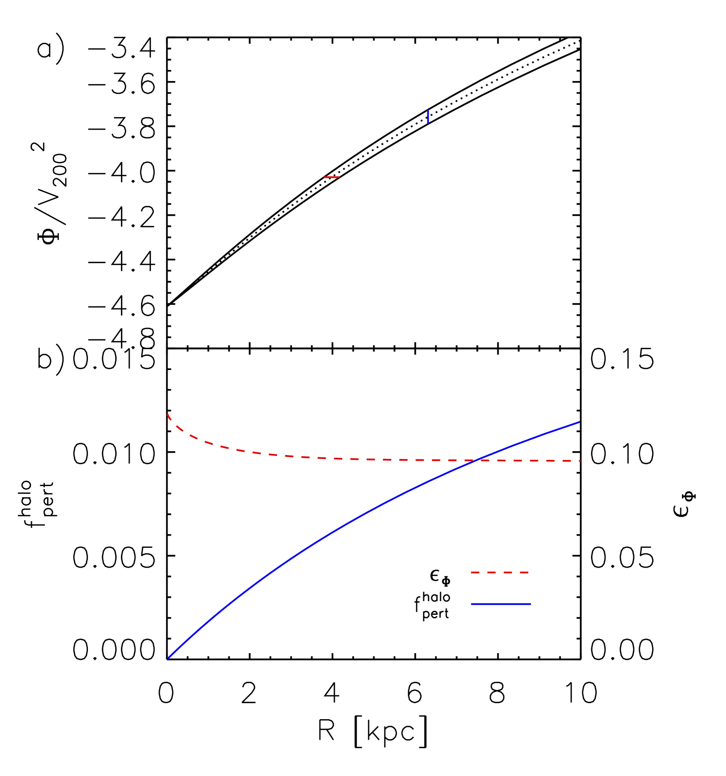
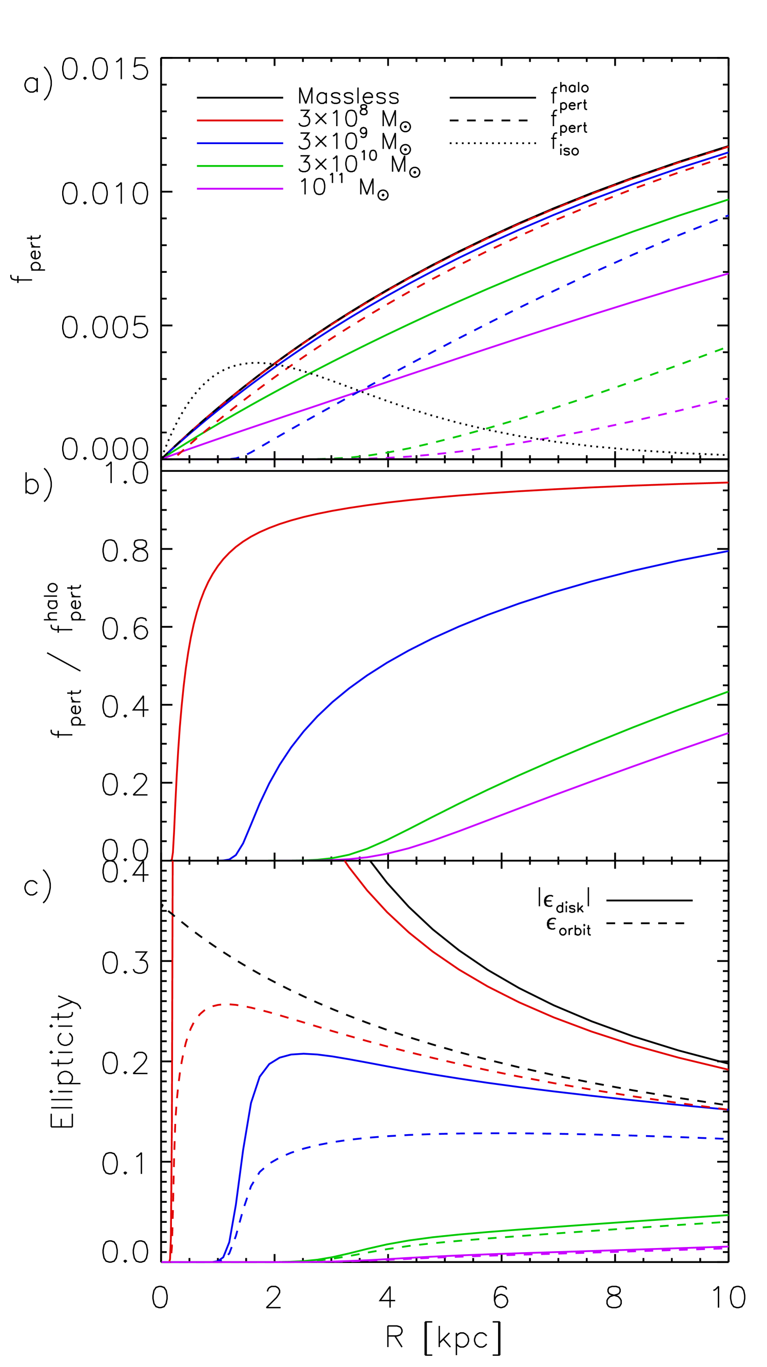
Figure 2 demonstrates how the axisymmetric component of the potential, $\Phi_{0}(R)$, and the rotation curve, $V_{c}(R)$, vary as a function of disk mass. The potential is given in units of $V_{200}^{2}\equiv G\,M_{200}/r_{200}$. For disk masses less then $3\times 10^{9}~{\mathrm{M}_{\sun}}$, the halo dominates the axisymmetric component of the potential at all radii, with the disk becoming increasingly more important with increasing disk mass beyond this. The non-axisymmetric component of the potential is demonstrated in Figure 3 for the $3\times 10^{9}~{\mathrm{M}_{\sun}}$ disk. Although the ellipticity of isopotential surfaces, $\epsilon_{\Phi}$, rises to small radii, the magnitude of the potential perturbation, $f_{\mathrm{pert}}^{\mathrm{halo}}$, must vanish at small radii because $\Phi_{x}(R=0)=\Phi_{y}(R=0)$ while $\Phi_{0}(R=0)$ reaches a finite value.

Figure 4a demonstrates both the initial halo perturbation ($f_{\mathrm{pert}}^{\mathrm{halo}}$, solid lines) and the net perturbation after including the self-consistent response of disk ($f_{\mathrm{pert}}$, dashed lines). Note that even though the halo is identical in each case, $f_{\mathrm{pert}}^{\mathrm{halo}}$ is lower for higher mass disks because the disk contributes to $\Phi_{0}$.

HN06 proposed that a suitable perturbation

(with $x\equiv R/r_{s}$, $a=0.1$, and $b=0.098$) would cause the rotation curve of a perturbed NFW profile to mimic that of a cored isothermal profile. We denote this as a dotted line in Figure 4a. The form of this perturbation is very different from the form of the perturbation that we find to be induced by a triaxial halo of uniform axis ratio, particularly once the self-consistent response of the disk is taken into account.

Figure 4b demonstrates the degree to which the initial halo perturbation $f_{\mathrm{pert}}^{\mathrm{halo}}$ is diluted by the self-consistent response of the disk. This is equal to $f_{\mathrm{pert}}/f_{\mathrm{pert}}^{\mathrm{halo}}$ and is determined from $1/(1+\eta(R)/\Phi_{0}(R))$. The ellipticity in the potential vanishes in the central region where $\eta(R)\gg\Phi_{0}(R)$. Even for a negligible disk mass, the potential in the innermost region is circularized. This region is larger for more realistic disks, which have a significant impact on the potential out to several disk scale lengths. As the disk mass increases, the form of the disk dominates both $\eta(R)$ and $\Phi_{0}(R)$, and therefore this function approaches an asymptotic form.

Comparison between Figure 4b and the equivalent figs. 2 and 3 of J2K reveals dramatically different behavior at small radii: in J2K, the “reduction factor” reaches a minimum at $1.42~R_{d}$ ($=4.26$ kpc for $R_{d}=3.0$ kpc) and then rises to unity, while in Figure 4b it falls monotonically to vanish at small radii. This is a direct result of the radial variation of $f_{\mathrm{pert}}$ in a physically realistic elliptical halo. Because $\eta(R)$ depends inversely on $f_{\mathrm{pert}}$ (see eq. 28), which must vanish at small radii, $\eta(R)$ must dominate over $\Phi_{0}(R)$ in the inner regions and the potential must become completely circularized.

In Figure 4c we plot the ellipticity of the disk isodensity contours (${\epsilon_{\mathrm{disk}}}$, solid lines) and of the orbits within the disk ($\epsilon_{\mathrm{orbit}}\equiv f_{\mathrm{pert}}\,a_{12}$, dashed lines). For a massless disk, we recover the results of HN06 that the ellipticity rises towards the center of the halo. However, the presence of a massive disk changes the situation dramatically. Because $f_{\mathrm{pert}}/f_{\mathrm{pert}}^{\mathrm{halo}}$ vanishes at small radii (Figure 4b), the equilibrium disk is axisymmetric at small radii. Even very low mass disks, which contribute negligibly to $\Phi_{0}$, still respond strongly enough to the elliptical potential to cause an important change in the behavior at small radii. We also note that the ellipticity of disk isophotes are always greater than ellipticity of orbits within the disk.

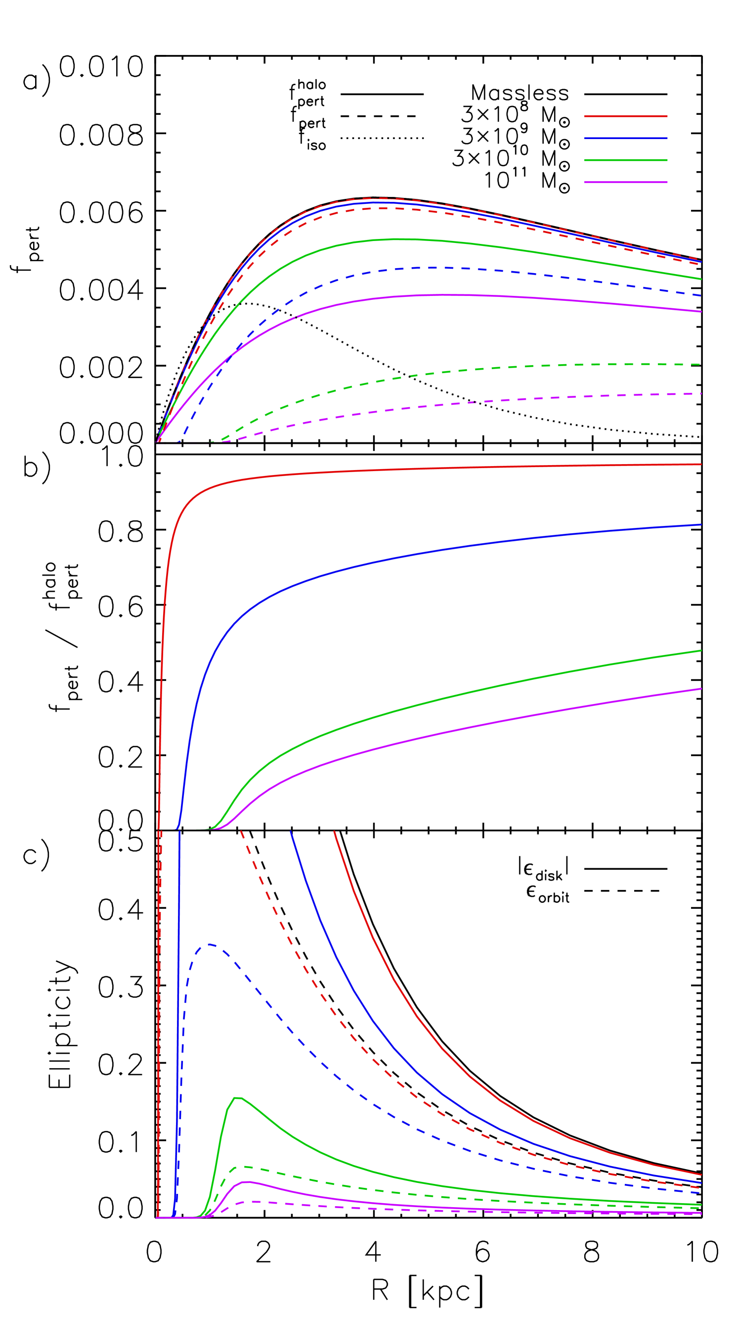
HNS found that the radial variation of the shape of the potential of cosmological $N$-body halos is not consistent with self-similar isodensity contours (see also Jing & Suto, 2002; Bailin & Steinmetz, 2005). They found instead that the isopotential axis ratios are well fit by the following function:

We have recomputed the self-consistent response of disks of varying mass in a potential of this form, with the values of the parameters taken from halo G4 of HNS, which has a very similar mass and concentration to the halo used in § 3.1. The results are shown in Figure 5. As noted by HNS, the perturbation in this case contains a peak at intermediate radius and is much more similar to the form of $f_{\mathrm{iso}}$ required by HN06 to fit LSB rotation curves, although unlike $f_{\mathrm{iso}}$ the perturbation remains more prominent to large radius. However, in many cases LSB rotation curves are only measured out to radii of a few kpc, so it is less clear what the required form of $f_{\mathrm{iso}}$ is at larger radii. The disks have less effect on the perturbation than in § 3.1; in particular, the radius inside which they circularize the potential is reduced, resulting in significantly more elliptical orbits at $1$–$3$ kpc than for the equivalent disks in a halo with constant axis ratios. Disk masses higher than $\sim 3\times 10^{9}~{\mathrm{M}_{\sun}}$ reduce the prominence of the peak in the perturbation and shift it to larger radii. The peak in $f_{\mathrm{pert}}^{\mathrm{halo}}$ could be moved to smaller radius, and therefore brought further into agreement with $f_{\mathrm{iso}}$, by reducing the $r_{\alpha}$ parameter in equation (36); however, this is unlikely to be a common situation, as G4 already has by far the lowest $r_{\alpha}$ value of any of the halos studied by HNS.

The effect of the baryonic disk on the shape of the halo is not yet well understood. Simulations suggest that halos containing baryonic disks are less elliptical than halos composed purely of dark matter, and that the circularization of the halo occurs most strongly at the center (Kazantzidis et al., 2004). If the intrinsic shape of the pure dark matter halo is well described by the HNS form, which is most elliptical at the center, baryonic processes may result in a situation more similar to the constant axis ratio case of § 3.1. We therefore expect that the regions in which these models differ most strongly, $1$–$3$ kpc, are also the regions where the unknown effect of disk formation introduces the most uncertainty into our models.

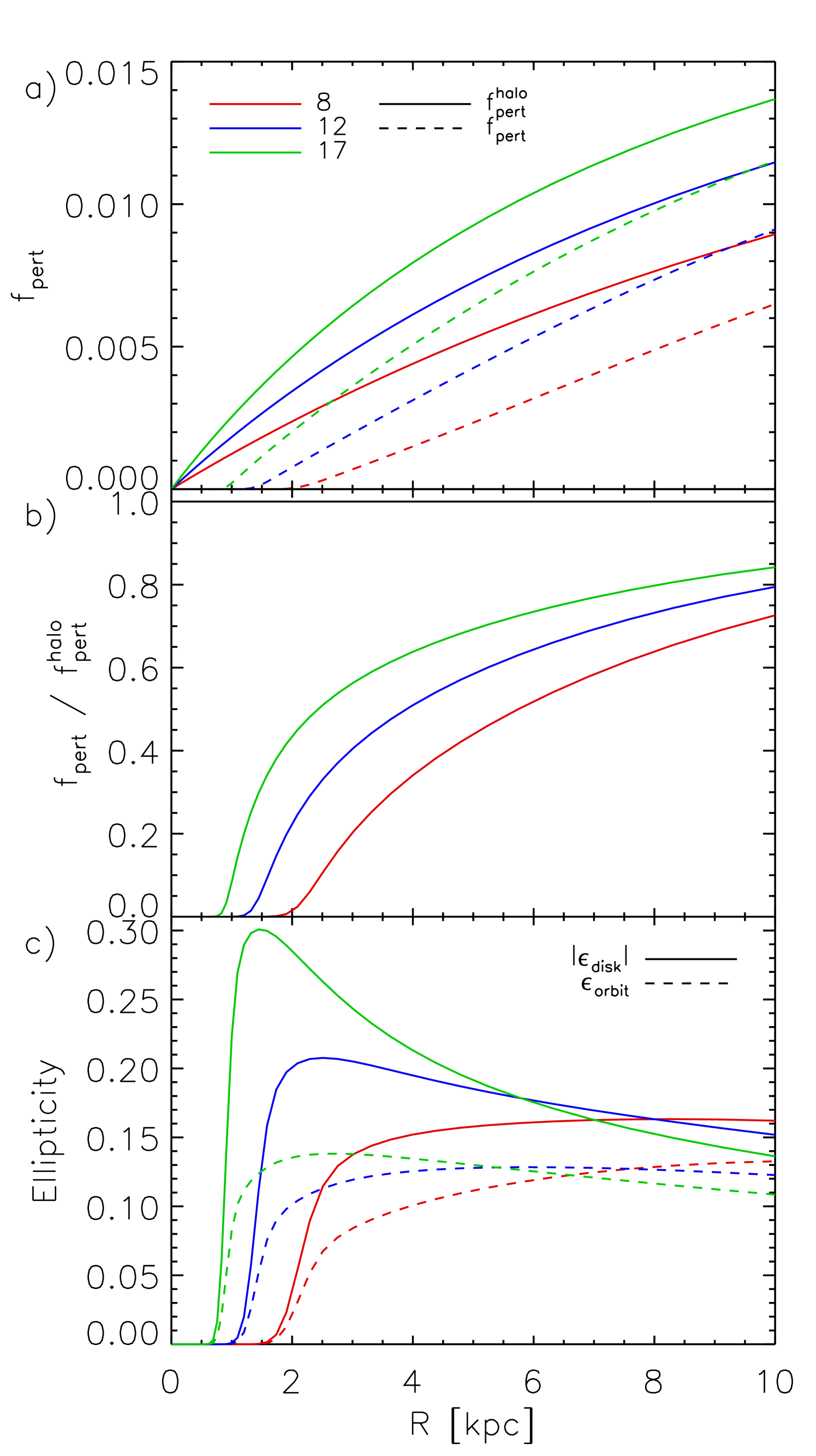
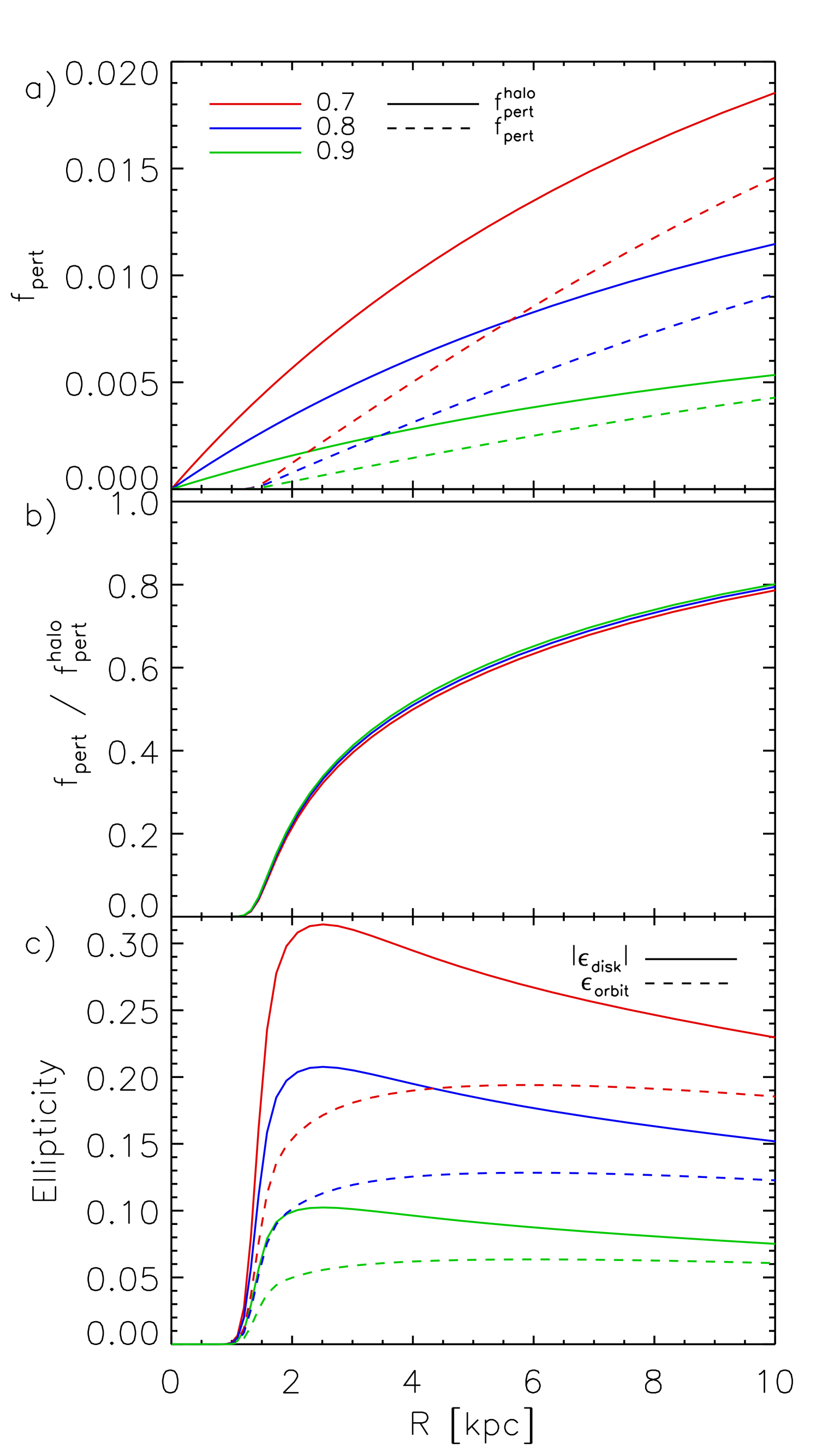
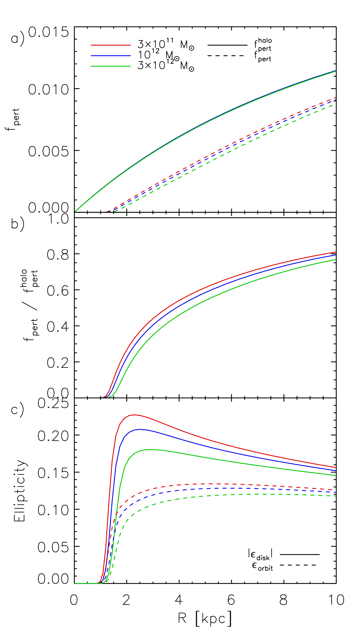
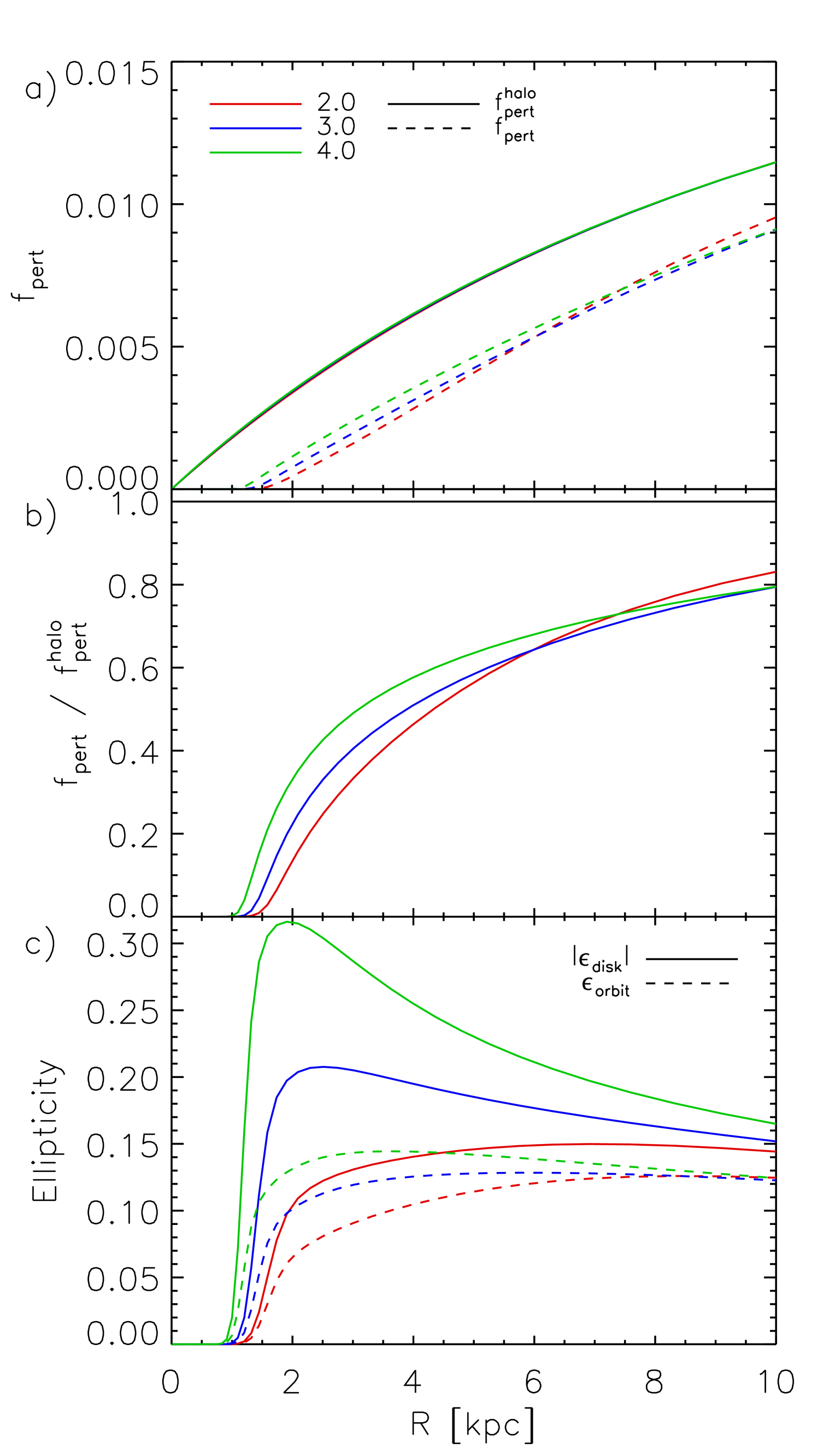
In order to investigate how other properties of the halo and disk affect our results, we have recalculated the results of § 3.1 (where the halo axis ratio was assumed to be constant with radius) for the $3\times 10^{9}~{\mathrm{M}_{\sun}}$ disk while varying the halo concentration, the $b/a$ axis ratio, the halo mass, and the disk scale length. In more concentrated halos (Figure 6), the strength of the perturbation due to the halo, $f_{\mathrm{pert}}^{\mathrm{halo}}$, is larger. The disk is also less able to dilute the perturbation in more concentrated halos. The axis ratio of the halo (Figure 7) has a strong effect on the magnitude of the perturbation but has virtually no effect on the degree to which the disk dilutes the perturbation. In Figure 8 we compare halos of different virial mass, $M_{200}$. In order to facilitate comparison between systems of different mass, we have kept $r_{s}$ constant by varying $c_{200}$ in proportion to $r_{200}$ and kept the relative mass of the disk and halo constant. We find that the mass of the halo has little effect on the relative strength of the perturbation (either before or after the disk is taken into account), but that the resulting disk ellipticities are higher in lower mass systems. Finally, although the equilibrium shape of the potential is similar regardless of the disk scale length (Figure 9), a greater ellipticity is required to achieve this reduction in the perturbation for less concentrated disks, i.e. those with larger scale lengths.

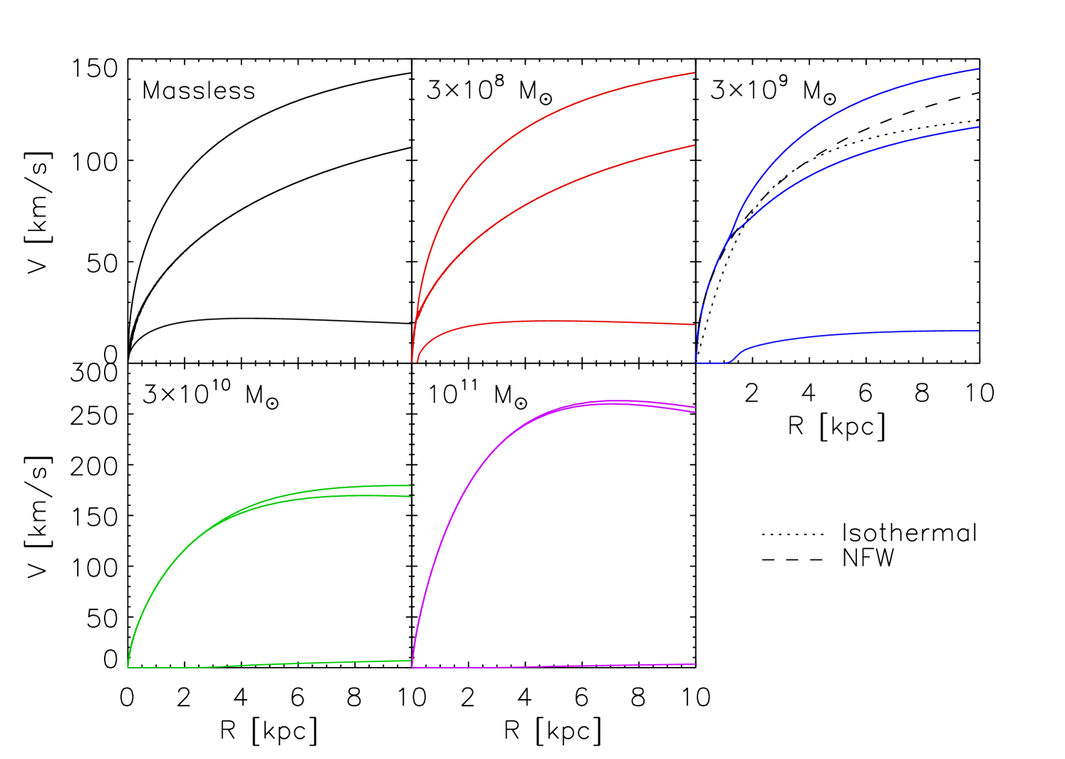
In Figure 10, we plot the azimuthal velocities along the major and minor axes of the halo within the disk plane for disks of different mass in the fiducial sample halo studied in § 3. Full analysis of the velocity fields of these disks will be presented in a future paper. However, we note that none of these rotation curves shows the linear rise characteristic of a constant density core, as expected given the dramatic difference between the form of $f_{\mathrm{pert}}$ in these disks and the form of $f_{\mathrm{iso}}$ required by HN06.

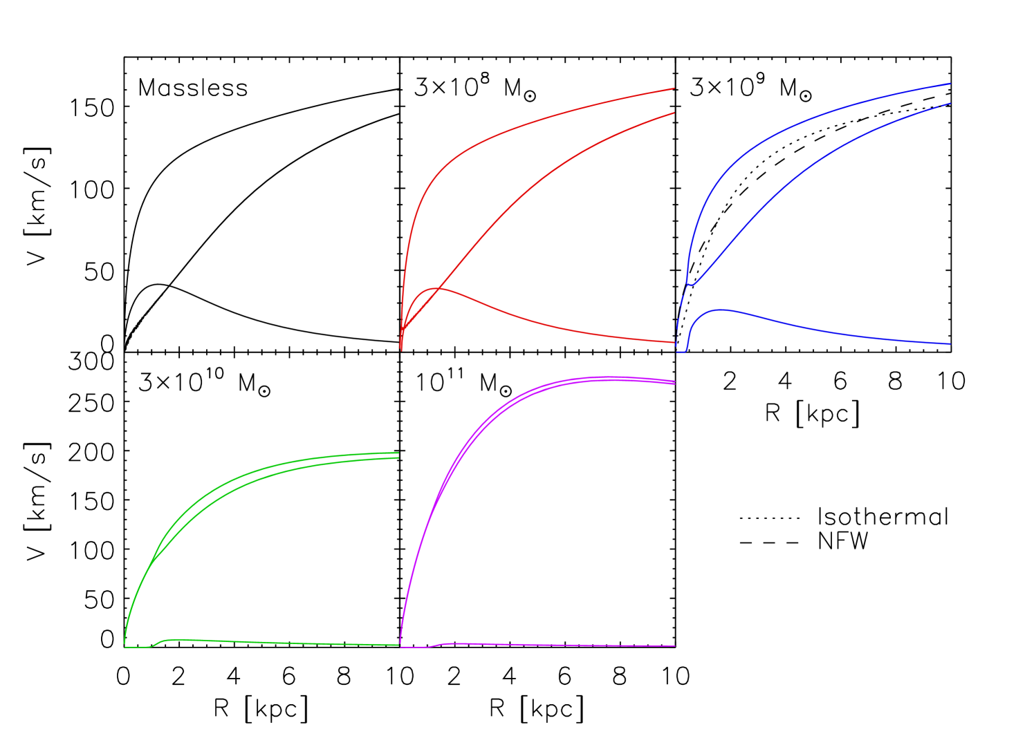
If we use the radial variation of the shape of the halo potential proposed by HNS (Figure 11), for which $f_{\mathrm{pert}}^{\mathrm{halo}}$ is much more similar to $f_{\mathrm{iso}}$, we find that for very low disk masses the azimuthal velocity along the minor axis of the halo is characterized by a much more gradual rise. Observationally, such a rotation curve might be interpreted as indicating a constant-density core in the dark matter halo. However, for disk masses above $3\times 10^{9}~{\mathrm{M}_{\sun}}$ ($0.3\%$ of the virial mass of the halo and just $1.8\%$ of the baryonic mass of the system) the response of the disk removes this feature from the center of the rotation curve. Based on these results, we conclude that simple analyses of the shapes of halos are therefore not sufficient to determine whether halo triaxiality can reconcile LSB rotation curves with cuspy halo density profiles, as suggested by HN06; full analyses that take into account the disk response are required. Preliminary tests on simulated velocity fields constructed using the results of this paper do suggest that triaxiality can produce apparent constant-density cores, in agreement with HN06, but a more detailed analysis including many halos and lines of sight is needed before comparing to the observational distribution of density profile slopes (Simon et al., 2005).

We also plot the maximum radial velocity (amplitude of non-circular motions) at each radius in Figures 10 and 11. Although the radial velocities are much smaller than the azimuthal velocities in all but the lowest mass disks, they are at a level that can be detected in observations of two dimensional velocity fields. The magnitude of the radial motions, which reach $5$–$35~\mathrm{km~s^{-1}}$ depending on the disk mass and halo properties, are consistent with the magnitude of radial motions found by Simon et al. (2005), and reproduce the observed trend for the radial motions to be negligible at small radii and to only become important at larger radii.

It is interesting to compare the ellipticity of our model disks to observed values. Using two-dimensional velocity fields, Simon et al. (2005) found lower limits on the orbital ellipticities ranging from $0$ up to $0.175$, similar to the orbital ellipticities in our model disks. We note that the orbital ellipticity throughout most of the disk is determined by the mass of the disk (Figure 4c), the ellipticity of the halo (Figure 7c), and the variation of halo ellipticity with radius (compare Figures 4c and 5c), with very little dependence on the concentration of either the halo (Figure 6c) or the disk (Figure 9c), or on the global mass of the system (Figure 8c). We therefore predict that galaxies with large observed ellipticities such as NGC 4605 (catalog ) either lie in halos that are more triaxial than average near their center, or contain an unusually low fraction of their mass in their disk. The trends in intrinsic disk ellipticity that we predict may be tested with further analysis of larger kinematic samples, such as those presented by Ganda et al. (2006).

Ryden (2006) found that the distribution of isophotal shapes of galaxies in the 2MASS Large Galaxy Atlas (Jarrett et al., 2003), as measured in the near-infrared $K_{s}$ band (which is a good tracer of the stellar disk mass), is well fit if the intrinsic disk ellipticity distribution is a truncated Gaussian centered at $0.01$ with a width of $\sigma=0.26$. This corresponds to a median ellipticity of $0.18$, with 68% of disks having ellipticities $0.05\leq{\epsilon_{\mathrm{disk}}}\leq 0.37$. For the disk parameters we have studied, the $18.8~\mathrm{mag~arcsec^{-2}}$ isophote at which her shapes were measured corresponds to radii of between $1.5$ and $8.5~\mathrm{kpc}$. Our models naturally produce disk ellipticities in this range at these radii, although the highest ellipticities can only be produced by our least massive disks in our most elliptical potentials.

Finally, we note that our models only take into account ellipticity in the disk induced by the dark matter halo. Central regions of the disk, which have high surface density and sit in an axisymmetric potential, may be unstable to bar formation (Berentzen & Shlosman, 2006). This can induce additional ellipticity to the kinematic and photometric properties of disk galaxies (e.g., Valenzuela et al., 2007).

References

- Allgood et al. (2006) Allgood, B., Flores, R. A., Primack, J. R., Kravtsov, A. V., Wechsler, R. H., Faltenbacher, A., & Bullock, J. S. 2006, MNRAS, 367, 1781
- Bailin et al. (2005) Bailin, J. et al. 2005, ApJ, 627, L17
- Bailin & Steinmetz (2005) Bailin, J., & Steinmetz, M. 2005, ApJ, 627, 647
- Berentzen & Shlosman (2006) Berentzen, I., & Shlosman, I. 2006, ApJ, 648, 807
- Binney & Tremaine (1987) Binney, J., & Tremaine, S. 1987, Galactic dynamics (Princeton University Press)
- de Blok et al. (2001) de Blok, W. J. G., McGaugh, S. S., Bosma, A., & Rubin, V. C. 2001, ApJ, 552, L23
- Dubinski (1994) Dubinski, J. 1994, ApJ, 431, 617
- El-Zant (2001) El-Zant, A. A. 2001, Ap&SS, 276, 1023
- Freeman (1970) Freeman, K. C. 1970, ApJ, 160, 811
- Ganda et al. (2006) Ganda, K., Falcón-Barroso, J., Peletier, R. F., Cappellari, M., Emsellem, E., McDermid, R. M., de Zeeuw, P. T., & Carollo, C. M. 2006, MNRAS, 367, 46
- Gerhard & Vietri (1986) Gerhard, O. E., & Vietri, M. 1986, MNRAS, 223, 377
- Hayashi & Navarro (2006) Hayashi, E., & Navarro, J. F. 2006, MNRAS, 373, 1117 (HN06)
- Hayashi et al. (2007) Hayashi, E., Navarro, J. F., & Springel, V. 2007, MNRAS, in press, astro-ph/0612327 (HNS)
- Jarrett et al. (2003) Jarrett, T. H., Chester, T., Cutri, R., Schneider, S. E., & Huchra, J. P. 2003, AJ, 125, 525
- Jing & Suto (2002) Jing, Y. P., & Suto, Y. 2002, ApJ, 574, 538
- Jog (1997) Jog, C. J. 1997, ApJ, 488, 642
- Jog (1999) —. 1999, ApJ, 522, 661
- Jog (2000) —. 2000, ApJ, 542, 216 (J2K)
- Kazantzidis et al. (2004) Kazantzidis, S., Kravtsov, A. V., Zentner, A. R., Allgood, B., Nagai, D., & Moore, B. 2004, ApJ, 611, L73
- Navarro et al. (1996) Navarro, J. F., Frenk, C. S., & White, S. D. M. 1996, ApJ, 462, 563 (NFW)
- Rix & Zaritsky (1995) Rix, H.-W., & Zaritsky, D. 1995, ApJ, 447, 82
- Ryden (2006) Ryden, B. S. 2006, ApJ, 641, 773
- Schoenmakers et al. (1997) Schoenmakers, R. H. M., Franx, M., & de Zeeuw, P. T. 1997, MNRAS, 292, 349
- Simon et al. (2005) Simon, J. D., Bolatto, A. D., Leroy, A., Blitz, L., & Gates, E. L. 2005, ApJ, 621, 757
- Valenzuela et al. (2007) Valenzuela, O., Rhee, G., Klypin, A., Governato, F., Stinson, G., Quinn, T., & Wadsley, J. 2007, ApJ, 657, 773
- Warren et al. (1992) Warren, M. S., Quinn, P. J., Salmon, J. K., & Zurek, W. H. 1992, ApJ, 399, 405
Appendix A Second-order terms and m=4 distortions
We have assumed that the halo perturbation and the induced distortion in the disk are completely described by the mode. This a direct consequence of only including terms linear in the small quantities , , and their derivatives.
The validity of this assumption can be tested by evaluating the magnitude of the second-order terms that contribute to the distortion in the disk. If we expand the potential as