Self-Knowledge Distillation via Dropout

Hyoje Lee, Yeachan Park, Hyun Seo, Myungjoo Kang
Seoul National University
{hyoje42, ychpark, hseo0618, mkang}@snu.ac.kr

Abstract

To boost the performance, deep neural networks require deeper or wider network structures that involve massive computational and memory costs. To alleviate this issue, the self-knowledge distillation method regularizes the model by distilling the internal knowledge of the model itself. Conventional self-knowledge distillation methods require additional trainable parameters or are dependent on the data. In this paper, we propose a simple and effective self-knowledge distillation method using a dropout (SD-Dropout). SD-Dropout distills the posterior distributions of multiple models through a dropout sampling. Our method does not require any additional trainable modules, does not rely on data, and requires only simple operations. Furthermore, this simple method can be easily combined with various self-knowledge distillation approaches. We provide a theoretical and experimental analysis of the effect of forward and reverse KL-divergences in our work. Extensive experiments on various vision tasks, i.e., image classification, object detection, and distribution shift, demonstrate that the proposed method can effectively improve the generalization of a single network. Further experiments show that the proposed method also improves calibration performance, adversarial robustness, and out-of-distribution detection ability.

1 Introduction

Deep neural networks (DNN) have achieved a state-of-the-art performance in many domains, including image classification, object detection, and segmentation [38, 17, 16]. In designing models that are deeper and more complex for a higher performance, model compression is essential in delivering a deep learning model for practical application. To develope lightweight models, many previous attempts have been made, including an efficient architecture [21, 39], model quantization [10], pruning [14], and knowledge distillation [20].

Although knowledge distillation is a popular DNN compression method, conventional offline knowledge distillation methods have several limitations. To distill the knowledge from a teacher network to a student network, two main steps are required. First, we train a large teacher network, followed by a student network using distillation. Fully training the teacher model with massive datasets requires considerable effort. Second, it is difficult to search for an appropriate teacher model that corresponds to the target student model. In addition, The common belief in traditional knowledge distillation is to expect a larger or more accurate teacher network to be a good teacher. However, a teacher network with a deeper structure and higher accuracy does not guarantee the improved performance of the student network [4, 45].

Self-knowledge distillation is a solution to these limitations. In a self-knowledge distillation, a teacher network becomes a student network itself. Knowledge is efficiently distilled in a single training process in a single model without the guidance of other external models. Several self-distillation methods have been proposed [49, 43, 48, 46]. However, these methods also have the following drawback: 1) Some methods require subnetworks with additional parameters. 2) Some methods request additional ground-truth label information, which means that the model depends on the class distribution of the training datasets.

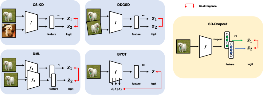
Inspired by these observations, we propose a simple self-knowledge distillation using a dropout (SD-Dropout). Our method generates ensemble models with identical architecture, but different weights through a dropout sampling. After all feature extraction layers, we sample the global feature vector to obtain two different features with different perspectives. These two feature vectors are then passed to the last fully connected layer, and two different posterior distributions are generated. We then match these posterior distributions using Kullback-Leibler divergence (KL-divergence). Dark knowledge between these two internal models can improve their performance through knowledge distillation [20].

The proposed method does not require any additional parameters nor does it require additional label information. For these reasons, SD-Dropout is computationally more efficient than other self-distillation methods. Furthermore, the SD-Dropout method is model-agnostic and method-agnostic, meaning it can be easily implemented with various backbone models and other self-distillation methods.

For more effective distillation, we consider the way to use KL-divergence. In most of the other methods, the gradient of the reference distribution in the KL-divergence is not propagated through model parameters (forward direction of KL divergence). We propose a new approach of utilizing the reverse direction of KL divergence by propagating the gradient flow of the reference distribution. We theoretically demonstrate that the gradient of the reference distribution is greater than that of the other distribution, and we empirically verify the effectiveness of using the gradient of both distributions in the KL-divergence.

We conduct extensive experiments to verify the effectiveness and generalization of our method on various image classification tasks, CIFAR-100 [24], CUB-200-2011 [41], and Stanford Dog [23]. Also, we verify that our method works well on the large-scale dataset, ImageNet [6], and the distribution shift dataset CIFAR-C dataset [18]. We also examine that the proposed method improves the performance in the object detection on the MS COCO dataset [28]. In addition, when acquiring two different sampled feature vectors, only a dropout layer is used after obtaining the feature vectors; thus, the proposed method can be easily applied to any network architecture structure and any knowledge distillation methods.

Experimental results demonstrate that our simple and effective regularization method improves the performance of various model architectures, ResNet [17] and DenseNet [22], and is in good agreement with other knowledge distillation methods [49, 43, 48, 46]. Furthermore, our experiments show that our method improves the calibration performance, adversarial robustness, and out-of-distribution detection ability.

Our contributions are summarized as follows:

•

We present a simple self-knowledge distillation methodology using dropout techniques.
•

Our self-knowledge distillation method can collaborate easily with other knowledge distillation methods.
•

We describe experimental observations regarding the forward and reverse KL-divergence commonly used in knowledge distillation.
•

Extensive experiments demonstrate the effectiveness of our methodology.

2 Related Work

Knowledge distillation [20] is a learning method for transferring knowledge from a large and complex network (known as a teacher network) into a small and simple network (known as a student network). A number of variants have been proposed, inspired by the original method of knowledge distillation, such as the previously mentioned teacher-student framework [35, 19, 31].

On the other hand, research that breaks away from the aforementioned teacher-student framework has been proposed. Deep Mutual Learning (DML) [49] is a distillation method in which a teacher network and a student network distill the knowledge from each other. Data-Distortion Guided Self-Distillation (DDGSD) [43] distills knowledge between different distorted data. Be Your Own Teacher (BYOT) [48] distills knowledge between its deeper and shallow layers. Class-wise self-knowledge distillation (CS-KD) [46] matches the posterior distributions of a model between intra-class instances. We visualize these prior methods in diagram forms in Figure 1.

Refer to caption — Figure 1: Design of the Self-Knowledge Distillation Methods. (Left Blue Background) The designs of existing self-knowledge distillation method. (Right Yellow Background) Our method, SD-Dropout, samples the global feature vector to obtain different features using dropout. These two different features induce different two posterior distributions. The knowledge between the two distributions is distilled to each other. Red arrows indicate distillation using KL-divergence.

These methods have attempted to distill the knowledge from a network within itself. Note that prior methods require subnetworks with additional parameters or request additional label information. Also, some research requires an additional procedure to distort the input data. We remark that these methods are computationally expensive by training additional networks from scratch or traversing two instances from the beginning to the end of a network, and these points are different from ours.

Similar to our work, several semi-supervised and self-supervised learning methods have been investigated. Several studies attempt to solve the semi-supervised task using past selves as teacher networks [25, 40]. Our method and the self-supervised literature [15, 2, 12, 3, 9, 47] have a similar idea of comparing two representations, however, ours does not require augmentations of the input data and additional modules with parameters. The idea of distillation from the ensemble of model for uncertainty estimation is also investigated [26, 8, 30, 29].

We remark that there are several works on knowledge distillation related to dropout. Specifically, there are several works that distill the output from Monte Carlo dropout techniques [1, 13]. These methods investigate distilling the knowledge obtained from averaging Monte Carlo samples into the student model to distill uncertainty. However, these approaches attempt to train the model by mimicking the ensembled prediction obtained by multiple Monte Carlo sampling, we focus on distilling knowledge between internal features obtained from dropout sampling within the model.

3 Self Distillation via Dropout

Throughout this study, we focus on supervised classification tasks. We denote $\mathbf{x}\in\mathcal{X}$ as the input data and $y\in\mathcal{Y}=\{1,2,...,N\}$ as its ground-truth label class. Let $f(\mathbf{x})$ be a global feature vector of the input data $\mathbf{x}$ , and let $h(\cdot)$ be the last fully connected layer in a network. Now, we define $\mathbf{z}=\mathcal{M}_{\theta}(\mathbf{x})=h(f(\mathbf{x}))$ as the logit of the output layer, where $\mathcal{M}_{\theta}$ is the neural network parametrized by $\theta$ . In classification tasks, neural networks typically use a softmax classifier to produce class posterior probability. Thus, we can consider that the posterior probability of class $i$ is as follows:

p(y=i|\mathbf{x};\theta,T)=\frac{exp(z^{i}/T)}{\sum_{j}^{N}{exp(z^{j}/T)}},

(1)

where $z^{i}$ as the logit of class $i$ and $T>0$ is the temperature, which is usually set to 1. In knowledge distillation, the temperature $T$ is set to greater than 1.

3.1 Method Formulation

In this section, we introduce a new self-knowledge distillation method called SD-Dropout. We use the dropout layer after all feature extraction layers. We define

\mathcal{M}^{\mathbf{u}}_{\theta}(\mathbf{x})=h(\mathbf{u}\odot f(\mathbf{x}))\qquad\textrm{where $u^{j}$ $\sim$ Bernoulli($\beta$)}

(2)

where $\odot$ is the element-wise product, and $\beta$ is the dropout rate. Now, $\mathcal{M}^{u}_{\theta}$ is the neural network using a dropout and it produces the posterior probability $p(y|\mathbf{x};\mathbf{u},\theta,T)$ . For brevity, we denote $p^{\mathbf{u}}_{\theta}(y|\mathbf{x}):=p(y|\mathbf{x};\mathbf{u},\theta,T)$ . Similarly, we can also extract an additional feature vector $\mathbf{v}\odot f(\mathbf{x})$ , where $v^{j}$ $\sim$ Bernoulli( $\beta$ ). Thus, we can define $p^{\mathbf{v}}_{\theta}(y|\mathbf{x})$ .

We propose a new regularization loss to distill knowledge by reducing the KL-divergence between two logits $\mathcal{M}^{\mathbf{u}}_{\theta}(\mathbf{x})$ and $\mathcal{M}_{\theta}^{\mathbf{v}}(\mathbf{x})$ . Our method is visualized in Figure 1. This method has computational advantages because, unlike conventional methods, it uses a single existing model, does not require additional modules, shares an encoder, and only requires post fully connected layer operations. Because the two features have no superior relationship with each other, we use this loss in a symmetric manner.

As a result, we use the forward and reverse KL-divergence of both instances. Further discussion on this matter is provided in Section 3.3. Formally, given an input data $\mathbf{x}$ , label $y$ , and randomly dropped operations $\mathbf{u},\mathbf{v}$ , the loss of the SD-Dropout method is defined as follows:

	$\displaystyle\mathcal{L}_{SDD}(\mathbf{x};\mathbf{u},\mathbf{v},\theta,T):={}$	$\displaystyle D_{KL}(p^{\mathbf{u}}_{\theta}(y\|\mathbf{x})\|\|p^{\mathbf{v}}_{\theta}(y\|\mathbf{x}))$		(3)
		$\displaystyle+D_{KL}(p^{\mathbf{v}}_{\theta}(y\|\mathbf{x})\|\|p^{\mathbf{u}}_{\theta}(y\|\mathbf{x}))$		(3)

Our method matches the predictions of different dropout features from a single network, whereas the conventional knowledge distillation method matches predictions from a teacher and a student network. Thus, the total loss $\mathcal{L}_{Total}$ is defined as follows:

	$\displaystyle\mathcal{L}_{Total}(\mathbf{x},y;\mathbf{u},\mathbf{v},\theta,T)={}$	$\displaystyle\mathcal{L}_{CE}(\mathbf{x},y;\;\theta)$		(4)
		$\displaystyle+\lambda_{SDD}\cdot T^{2}\cdot\mathcal{L}_{SDD}(\mathbf{x};\mathbf{u},\mathbf{v},\theta,T)$		(4)

where $\mathcal{L}_{CE}$ is the cross-entropy loss and $\lambda_{SDD}$ is the weight hyperparameter of the SD-Dropout method.

3.2 Collaboration with other method

Our method can easily collaborate with various self-knowledge distillation methods because it has no additional module or training scheme constraints. In collaboration, the loss can be described as Eq. (5), where $\mathcal{L}_{KD}$ is an additional self-knowledge distillation loss for collaboration.

$\displaystyle\mathcal{L}_{Total}(\mathbf{x},y;\mathbf{u},\mathbf{v},\theta,T)={}$	$\displaystyle\mathcal{L}_{CE}(\mathbf{x},y;\;\theta)$	(5)
	$\displaystyle+\lambda_{SDD}\cdot T^{2}\cdot\mathcal{L}_{SDD}(\mathbf{x};\mathbf{u},\mathbf{v},\theta,T)$
	$\displaystyle+\lambda_{KD}\cdot T^{2}\cdot\mathcal{L}_{KD}(\mathbf{x};\theta,T)$

where $\lambda_{KD}$ is the weight hyperparameter of the other distillation methods. The discussion of the appropriate $\lambda_{KD}$ value is detailed in Appendix A.1.

3.3 Forward versus Reverse KL-Divergence

Let $p_{\theta}(\mathbf{x})$ and $q_{\theta}(\mathbf{x})$ be the probability distributions. Let $N$ denote the size of input vector $\mathbf{x}$ . Then, two kinds of KL-divergence, forward and reverse KL-divergence, are defined as follows:

	$\displaystyle D_{KL}^{fw.}(p_{\theta},q_{\theta})=D_{KL}(p\|\|q_{\theta})+D_{KL}(q\|\|p_{\theta})$		(6)
	$\displaystyle D_{KL}^{rv.}(p_{\theta},q_{\theta})=D_{KL}(p_{\theta}\|\|q)+D_{KL}(q_{\theta}\|\|p)$		(7)

Note that the absence of $\theta$ in $p$ indicates that $p$ is considered constant with respect to $\theta$ , meaning that the gradient is not propagated.

In the field of knowledge distillation, it is widely accepted that the forward KL-divergence is based on similarity with the Cross-Entropy loss. That is, the features of the teacher network are considered as the ground-truth, and the features of the student network are considered as logits that approximate the features of the teacher networks. However, we also adopt a reverse KL-divergence direction to further reduce the divergence between the two distributions.

The idea of utilizing reverse direction is also proposed as a new loss approximating the target Dirichlet distribution in [29]. Since forward KL divergence is zero-avoiding, utilizing only the forward direction is not suitable if the target Dirichlet distribution is multi-modal. We extend the analysis of the direction of KL divergence to the general distribution settings.

We claim that the derivative of reverse divergence is stronger than that of forward divergence. We show this by proving Proposition 1 with analysis presented below. This indicates that the reverse direction is not negligible and plays an important role. In addition, we claim that the forward and reverse KL divergence work differently, in other words, their directions of the derivatives are quite different. We empirically verify this claim in Section 4.6.1. Overall, by adding reverse divergence, we expect stronger self-knowledge distillation.

First, we observe the representation of the derivatives of forward and reverse KL-divergence.

Lemma 1.

The derivatives of forward and reverse divergence is represented as follows:

\nabla_{\theta}D_{KL}^{fw.}(p_{\theta},q_{\theta})=\sum_{i=1}^{N}(1-\frac{p(\mathbf{x})_{i}}{q(\mathbf{x})_{i}})\nabla_{\theta}q(\mathbf{x})_{i}+\sum_{i=1}^{N}(1-\frac{q(\mathbf{x})_{i}}{p(\mathbf{x})_{i}})\nabla_{\theta}p(\mathbf{x})_{i}

(8)

\nabla_{\theta}D_{KL}^{rv.}(p_{\theta},q_{\theta})=\sum_{i=1}^{N}\log(\frac{p(\mathbf{x})_{i}}{q(\mathbf{x})_{i}})\nabla_{\theta}p(\mathbf{x})_{i}+\sum_{i=1}^{N}\log(\frac{q(\mathbf{x})_{i}}{p(\mathbf{x})_{i}})\nabla_{\theta}q(\mathbf{x})_{i}

(9)

Before beginning the main proposition, we make the following assumptions.

Assumption 1.

If $|p(\mathbf{x})_{i}|>|q(\mathbf{x})_{i}|,$ then $|\nabla_{\theta}p(\mathbf{x})_{i}|>|\nabla_{\theta}q(\mathbf{x})_{i}|$ . If $|p(\mathbf{x})_{i}|<|q(\mathbf{x})_{i}|$ , then $|\nabla_{\theta}p(\mathbf{x})_{i}|<|\nabla_{\theta}q(\mathbf{x})_{i}|$ . $\textit{i.e.},(|\frac{p(\mathbf{x})_{i}}{q(\mathbf{x})_{i}}|-1)(|\frac{\nabla_{\theta}p(\mathbf{x})_{i}}{\nabla_{\theta}q(\mathbf{x})_{i}}|-1)>0.$

Assumption 2.

Let $r=\log(|\frac{p(\mathbf{x})_{i}}{q(\mathbf{x})_{i}}|)$ and $\rho=|\frac{\nabla_{\theta}p(\mathbf{x})_{i}}{\nabla_{\theta}q(\mathbf{x})_{i}}|>1$ . Then $r\leq r_{1}$ where $r_{1}=|\log(\rho)+\log(\log(\rho+(e-1)))|$ .

Assumption 1 implies that if $|p(\mathbf{x})|$ is greater than $|q(\mathbf{x})|$ , then the derivative $\nabla_{\theta}p(\mathbf{x})$ is also greater than $\nabla_{\theta}q(\mathbf{x})$ . Assumption 2 implies that the ratio $|\frac{p(\mathbf{x})}{q(\mathbf{x})}|$ is not significantly different from the ratio $|\frac{\nabla_{\theta}p(\mathbf{x})}{\nabla_{\theta}q(\mathbf{x})}|$ . We empirically validate that Assumptions 1 and 2 hold in probability during the experiment. Now, we posit the main proposition indicating that the reverse derivative is greater than the forward derivative under Assumptions 1 and 2. In other words, we can demand a stronger connectedness (or bond) between logits $p(\mathbf{x})$ and $q(\mathbf{x})$ in the training process by adding reverse derivatives.

Proposition 1.

Under Assumptions 1 and 2, let :

	$\displaystyle(D_{i,\theta})$	$\displaystyle=\|\log(\frac{p(\mathbf{x})_{i}}{q(\mathbf{x})_{i}})\nabla_{\theta}q(\mathbf{x})_{i}\|+\|\log(\frac{q(\mathbf{x})_{i}}{p(\mathbf{x})_{i}})\nabla_{\theta}p(\mathbf{x})_{i}\|$
	$\displaystyle-$	$\displaystyle(\;\|(1-\frac{p(\mathbf{x})_{i}}{q(\mathbf{x})_{i}})\nabla_{\theta}q(\mathbf{x})_{i}\|+\|(1-\frac{q(\mathbf{x})_{i}}{p(\mathbf{x})_{i}})\nabla_{\theta}p(\mathbf{x})_{i}\|\;)$		(10)

Then we have:

(D_{i,\theta})>0.

(11)

Moreover, $(D_{i})$ has a maximum value at $r=|\log(\rho)|$ . Here, $(D_{i})$ implies the difference between the $L_{1}$ norm of the reverse derivatives and the $L_{1}$ norm of the forward derivatives.

We present the detailed proofs of the above proposition in the supplementary materials.

Table 1: Accuracy (%) of self-knowledge distillation methods on CIFAR-100, CUB-200-2011, and Stanford Dogs datasets. Best results are indicated in bold.

Method	CIFAR-100		CUB-200-2011		Standford Dogs
Method	Base	+SD-Dropout	Base	+SD-Dropout	Base	+SD-Dropout
Cross-Entropy	74.8	77.0 (+2.2)	53.8	66.6 (+12.8)	63.8	69.9 (+6.1)
CS-KD	77.3	77.4 (+0.1)	64.9	65.4 (+0.6)	68.8	69.3 (+0.5)
DDGSD	76.8	77.1 (+0.3)	58.3	62.9 (+4.6)	66.9	68.1 (+1.3)
BYOT	77.2	77.7 (+0.5)	60.6	68.7 (+8.1)	68.7	71.2 (+2.5)
DML	78.9	78.8 (-0.1)	61.5	65.7 (+4.2)	70.5	72.0 (+1.6)
LS	76.8	76.9 (+0.1)	56.2	67.6 (+11.5)	65.2	70.1 (+4.9)

4 Experiments

In this section, we present the effectiveness of the proposed method. We demonstrate our method on a variety of tasks including image classification, object detection, calibration effect, robustness, and out-of-distribution detection. In addition, we conduct extensive experiments on the direction of KL-divergence, backbone networks, comparison with standard dropout, and generalizability of our method.

Throughout this section, we use ResNet-18 or its variants as the architecture and CIFAR-100 as the training dataset if there is no specific description. All experiments are performed using PyTorch [36].

4.1 Classification

4.1.1 CIFAR-100, CUB200, and Stanford Dogs

Dataset

To validate the general performance of our method, we test various datasets including CIFAR-100 [24], CUB-200-2011 [41], and Stanford Dogs [23]. CIFAR-100 is composed of 100 classes with large contextual differences between classes. By contrast, CUB-200-2011 and Stanford Dogs are composed of 200 and 120 fine-grained classes, and unlike CIFAR-100, there are smaller contextual differences between classes. The Performance in various dataset domains can be used to evaluate the overall performance of the model.

Hyperparameters

For a fair comparison, we use the same hyperparameters in all experiments unless specifically mentioned. We use a stochastic gradient descent optimizer (learning rate=0.1, momentum=0.9, weight decay=1e-4) and train 200 epochs during all experiments. The learning rate is scheduled for decay 0.1 on 100 and 150 epochs. As a common setting for CIFAR-100, we set a batch size of 128 and use ResNet, which modifies the first convolution layer with a 3 $\times$ 3 kernel instead of a 7 $\times$ 7 kernel. We set input image sizes of 224 $\times$ 224 and batch sizes of 32 on CUB-200-2011 and Stanford Dogs. All results are the average values obtained by repeating the experiment three times.

Training Procedure

The training procedure of SD-Dropout is summarized as PyTorch-like style pseudo code, as described in Algorithm 1. It should be noted that we do not use the .detach() method to calculate the KL-divergence terms to maintain both directions of KL-divergence.

⬇

# x: input image

# y: ground-truth label

# backbone : feature extractor composed of convolutions

# classifier : fully connected layer

# lambda: weight hyperparamter of knowledge distillation method

for (x, y) in Batches:

# extract the feature

feat = backbone(x)

# the values of the logits

output = classifier(feat)

# calculate cross-entropy loss

loss_ce = ce_loss(output, y)

# sampling two features by dropout

feat_dps = [dropout(feat) for _ in range(2)]

# the logits of two dropout sampled feature

output_dp1, output_dp2 =

[classifier(feat_dps[i]) for i in range(2)]

# Foward reverse KL-divergence between two logits

loss_kd1 = kl_div_loss(output_dp1, output_dp2)

loss_kd2 = kl_div_loss(output_dp2, output_dp1)

loss_kd = loss_kd1 + loss_kd2

# total loss

loss_total = loss_ce + lambda*loss_kd

# update

loss_total.backward()

Algorithm 1 Pseudo code of SD-Dropout in a PyTorch-like style.

Results

While using the fixed backbone model (ResNet-18), we compare the accuracy of the methods and datasets. Table 1 shows the accuracy on CIFAR-100, CUB-200-2011, and Stanford Dogs in comparison with distillation and regularization methods, i.e., Cross-Entropy, CS-KD, DDGSD, BYOT, DML, and label smoothing (LS). Moreover, the [+ SD-Dropout] column is the result of a collaboration between existing methods. The dropout collaboration improves the performance of all datasets and self-distillation methodologies. Compared to previous self-distillation methods, although simply applicable, the SD-Dropout method performs best on the CUB-200-2011 dataset at 66.6%. Furthermore, the largest increase in the performance showed that the compatibility with BYOT is the best (0.5% on CIFAR-100, 8.1% on CUB-200-2011, and 2.5% on Stanford Dogs).

Table 2: Expected Calibration Error comparison results of SD-Dropout combined with various knowledge distillation methodologies. The trained network is ResNet-18. Lower is better and the best results are indicated in bold.

Method	Base	+SD-Dropout
Cross-Entropy	0.120	0.075
DDGSD	0.067	0.034
CS-KD	0.068	0.046
BYOT	0.117	0.056
DML	0.058	0.039

4.1.2 ImageNet

Table 3: Classification Accuracy (%) on the ImageNet dataset for ResNet-152. Metric is Top-k accuracy (ACC @ k)

Method	Acc @ 1	Acc @ 5
Cross-Entropy	74.8	92.5
SD-Dropout	75.5	92.7

Dataset

To validate our methodology even on the large-scale dataset, we evaluate the classification problem on ILSVRC 2012 dataset [6]. ImageNet is a dataset of 1000 classes of 1.28 million training images and 50k validation images. We evaluate both top-1 and top-5 error rates.

Hyperparameters

The hyperparameters used for learning baseline model and SD-dropout methodologies are as follows. All models are trained for 90 epochs. We use a 32 mini-batch size with a stochastic gradient descent optimizer. The learning rate is scheduled for decay 0.1 on 30 and 60 epochs. We use 1e-4 weight decay and 0.9 momentum. The input image is randomly cropped with 224 $\times$ 224 size and augmented with random horizontal flip. The lambda of the SD-Dropout method is 0.1. All models used the same hyperparameters except for lambda. The learning process is the same as section 4.1.1.

Results

We select the ResNet-152 model as the baseline model to ensure that our method is valid even for the large-scale dataset and large model. Table 3 shows that the accuracy of the SD-Dropout method is better than the result of learning the baseline model with cross-entropy loss. The result implies that SD-Dropout is a universally applicable method for large datasets and large models as well as narrow datasets and small models.

4.2 Object Detection

To verify the effectiveness of SD-Dropout on the visual recognition tasks, we perform the experiment on the task of object detection using the COCO dataset [28]. We use the Faster R-CNN [37] detector with a backbone of ResNet-152 trained on ImageNet as described in Section 4.1.2. We finetune Faster R-CNN for 7 epochs (0.5 $\times$ schedule) and 12 epochs (1 $\times$ schedule). As shown in Table 4, SD-Dropout shows better results in object detection than the baseline. These results indicate that SD-Dropout is successful for transferring to another vision task.

Table 4: Results on object detection. mAP@0.5 denotes mean average precision with IOU threshold 0.5. mAP denotes COCO-style mAP. Best results are indicated in bold.

Method	0.5 $\times$ Schedule	1 $\times$ Schedule
	mAP / mAP@0.5
Cross-Entropy	31.2 / 50.6	39.4 / 60.1
SD-Dropout	32.5 / 52.8	39.8 / 60.7

4.3 Calibration Effect

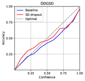
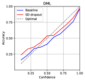
Figure 2: Reliability diagrams [34]. The x-axis is confidence bin and the y-axis is average accuracy on bin. The blue and red line show average accuracy w/ and w/o SD-dropout method.

The expected calibration error (ECE) [32] is a metric that shows the difference between the confidence of the model predictions and the actual accuracy. The ECE can be calculated as

ECE=\sum_{m=1}^{M}\frac{|B_{m}|}{n}\;|acc(B_{m})-conf(B_{m})|,

(12)

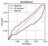
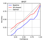
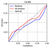
where $M$ , $n$ , $B_{m}$ , $acc(B_{m})$ , and $conf(B_{m})$ denote the number of bins, the number of total samples, the number of samples in the $m$ -th bin, the average accuracy of samples in the bin, and the average model confidence of samples in the bin. We set the number of bins to 10. The results shown in Table 2 and Figure 2 indicate that SD-Dropout suppresses overconfidence and improves confidence calibration.

4.4 Robustnetss

4.4.1 Robustness to adversarial attack

Table 5: Robustness comparison against the adversarial attack. Accuracy (%) of ResNet-18 on various datasets. Best results are indicated in bold.

Dataset	Base	+SD-Dropout
CIFAR-100	37.9	47.1
CUB-200-2011	17.0	24.8
Stanford Dogs	19.2	22.6

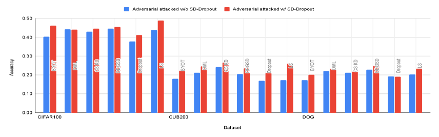
To evaluate the robustness to adversarial attacks [7], we compare the performance of methods subjected to an adversarial attack. An adversarial attack approach is the Fast gradient sign method [11] that exploits the gradient of network with respect to the input image to increase the loss, where the maximum perturbation size is $\epsilon$ = 0.2. The result are reported in Table 5.

As shown in Figure 3, we demonstrate the adversarial robustness with collaborate cases. All results show increases in the robustness of the adversarial attacks. It can be concluded that the SD-Dropout method has an effect similar to that of adversarial training.

4.4.2 Robustness to Distribution Shift

Table 6: Robustness to the distribution shift dataset, CIFAR-C. There are 15 types of corruption. mCA indicates the mean corruption accuracy. The network ResNet-18 is trained by the CIFAR-100 dataset. Best results are indicated in bold.

Corruption		Cross-Entropy	SD-Dropout
Noise	Gauss.	23.1	21.9
	shot	31.2	30.2
	Impulse	27.1	25.4
Blur	Defocus	57.0	59.1
	Glass	25.1	23.1
	Motion	52.4	54.2
	Zoom	50.1	52.9
Weather	Snow	52.7	54.9
	Frost	47.2	48.7
	Fog	61.1	63.3
	Bright	70.2	72.4
Digital	Contrast	50.6	53.6
	Elastic	59.4	60.7
	Pixel	52.9	52.7
	JPEG	52.4	51.2
mCA		47.49	48.28

To evaluate the classification robustness of the distribution shift task, we compare the accuracy of methods on the CIFAR-C dataset [18]. CIFAR-C dataset includes 15 types of corruption from noise, blur, weather, and digital categories. We evaluate the networks trained by the normal CIFAR-100 dataset. In table 6, the average mean corruption accuracy (mCA) of our method outperforms the baseline. In detail, SD-Dropout is better for nine types of corruption, but worse for six types of corruption. As can be seen from the experimental results, SD-Dropout is generally robust in various noise environments of the input images.

4.5 Out-of-Distribution Task

Table 7: Result on the out-of-distribution dataset. The CIFAR-100 dataset is used as an in-distribution dataset.

\uparrow

means larger is better, and

\downarrow

means lower is better. The metrics are explained in Section 4.5. The trained network is ResNet-18. Best results are indicated in bold.

Dataset	FPR	Detection	AUROC	AUPR	AUPR
	(at 95% TPR)	Error	AUROC	(in)	(out)
	$\downarrow$	$\downarrow$	$\uparrow$	$\uparrow$	$\uparrow$
	Cross-Entropy/SD-Dropout (%)
LSUN	74.7/63.5	25.0/22.9	82.0/84.9	84.5/84.8	78.5/83.4
iSUN	76.0/63.8	25.3/23.0	82.0/84.8	85.9/85.6	76.0/81.9
DTD	82.7/77.5	28.6/27.4	77.3/77.2	86.3/83.7	59.8/64.0
SVHN	82.6/75.2	22.7/27.4	82.9/79.1	86.6/78.3	75.5/76.7
Average	79.0/70.0	25.4/25.1	81.1/81.5	85.8/83.1	72.4/76.5

We also validate that our method can detect whether it is an out-of-distribution example. It is important whether our model can predict whether the test examples come from an in-distribution or an out-distribution. To evaluate the performance of out-of-distribution detection, we use the ODIN detector [27]. The ODIN detector can discriminate in-distribution and out-distribution by using temperature scaling and adding small perturbations to a test example. Since the ODIN method does not require any changes to a pre-trained network, we use the baseline and SD-Dropout model as the backbone of the ODIN detector. The other hyper-parameters are set to the same values as the original paper.

We use four following metrics to evaluate the detection performance on in- and out-of-distribution datasets. FPR at 95 % TPR) is the false positive rate (FPR) when the true positive rate (TPR) is 95%. Detection Error is calculated by $0.5\cdot(1-TPR)+0.5\cdot FPR$ . AUROC is the area under the receiver operating characteristic curve. AUPR is the area under the precision-recall curve. We measure AUPR both in- and out-of-distribution dataset, respectively. Here, the in-distribution dataset is the CIFAR-100 datasets. We use LSUN [44], iSUN [42], DTD [5], and SVHN [33] datasets as out-of-distribution datasets.

The result is shown in Table 7. SD-Dropout induces the reduction in the variation of the features sampled by the dropout. As a result, the proposed method reduces the uncertainty of in-distribution dataset. This is similar to a contrastive loss of positive pairs in constrative learning. For this reason, it can be concluded that our method shows superior performance in the out-of-distribution task compared to the cross-entropy.

4.6 Additional Study

4.6.1 Directions of KL-divergence

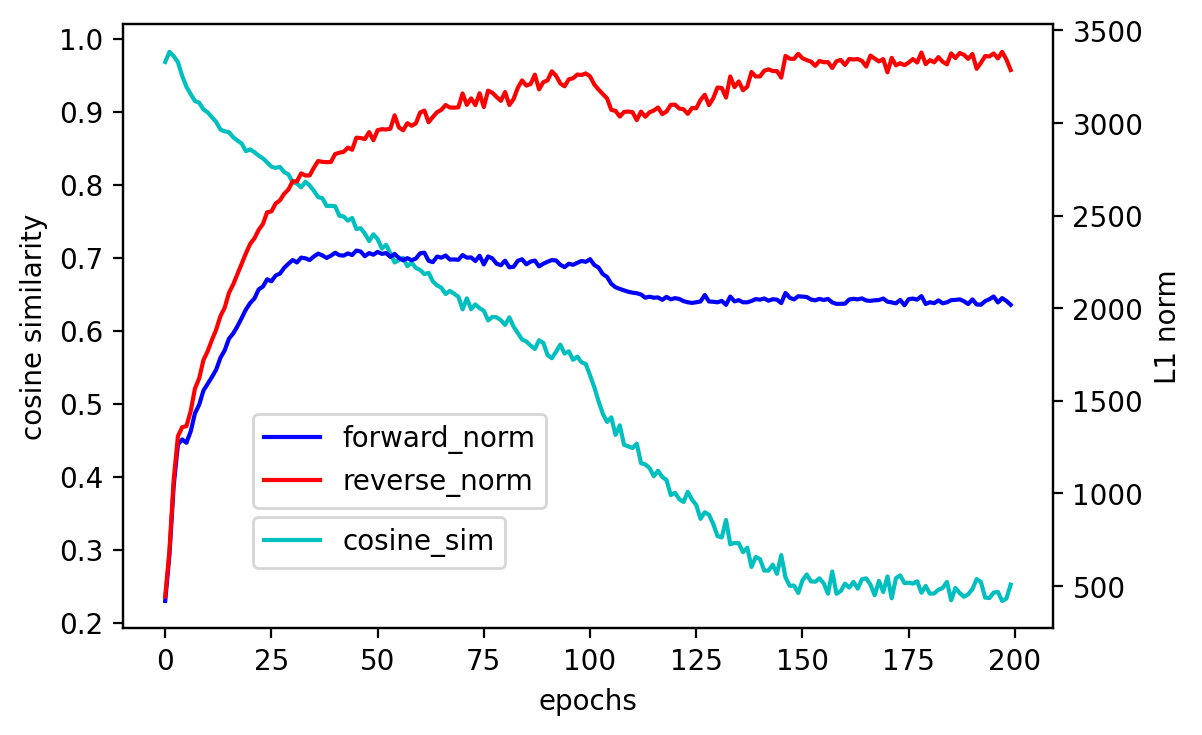
We empirically verify through experiments that Assumptions 1 and 2 in Section 3.3 are convincing (see Table 8). We use ResNet-18 on the CIFAR-100 dataset in the experiment. The probability that Assumption 1 holds is greater than 0.5 in all epoch. $L_{1}$ norm of $r$ in Assumption 2 is smaller than $r_{1}$ in all epochs.

As discussed in Section 3.3, we use both directions of KL divergence. To verify its effectiveness, we conduct an ablation experiment on the directions of KL divergence. As shown in Table 9, the model using both directions of KL-divergence achieves the best performance. In addition, we investigate the directions of the gradient from forward and reverse KL divergence on the CIFAR-100. As shown in Figure 4, the cosine similarity between the gradients in the two directions gradually decreases as training progresses. This indicates that the directions of two gradients are significantly different, and both directions of KL divergence are essential for training. Furthermore, we also see that the $L_{1}$ norm of the gradient from the reverse derivative is greater than the forward derivative, similar to the analysis in Section 3.3.

Table 8: Verification of assumptions in Section 3.3

Epoch	$P$ (Assumption 1)	$r$	$r_{1}$
0	0.638	0.0681	0.1368
100	0.653	0.1403	0.2799
200	0.594	0.1292	0.2662

Table 9: Accuracy (%) comparison between the forward, reverse, and both directions (forward and reverse) of KL-divergence on ResNet-18. Best results are indicated in bold.

Dataset	Base	Forward	Reverse	Both Directions
CIFAR-100	74.8	76.6	76.3	77.0
CUB-200-2011	53.8	65.4	63.8	66.6
Stanford Dogs	64.1	69.6	69.7	69.8

4.6.2 Backbone Network

Table 10: Accuracy (%) comparison with different backbone networks on CIFAR-100. Best results are indicated in bold.

Architecture	Base	+SD-Dropout
ResNet-18	74.8	77.0
ResNet-34	75.7	77.2
DenseNet-121	77.3	78.4

Our self-distillation method is easily adaptable to various backbone models. We compare several backbone networks with and without SD-Dropout. We apply SD-Dropout to ResNet-18, ResNet-34, and DenseNet-121. Table 10 shows that the SD-Dropout method can improve the network performance regardless of the backbone networks. In particular, our SD-Dropout improves the accuracy of the baseline networks from 74.8% to 77.0% for ResNet-18, and from 75.7% to 77.2% for ResNet-34 on the CIFAR-100 dataset. For DenseNet-121, our method enhances the accuracy from 77.3% to 78.4%.

Table 11: Accuracy (%) comparison between standard dropout and SD-Dropout. [standard^†] represents the standard dropout method that equalizes the number of training steps compared to SD-Dropout. Best results are indicated in bold.

Dataset	Base	+Dropout	+Dropout	+SD-Dropout
Dataset	Base	(standard)	(standard^†)	+SD-Dropout
CIFAR-100	74.8	75.4	73.5	77.0
CUB-200-2011	53.8	64.6	60.3	66.6
Stanford Dogs	64.1	69.5	68.0	69.8

Table 12: Accuracy comparison with various positions of dropout on CIFAR-100. The trained network is ResNet-18. Best results are indicated in bold.

Method	Accuracy (%)
Cross-Entropy	74.8
SD-Dropout	77.0
SD-Dropout (after layer1)	74.8
SD-Dropout (after layer2)	75.1
SD-Dropout (after layer3)	75.7

Table 13: Accuracy comparison between networks with multiple fully-connected layers on CIFAR-100. The trained network is ResNet-18 with two fully-connected layers. Best results are indicated in bold.

Method	Accuracy (%)
Cross-Entropy	74.9
SD-Dropout	75.9

4.6.3 Comparison with Standard Dropout

The dropout technique plays the most important role in the SD-Dropout method. To demonstrate the importance of dropout distillation with our method, we compare it with networks using standard dropout methods. Also, we equalize the number of training steps between standard dropout and SD-Dropout methods. Table 11 compares the experimental results of the standard dropout and our SD-Dropout methods on the CIFAR-100, CUB-200-2011, and Stanford Dogs datasets. It is observed that our SD-Dropout method outperforms the standard dropout methods on all datasets.

4.6.4 Dropout at Various Positions

To get various sampled feature vectors, we apply dropout from deep layer to shallow layer. It is important which layer to apply the dropout. While our method applies dropout prior to a fully-connected layer, our method can be generalized and apply dropout to any layer, theoretically. We conduct further experiments from this perspective. In particular, ResNet can be divided into 4 large parts. For convenience, name these parts layer1 $\sim$ 4. That is, our method applies dropout after layer4. In Table 12, we compare the results of methods that apply dropout to a different layer. Although dropouts are applied to different layers, they mostly outperform the baseline cross-entropy method. From the experimental results, the high-level features sampled from the deep layer are more suitable for SD-Dropout than the low-level features sampled from the shallow layer.

4.6.5 Multiple Fully-connected Layers

Our method is model-agnostic, which means it can be applied to any structure of the model. Throughout the paper, we treat the network whose structure is composed of convolutional layers and one fully-connected layer. To show that the SD-dropout method can be applied to any structure, we apply our method to a network with multiple fully-connected layers. We append one additional fully-connected layer with 512 hidden units. The result is in Table 13. It appears that our method also improves the performance of a network with multiple fully-connected layers.

5 Conclusion

We propose a new and simple self-knowledge distillation method. The proposed method samples different models through a dropout and distills the knowledge of both. We also experimentally and analytically show the characteristics of reverse KL-divergence. We demonstrate that the proposed method improves generalization, calibration performance, adversarial robustness, and ability of out-of-distribution detection. From the perspective of the regularization domain, our method is superior to the conventional label smoothing method through multiple datasets. Thus, we expect our method to be used as a regularization method that can effectively improve the performance of a single network in various domains.

References

[1] Samuel Rota Bulò, Lorenzo Porzi, and Peter Kontschieder. Dropout distillation. In International Conference on Machine Learning, pages 99–107. PMLR, 2016.
[2] Ting Chen, Simon Kornblith, Mohammad Norouzi, and Geoffrey Hinton. A simple framework for contrastive learning of visual representations. In International conference on machine learning, pages 1597–1607. PMLR, 2020.
[3] Xinlei Chen and Kaiming He. Exploring simple siamese representation learning. In Proceedings of the IEEE/CVF Conference on Computer Vision and Pattern Recognition, pages 15750–15758, 2021.
[4] Jang Hyun Cho and Bharath Hariharan. On the efficacy of knowledge distillation. In Proceedings of the IEEE/CVF International Conference on Computer Vision, pages 4794–4802, 2019.
[5] Mircea Cimpoi, Subhransu Maji, Iasonas Kokkinos, Sammy Mohamed, and Andrea Vedaldi. Describing textures in the wild. In Proceedings of the IEEE conference on computer vision and pattern recognition, pages 3606–3613, 2014.
[6] Jia Deng, Wei Dong, Richard Socher, Li-Jia Li, Kai Li, and Li Fei-Fei. Imagenet: A large-scale hierarchical image database. In 2009 IEEE Conference on Computer Vision and Pattern Recognition, pages 248–255, 2009.
[7] Yinpeng Dong, Qi-An Fu, Xiao Yang, Tianyu Pang, Hang Su, Zihao Xiao, and Jun Zhu. Benchmarking adversarial robustness on image classification. In Proceedings of the IEEE/CVF Conference on Computer Vision and Pattern Recognition, pages 321–331, 2020.
[8] Erik Englesson and Hossein Azizpour. Efficient evaluation-time uncertainty estimation by improved distillation. arXiv preprint arXiv:1906.05419, 2019.
[9] Spyros Gidaris, Andrei Bursuc, Gilles Puy, Nikos Komodakis, Matthieu Cord, and Patrick Perez. Obow: Online bag-of-visual-words generation for self-supervised learning. In Proceedings of the IEEE/CVF Conference on Computer Vision and Pattern Recognition, pages 6830–6840, 2021.
[10] Yunchao Gong, Liu Liu, Ming Yang, and Lubomir Bourdev. Compressing deep convolutional networks using vector quantization. arXiv preprint arXiv:1412.6115, 2014.
[11] Ian J Goodfellow, Jonathon Shlens, and Christian Szegedy. Explaining and harnessing adversarial examples. arXiv preprint arXiv:1412.6572, 2014.
[12] Jean-Bastien Grill, Florian Strub, Florent Altché, Corentin Tallec, Pierre Richemond, Elena Buchatskaya, Carl Doersch, Bernardo Avila Pires, Zhaohan Guo, Mohammad Gheshlaghi Azar, et al. Bootstrap your own latent-a new approach to self-supervised learning. Advances in neural information processing systems, 33:21271–21284, 2020.
[13] Corina Gurau, Alex Bewley, and Ingmar Posner. Dropout distillation for efficiently estimating model confidence. arXiv preprint arXiv:1809.10562, 2018.
[14] Song Han, Huizi Mao, and William J Dally. Deep compression: Compressing deep neural networks with pruning, trained quantization and huffman coding. arXiv preprint arXiv:1510.00149, 2015.
[15] Kaiming He, Haoqi Fan, Yuxin Wu, Saining Xie, and Ross Girshick. Momentum contrast for unsupervised visual representation learning. In Proceedings of the IEEE/CVF conference on computer vision and pattern recognition, pages 9729–9738, 2020.
[16] Kaiming He, Georgia Gkioxari, Piotr Dollár, and Ross Girshick. Mask r-cnn. In Proceedings of the IEEE international conference on computer vision, pages 2961–2969, 2017.
[17] Kaiming He, Xiangyu Zhang, Shaoqing Ren, and Jian Sun. Deep residual learning for image recognition. In Proceedings of the IEEE conference on computer vision and pattern recognition, pages 770–778, 2016.
[18] Dan Hendrycks and Thomas Dietterich. Benchmarking neural network robustness to common corruptions and perturbations. arXiv preprint arXiv:1903.12261, 2019.
[19] Byeongho Heo, Minsik Lee, Sangdoo Yun, and Jin Young Choi. Knowledge distillation with adversarial samples supporting decision boundary. In Proceedings of the AAAI Conference on Artificial Intelligence, volume 33, pages 3771–3778, 2019.
[20] Geoffrey Hinton, Oriol Vinyals, and Jeff Dean. Distilling the knowledge in a neural network. arXiv preprint arXiv:1503.02531, 2015.
[21] Andrew G Howard, Menglong Zhu, Bo Chen, Dmitry Kalenichenko, Weijun Wang, Tobias Weyand, Marco Andreetto, and Hartwig Adam. Mobilenets: Efficient convolutional neural networks for mobile vision applications. arXiv preprint arXiv:1704.04861, 2017.
[22] Gao Huang, Zhuang Liu, Laurens Van Der Maaten, and Kilian Q Weinberger. Densely connected convolutional networks. In Proceedings of the IEEE conference on computer vision and pattern recognition, pages 4700–4708, 2017.
[23] Aditya Khosla, Nityananda Jayadevaprakash, Bangpeng Yao, and Fei-Fei Li. Novel dataset for fine-grained image categorization: Stanford dogs. In Proc. CVPR Workshop on Fine-Grained Visual Categorization (FGVC), volume 2. Citeseer, 2011.
[24] Alex Krizhevsky, Geoffrey Hinton, et al. Learning multiple layers of features from tiny images. 2009.
[25] Samuli Laine and Timo Aila. Temporal ensembling for semi-supervised learning. arXiv preprint arXiv:1610.02242, 2016.
[26] Zhizhong Li and Derek Hoiem. Reducing overconfident errors outside the known distribution. 2018.
[27] Shiyu Liang, Yixuan Li, and Rayadurgam Srikant. Enhancing the reliability of out-of-distribution image detection in neural networks. arXiv preprint arXiv:1706.02690, 2017.
[28] Tsung-Yi Lin, Michael Maire, Serge Belongie, James Hays, Pietro Perona, Deva Ramanan, Piotr Dollár, and C Lawrence Zitnick. Microsoft coco: Common objects in context. In European conference on computer vision, pages 740–755. Springer, 2014.
[29] Andrey Malinin and Mark Gales. Reverse kl-divergence training of prior networks: Improved uncertainty and adversarial robustness. Advances in Neural Information Processing Systems, 32, 2019.
[30] Andrey Malinin, Bruno Mlodozeniec, and Mark Gales. Ensemble distribution distillation. arXiv preprint arXiv:1905.00076, 2019.
[31] Seyed Iman Mirzadeh, Mehrdad Farajtabar, Ang Li, Nir Levine, Akihiro Matsukawa, and Hassan Ghasemzadeh. Improved knowledge distillation via teacher assistant. In Proceedings of the AAAI Conference on Artificial Intelligence, volume 34, pages 5191–5198, 2020.
[32] Mahdi Pakdaman Naeini, Gregory Cooper, and Milos Hauskrecht. Obtaining well calibrated probabilities using bayesian binning. In Proceedings of the AAAI Conference on Artificial Intelligence, volume 29, 2015.
[33] Yuval Netzer, Tao Wang, Adam Coates, Alessandro Bissacco, Bo Wu, and Andrew Y Ng. Reading digits in natural images with unsupervised feature learning. 2011.
[34] Alexandru Niculescu-Mizil and Rich Caruana. Predicting good probabilities with supervised learning. In Proceedings of the 22nd international conference on Machine learning, pages 625–632, 2005.
[35] Nikolaos Passalis and Anastasios Tefas. Learning deep representations with probabilistic knowledge transfer. In Proceedings of the European Conference on Computer Vision (ECCV), pages 268–284, 2018.
[36] Adam Paszke, Sam Gross, Francisco Massa, Adam Lerer, James Bradbury, Gregory Chanan, Trevor Killeen, Zeming Lin, Natalia Gimelshein, Luca Antiga, Alban Desmaison, Andreas Kopf, Edward Yang, Zachary DeVito, Martin Raison, Alykhan Tejani, Sasank Chilamkurthy, Benoit Steiner, Lu Fang, Junjie Bai, and Soumith Chintala. Pytorch: An imperative style, high-performance deep learning library. In H. Wallach, H. Larochelle, A. Beygelzimer, F. d'Alché-Buc, E. Fox, and R. Garnett, editors, Advances in Neural Information Processing Systems 32, pages 8024–8035. Curran Associates, Inc., 2019.
[37] Shaoqing Ren, Kaiming He, Ross Girshick, and Jian Sun. Faster r-cnn: Towards real-time object detection with region proposal networks. Advances in neural information processing systems, 28, 2015.
[38] Karen Simonyan and Andrew Zisserman. Very deep convolutional networks for large-scale image recognition. arXiv preprint arXiv:1409.1556, 2014.
[39] Mingxing Tan and Quoc Le. Efficientnet: Rethinking model scaling for convolutional neural networks. In International Conference on Machine Learning, pages 6105–6114. PMLR, 2019.
[40] Antti Tarvainen and Harri Valpola. Mean teachers are better role models: Weight-averaged consistency targets improve semi-supervised deep learning results. Advances in neural information processing systems, 30, 2017.
[41] Catherine Wah, Steve Branson, Peter Welinder, Pietro Perona, and Serge Belongie. The caltech-ucsd birds-200-2011 dataset. 2011.
[42] Pingmei Xu, Krista A Ehinger, Yinda Zhang, Adam Finkelstein, Sanjeev R Kulkarni, and Jianxiong Xiao. Turkergaze: Crowdsourcing saliency with webcam based eye tracking. arXiv preprint arXiv:1504.06755, 2015.
[43] Ting-Bing Xu and Cheng-Lin Liu. Data-distortion guided self-distillation for deep neural networks. In Proceedings of the AAAI Conference on Artificial Intelligence, volume 33, pages 5565–5572, 2019.
[44] Fisher Yu, Ari Seff, Yinda Zhang, Shuran Song, Thomas Funkhouser, and Jianxiong Xiao. Lsun: Construction of a large-scale image dataset using deep learning with humans in the loop. arXiv preprint arXiv:1506.03365, 2015.
[45] Li Yuan, Francis EH Tay, Guilin Li, Tao Wang, and Jiashi Feng. Revisiting knowledge distillation via label smoothing regularization. In Proceedings of the IEEE/CVF Conference on Computer Vision and Pattern Recognition (CVPR), June 2020.
[46] Sukmin Yun, Jongjin Park, Kimin Lee, and Jinwoo Shin. Regularizing class-wise predictions via self-knowledge distillation. In Proceedings of the IEEE/CVF Conference on Computer Vision and Pattern Recognition, pages 13876–13885, 2020.
[47] Jure Zbontar, Li Jing, Ishan Misra, Yann LeCun, and Stéphane Deny. Barlow twins: Self-supervised learning via redundancy reduction. In International Conference on Machine Learning, pages 12310–12320. PMLR, 2021.
[48] Linfeng Zhang, Jiebo Song, Anni Gao, Jingwei Chen, Chenglong Bao, and Kaisheng Ma. Be your own teacher: Improve the performance of convolutional neural networks via self distillation. In Proceedings of the IEEE/CVF International Conference on Computer Vision, pages 3713–3722, 2019.
[49] Ying Zhang, Tao Xiang, Timothy M Hospedales, and Huchuan Lu. Deep mutual learning. In Proceedings of the IEEE Conference on Computer Vision and Pattern Recognition, pages 4320–4328, 2018.

Appendix A Appendix

A.1 Hyperparameters

Using SD-Dropout, we conduct additional experiments on ResNet-18 for the CIFAR-100 dataset to obtain the appropriate hyperparameters, where $\beta$ is the dropout rate and $\lambda_{SDD}$ is the weight of SD-Dropout in the loss function. We investigate $\beta\in\{0.1,0.3,0.5,0.7\}$ and $\lambda_{SDD}\in\{0.1,0.5,1.0,2.0,5.0\}$ . We maintain the other conditions except for the hyperparameters $\beta$ and $\lambda_{SDD}$ . Thus, we found the suitable hyperparameters $\beta=0.5$ and $\lambda_{SDD}=1.0$ in Table 14.

A.2 Proof of Theorems

Lemma 1.

The derivatives of forward and backward divergence are represented as follows:

\nabla_{\theta}D_{KL}^{fw.}(p_{\theta},q_{\theta})=\sum_{i=1}^{N}(1-\frac{p(\mathbf{x})_{i}}{q(\mathbf{x})_{i}})\nabla_{\theta}q(\mathbf{x})_{i}+\sum_{i=1}^{N}(1-\frac{q(\mathbf{x})_{i}}{p(\mathbf{x})_{i}})\nabla_{\theta}p(\mathbf{x})_{i}

(13)

\nabla_{\theta}D_{KL}^{bw.}(p_{\theta},q_{\theta})=\sum_{i=1}^{N}\log(\frac{p(\mathbf{x})_{i}}{q(\mathbf{x})_{i}})\nabla_{\theta}p(\mathbf{x})_{i}+\sum_{i=1}^{N}\log(\frac{q(\mathbf{x})_{i}}{p(\mathbf{x})_{i}})\nabla_{\theta}q(\mathbf{x})_{i}

(14)

(Proof) Let $Z_{q}$ $=$ $\sum_{i=1}^{N}q(\mathbf{x})_{i}.$ Because $\sum_{i=1}^{N}$ $q(\mathbf{x})_{i}$ $=1$ , we have $Z_{q}=1$ and $q_{\theta}$ $=\frac{q_{\theta}}{Z_{q}}$ . Then, we can calculate the forward derivative as

	$\displaystyle\nabla_{\theta}D_{KL}(p,q_{\theta})$
	$\displaystyle=\nabla_{\theta}(\sum_{i=1}^{N}p(\mathbf{x})_{i}(\log p(\mathbf{x})_{i}-\log q_{\theta}(\mathbf{x})_{i}+\log Z_{q}))$
	$\displaystyle=\sum_{i=1}^{N}p(\mathbf{x})_{i}(-\frac{\nabla_{\theta}q_{\theta}(\mathbf{x})_{i}}{q_{\theta}(\mathbf{x})_{i}}+\frac{\nabla_{\theta}Z_{q}}{Z_{q}})$
	$\displaystyle=\sum_{i=1}^{N}-\frac{p(\mathbf{x})_{i}}{q(\mathbf{x})_{i}}\nabla_{\theta}q_{\theta}(\mathbf{x})_{i}+\frac{\nabla_{\theta}Z_{q}}{Z_{q}}\sum_{i=1}^{N}p(\mathbf{x})_{i}$		(15)

Because $Z_{q}=1,\sum_{i=1}^{N}p(\mathbf{x})_{i}=1$ , and $\nabla_{\theta}Z_{q}=\sum_{i=1}^{N}\nabla_{\theta}q(\mathbf{x})_{i}$ , we finally obtain

\nabla_{\theta}D_{KL}(p,q_{\theta})=\sum_{i=1}^{N}\nabla_{\theta}q(\mathbf{x})_{i}(-\frac{p(\mathbf{x})_{i}}{q_{\theta}(\mathbf{x})_{i}}+1).

(16)

Similarly, we can calculate the following backward derivative:

	$\displaystyle\nabla_{\theta}D_{KL}(p_{\theta},q)$
	$\displaystyle=\nabla_{\theta}\sum_{i=1}^{N}p_{\theta}(\mathbf{x})_{i}(\log p_{\theta}(\mathbf{x})_{i}-\log Z_{p}-\log q(\mathbf{x})_{i})$
	$\displaystyle=\sum_{i=1}^{N}\nabla_{\theta}p_{\theta}(\mathbf{x})_{i}(\log p_{\theta}(\mathbf{x})_{i}-\log Z_{p}-\log q(\mathbf{x})_{i})$
	$\displaystyle+\sum_{i=1}^{N}p_{\theta}(\mathbf{x})_{i}(\frac{\nabla_{\theta}p_{\theta}(\mathbf{x})_{i}}{p_{\theta}(\mathbf{x})_{i}}-\frac{\nabla_{\theta}Z_{p}}{Z_{p}})$
	$\displaystyle=\sum_{i=1}^{N}\nabla_{\theta}p_{\theta}(\mathbf{x})_{i}(\log\frac{p_{\theta}(\mathbf{x})_{i}}{q(\mathbf{x})_{i}}-\log Z_{p})$
	$\displaystyle+\sum_{i=1}^{N}\nabla_{\theta}p_{\theta}(\mathbf{x})_{i}-\frac{\nabla_{\theta}Z_{p}}{Z_{p}}\sum_{i=1}^{N}p_{\theta}(\mathbf{x})_{i}$
	$\displaystyle=\sum_{i=1}^{N}\nabla_{\theta}p_{\theta}(\mathbf{x})_{i}\log\frac{p_{\theta}(\mathbf{x})_{i}}{q(\mathbf{x})_{i}}.\qed$		(17)

Proposition 1.

Under Assumptions 1 and 2, let

	$\displaystyle(D_{i})$	$\displaystyle=\|\log(\frac{p(\mathbf{x})_{i}}{q(\mathbf{x})_{i}})\nabla_{\theta}q(\mathbf{x})_{i}\|+\|\log(\frac{q(\mathbf{x})_{i}}{p(\mathbf{x})_{i}})\nabla_{\theta}p(\mathbf{x})_{i}\|$
	$\displaystyle-$	$\displaystyle(\;\|(1-\frac{p(\mathbf{x})_{i}}{q(\mathbf{x})_{i}})\nabla_{\theta}q(\mathbf{x})_{i}\|+\|(1-\frac{q(\mathbf{x})_{i}}{p(\mathbf{x})_{i}})\nabla_{\theta}p(\mathbf{x})_{i}\|\;)$		(18)

Then, we have the following:

(D_{i})>0.

(19)

Moreover, $(D_{i})$ has the maximum value at $r=|\log(\rho)|$ . Therefore if we take

	$\displaystyle(D)$	$\displaystyle=\\|\log(\frac{p(\mathbf{x})}{q(\mathbf{x})})\nabla_{\theta}q(\mathbf{x})\\|+\\|\log(\frac{q(\mathbf{x})}{p(\mathbf{x})})\nabla_{\theta}p(\mathbf{x})\\|_{1}$
	$\displaystyle-$	$\displaystyle(\;\\|(1-\frac{p(\mathbf{x})}{q(\mathbf{x})})\nabla_{\theta}q(\mathbf{x})\\|+\\|(1-\frac{q(\mathbf{x})}{p(\mathbf{x})})\nabla_{\theta}p(\mathbf{x})\\|_{1}\;)$		(20)

We then have

(D)>0,

(21)

where $(D)$ implies the difference between the $L_{1}$ norm of the backward derivatives and the $L_{1}$ norm of the forward derivatives.

Table 14: Accuracy (%) comparison of ResNet-18 on CIFAR-100 dataset over various hyperparameters

\beta

and

\lambda_{SDD}

	0.1	0.3	0.5	0.7
0.1	76.31	76.47	75.58	76.91
0.5	75.83	76.31	76.88	76.43
1.0	75.72	76.75	77.10	76.82
2.0	76.86	76.79	77.07	76.91
5.0	76.92	76.79	76.57	69.47

(Proof) For $i\in[N]$ , without a loss of generality, we set $|p(\mathbf{x})_{i}|\geq|q(\mathbf{x})_{i}|,\textit{that is},r\geq 1$ . By Assumption 1, we take $|\nabla_{\theta}p(\mathbf{x})_{i}|=\rho|\nabla_{\theta}q(\mathbf{x})_{i}|$ for $\rho>1$ . Then,

	$\displaystyle\|(\log(\frac{p(\mathbf{x})_{i}}{q(\mathbf{x})_{i}})\nabla_{\theta}q(\mathbf{x})_{i}\|+\|(\log(\frac{q(\mathbf{x})_{i}}{p(\mathbf{x})_{i}})\nabla_{\theta}p(\mathbf{x})_{i}\|-$
	$\displaystyle\|(1-\frac{p(\mathbf{x})_{i}}{q(\mathbf{x})_{i}})\nabla_{\theta}q(\mathbf{x})_{i}\|+\|(1-\frac{q(\mathbf{x})_{i}}{p(\mathbf{x})_{i}})\nabla_{\theta}p(\mathbf{x})_{i}\|=$
	$\displaystyle[(1+\rho)r-\{(e^{r}-1)+\rho(1-e^{-r})\}]\|\nabla_{\theta}q(\mathbf{x})_{i}\|.$		(22)

Let

k(r):=(1+\rho)r-\{(e^{r}-1)+\rho(1-e^{-r})\}

(23)

Then, we have $k^{\prime}(r)=(1-e^{r})+\rho(1-e^{-r})=-e^{-r}(e^{2r}-(1+\rho)e^{r}+\rho)=-e^{-r}(e^{r}-1)(e^{r}-\rho)$ . Thus, $k^{\prime}(r)$ has roots at $r=0$ and $r=\log(\rho)$ . Because $k(0)=k^{\prime}(0)=0$ , $k(r)$ increases in $r\in(0,\log(\rho)).$ Furthermore, $k(r)$ has a maximum value $k(\log(\rho))=(1+\rho)\log(\rho)-2\rho+2$ at $r=\log(\rho)$ .
Now, we show $k(\log(\rho)+\log(\log(\rho+(e-1))))\geq 0$ . Let $l(\rho)=k(\log(\rho)+\log(\log(\rho+(e-1))))$ , and

	$\displaystyle l(\rho)=(\rho+1)(\log(\rho)+\log(\log(\rho+(e-1))))$
	$\displaystyle-\rho(\log(\rho+(e-1))+1)+\log(\rho+(e-1))^{-1}+1.$		(24)

The derivative of $l(\rho)$ is :

	$\displaystyle l^{\prime}(\rho)=-((\rho+(e-1))\log(\rho+(e-1))^{2})^{-1}$
	$\displaystyle-(\rho\log(\rho+(e-1)))^{-1}-\rho(\rho+(e-1))^{-1}$
	$\displaystyle+(\rho+1)(\rho+(e-1))^{-1}\log(\rho+(e-1))^{-1}+1$
	$\displaystyle+\rho^{-1}-\log(\rho+(e-1))-1+\log(\rho)$
	$\displaystyle+(\rho\log(\rho+(e-1)))^{-1}\log(\log(\rho+(e-1)))$		(25)

Then, we shall prove the following lemma:

Lemma 2.

$l^{\prime}(\rho)$ has local minimum at $\rho=1$ with $l(1)=0$ .

(Proof) Because $l^{\prime\prime}(\rho)>0$ for $\rho\geq 1$ , $l^{\prime}(\rho)$ is convex for $\rho\geq 1$ . In addition, because $l^{\prime}(1)=1$ , $l^{\prime}(\rho)$ has a local minimum at $\rho=1$ with $l(1)=0$ . Therefore, $l^{\prime}(\rho)\geq 0$ for $\rho\geq 1$ . Since $l(0)=0$ , we can conclude that $l(\rho)\geq 0$ for $\rho\geq 1$ . ∎

	$\displaystyle\|(\log(\frac{p(\mathbf{x})_{i}}{q(\mathbf{x})_{i}})\nabla_{\theta}q(\mathbf{x})_{i}\|+\|(\log(\frac{q(\mathbf{x})_{i}}{p(\mathbf{x})_{i}})\nabla_{\theta}p(\mathbf{x})_{i}\|-$
	$\displaystyle\|(1-\frac{p(\mathbf{x})_{i}}{q(\mathbf{x})_{i}})\nabla_{\theta}q(\mathbf{x})_{i}\|+\|(1-\frac{q(\mathbf{x})_{i}}{p(\mathbf{x})_{i}})\nabla_{\theta}p(\mathbf{x})_{i}\|=$
	$\displaystyle[(1+\rho)r-\{(e^{r}-1)+\rho(1-e^{-r})\}]\|\nabla_{\theta}q(\mathbf{x})_{i}\|.$		(22)